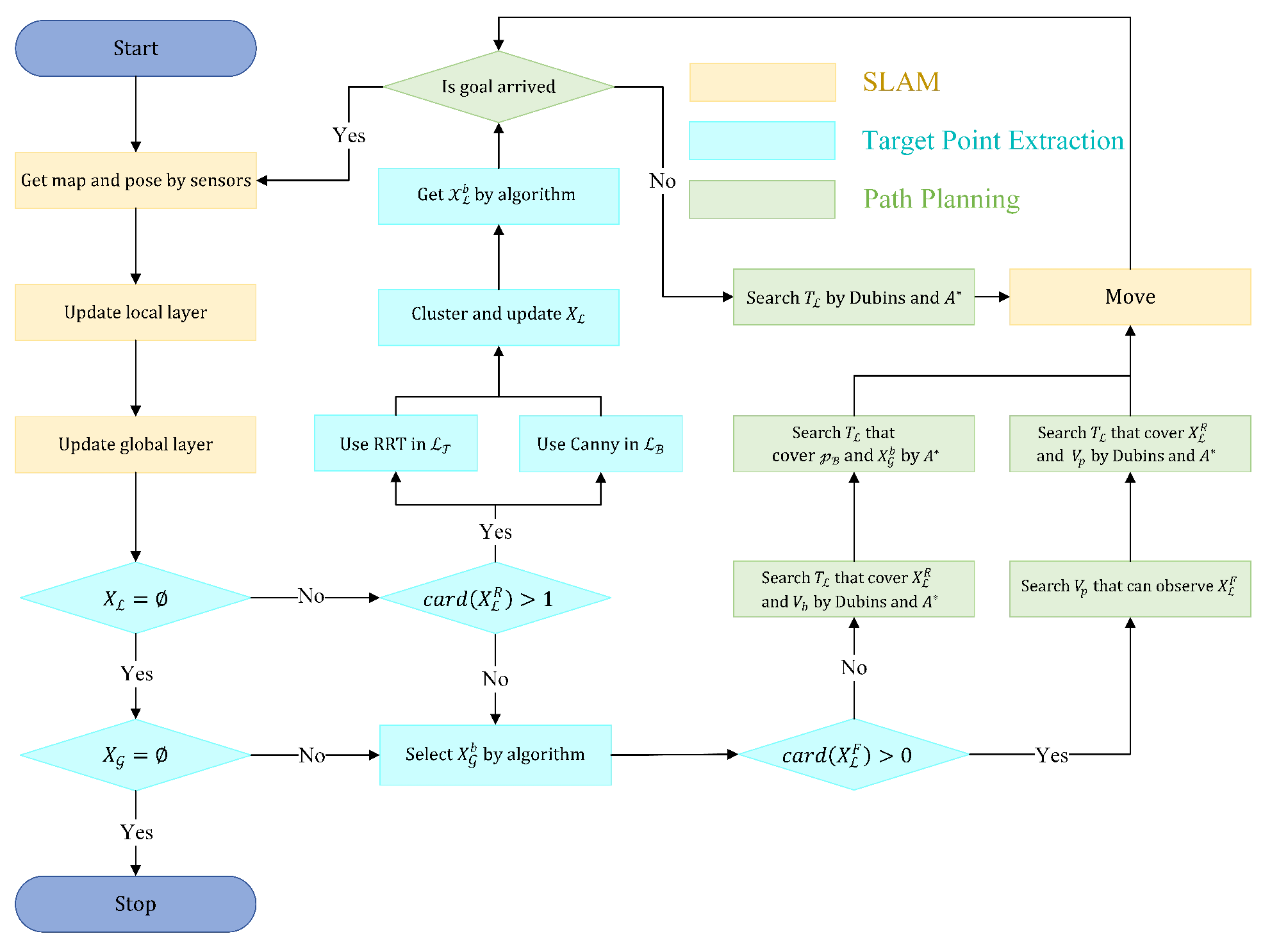
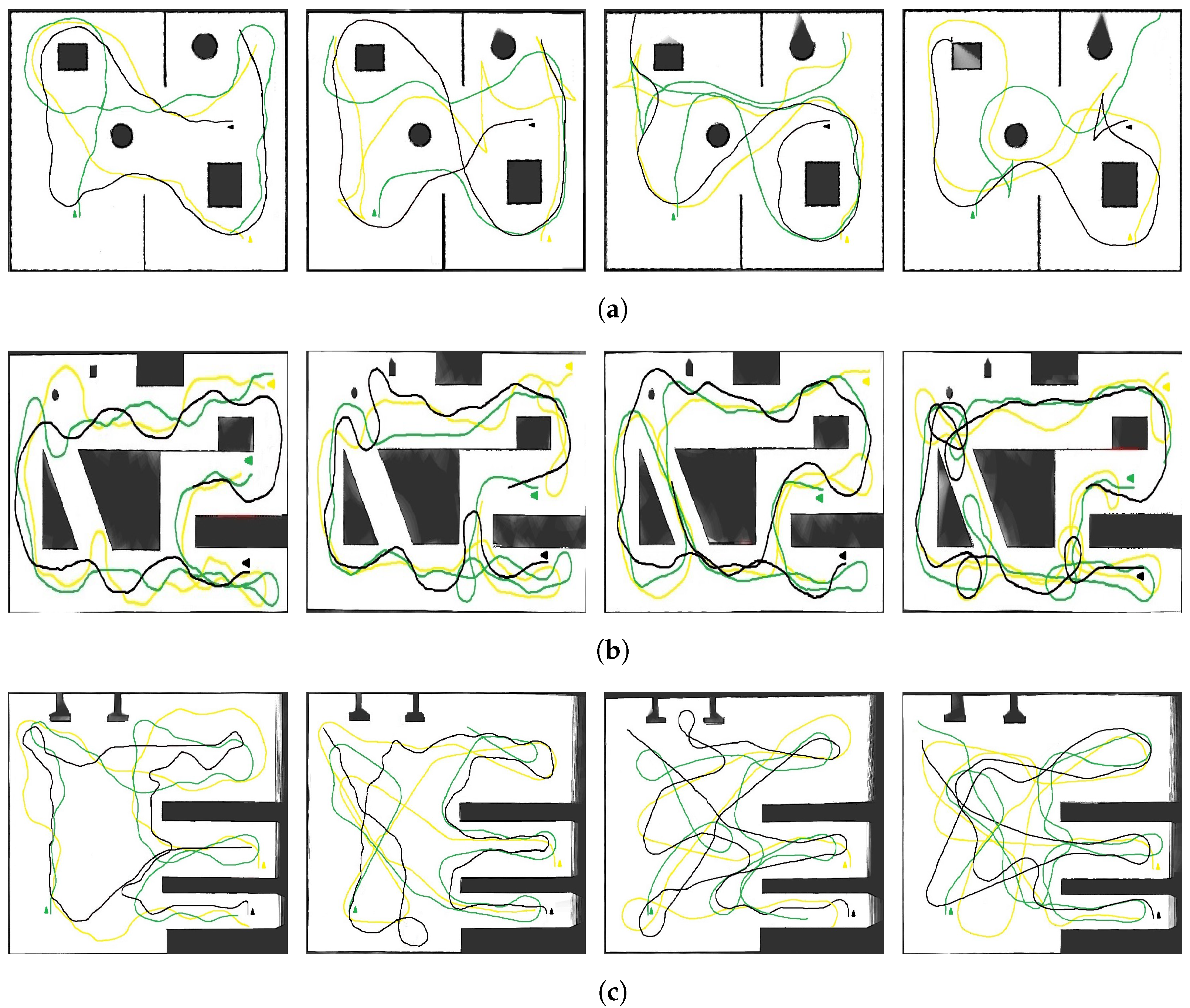
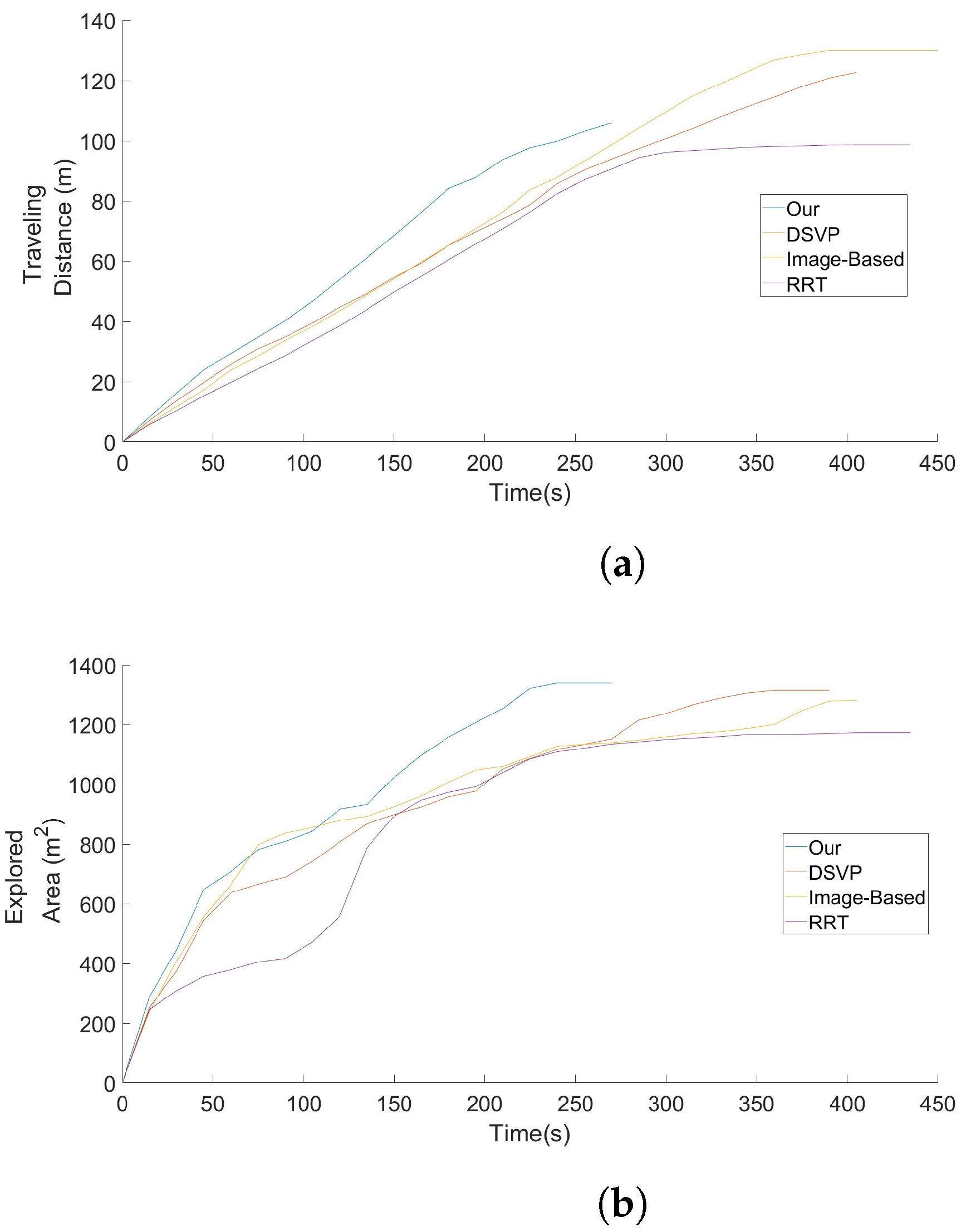
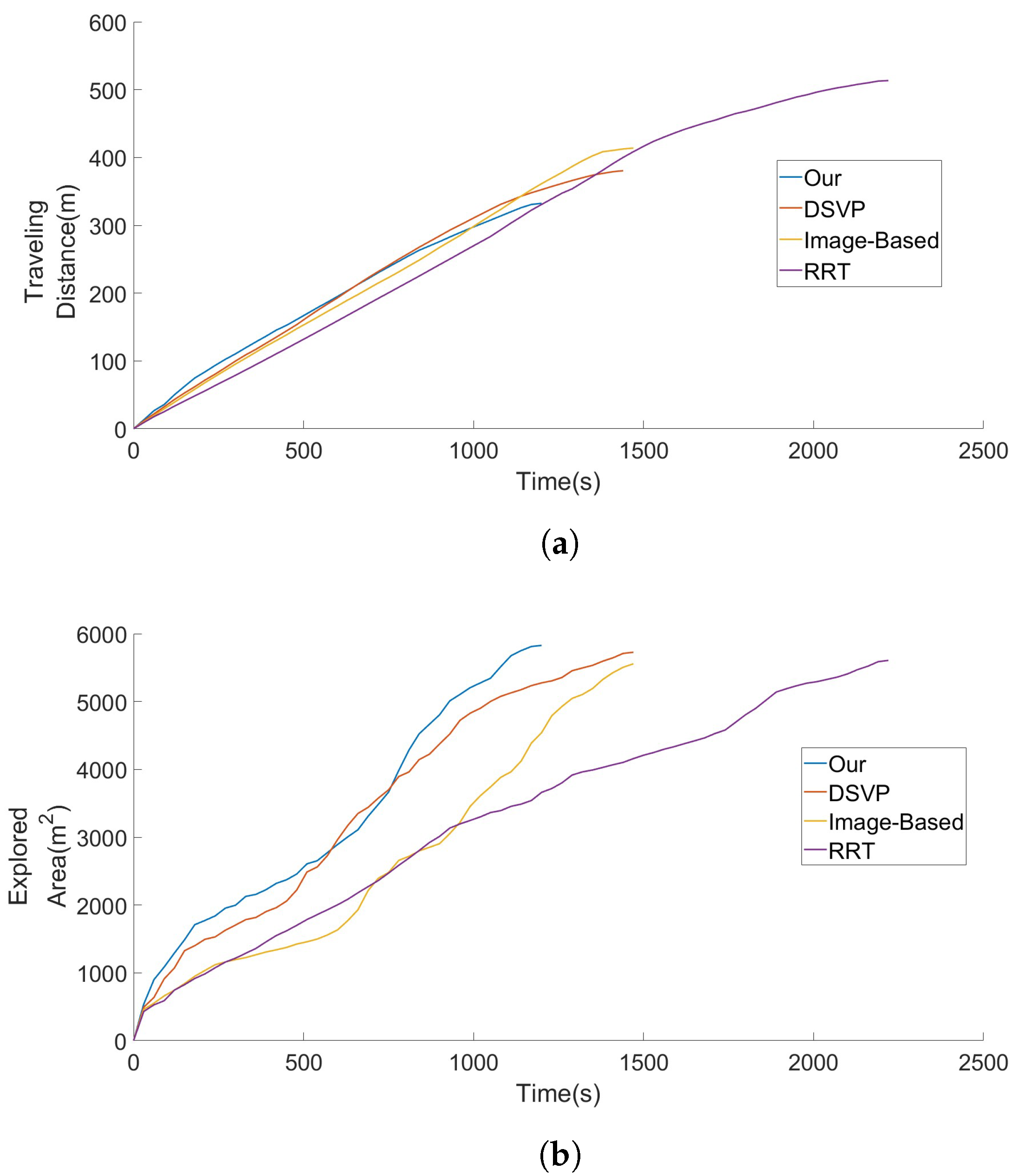
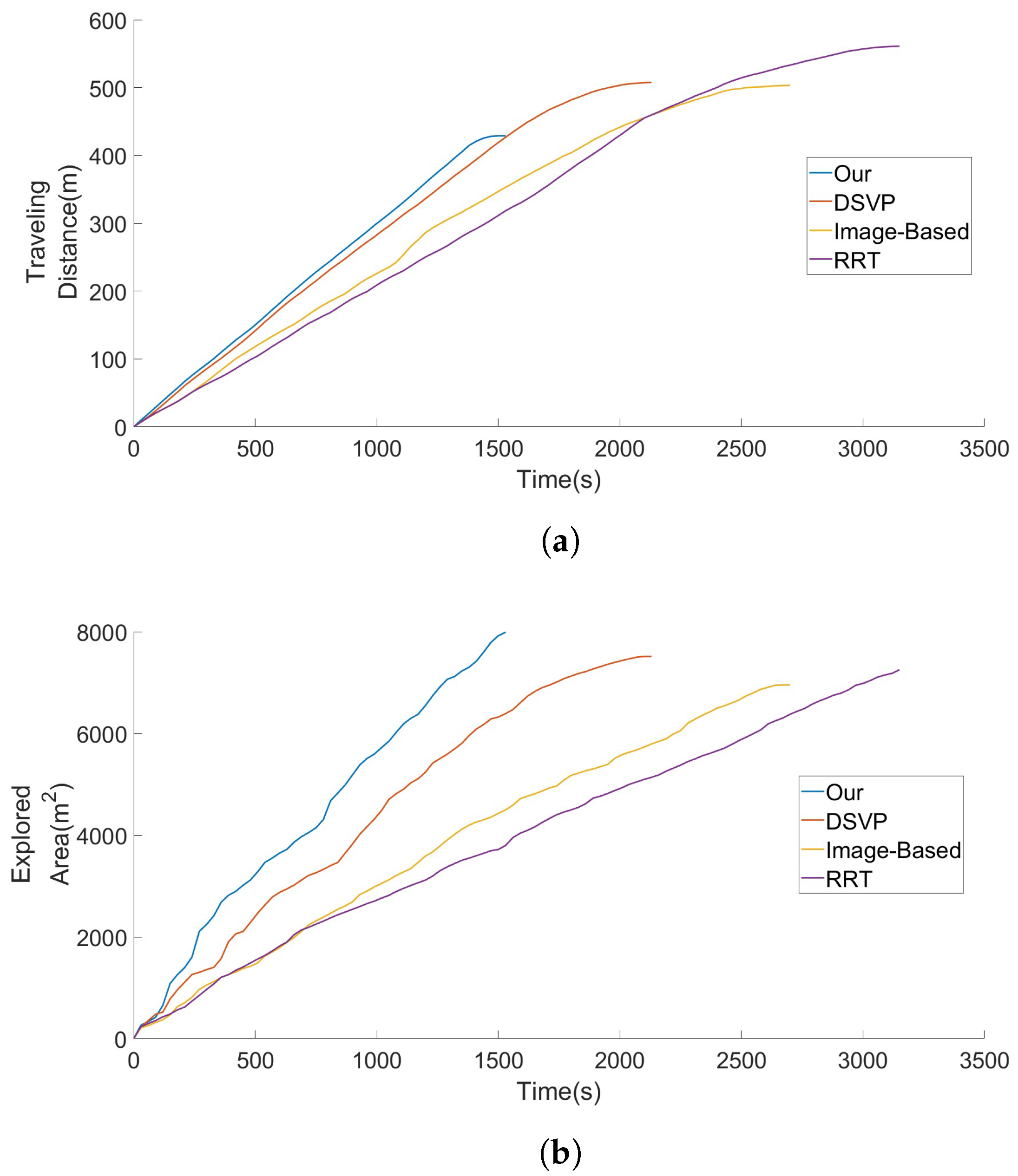
4.1.1. Exploration Phase
The exploration phase is used to extend
. We use dynamic extended RRT and a frontier detection method based on image segmentation to generate observation points around the USV.
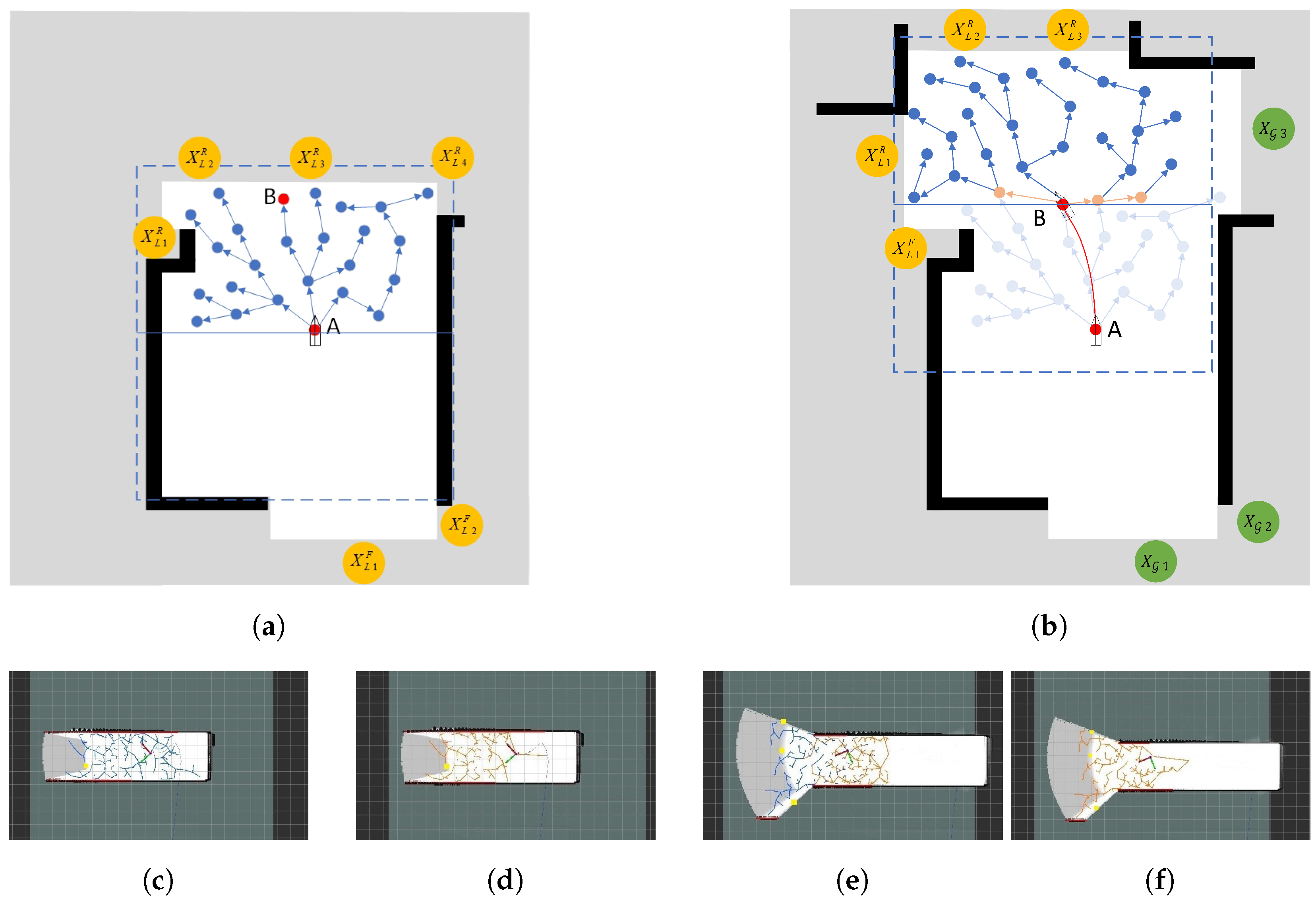
Figure 2a shows the process of the exploration phase, with the USV as the geometric center and the blue dashed region
defined as the local layer. In the process of exploration, RRT and frontier detection methods based on image segmentation are used for partition detection.
Define the upper half of the local layer and create a dynamic random tree with the current position of the USV as the root. The nodes generated by each iteration of the random tree after meeting the boundary are the local observation points in the upper half of the region. RRT is selected for high search space coverage and, in concert with the pruning stage, the growing parts can be retained each time, reducing the calculation cost. Moreover, due to the motion characteristics of the USV, it is not easy to reach the target point behind itself in the local layer. Therefore, RRT is only used to detect the upper half of the region, and priority is given to assigning observation points to the USV first.
Since the growth range of RRT is specified, the growing branches can better go along the direction of the USV, which is conducive to the acquisition of boundary points. Also, because the limited growth range is specified, the possibility of dropping corners is significantly reduced. In the lower part of the local layer , the Canny edge detection method is used, which is consistent with the traditional boundary detection method. Given the grid map and limited exploration area, in this case, it does not take up more memory and has more efficient boundary extraction, and the center of the extracted boundary is selected as the local observation point in the lower half of the region.
In the exploration stage, the relationship of each parameter is described as follows:
In Equation (1),
is defined as the set of local observation points obtained in the exploration phase. The subscripts of
and
, which are obtained by RRT and the edge detection method, represent the order of generating corresponding observation points, and the local observation points are restricted to the local layer. Further,
is the effective field of view of the sensor, and its coverage is smaller than the planning area of the local layer
, while the acquisition process of observation points will be effectively carried out within the scope of
. As a result, the unknown boundary area will be closer to the visual constraint range of
, and the unknown area in
will be acquired more purposefully. Considering the motion characteristics of the USV with limited turning, in the exploration phase, directions are preferentially allocated to the observation points
in the current exploration, while
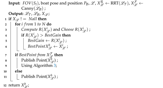
is distributed behind the USV, so priority is not given. All observation points that have not been visited are imported into the global target point set
with delay and lag. Equations (2)–(4) show the gain function used to calculate each local observation point, which is similar to the method used in [
10]. On this basis, the steering gain is added, which is more suitable for the exploration characteristics of the USV.
In Equation (2),
is used to denote all observation points in the local range, and the weight
is used to make the gain
have a similar order of magnitude as the navigation cost
N. Additionally,
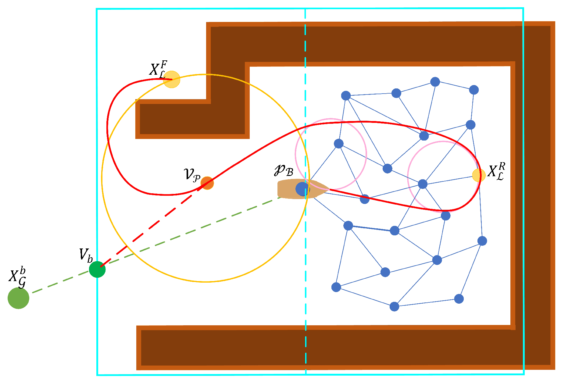
represents the information gain at the observation point, whose size is related to the selection of the sensor, and it is expressed in the form of the unknown area covered. As shown in
Figure 3, the red circular area is defined as the effective field of view of the sensor, and the sum of the yellow and pink areas is defined as the unknown area, which is different from the traditional use of only the yellow area and abandons the small occupied area of the grid. By increasing the information gain, the influence of navigation costs can be reduced, and the USV can go to the local observation point farther away. The information gained from the observation point is expressed as the sum of the yellow and pink areas. Further,
represents the navigation cost of the USV from the current position
to the observation point
. Here, the feasible path generated by obstacle occlusion is not considered but is only represented by Euclidean distance. Also,
represents the steering gain brought by the observation point
, whose specific magnitude is given by Equations (3) and (4). In Equation (3),
represents the radian between the target point and the direction of the USV. Further,
is the steering gain coefficient, and its magnitude is related to
. In Equation (4),
and
represent the steering weight coefficient, which is the order of magnitude used for balance calculation. Here, considering that a large steering angle may have a certain impact on navigation, the selection should meet
to ensure the priority of small angle selection. It can be seen from the selection of
and
that, by the size of
, the steering gain and the steering weight coefficient are calculated, and the USV is encouraged to go to the observation point with a small angle in the current direction; that is, there is a small amplitude of steering during the voyage, which can cover the map more effectively. After obtaining the best observation point, the USV enters the pruning phase when it moves to point B in
Figure 2b after one iteration.
4.1.2. Pruning Phase
The main purpose of pruning is to remove useless RRT nodes from the local layer. The so-called useless nodes are the nodes that are occluded and outside the upper half of the current local layer. As shown in
Figure 2b, firstly, the physical structure of the random tree is updated, and the root is converted from A to B. Secondly, all nodes and branches that are blocked by obstacles and outside the upper part of the current local layer are deleted, such as the light blue nodes and branches in the figure. Finally, the empty node without branches is connected to the current root, B. During the pruning process, new local observation points, namely the orange nodes in the graph, are randomly sampled and added to the local observation point set. Meanwhile, local observation points
that are not in the current local layer are transformed into global observation points and added to the global observation point set
. Note that
does not consist only of the
legacy, but also of
, which is not selected and whose surroundings are not detected during the exploration phase. In the pruning phase, because part of each growth iteration is retained, it will use a smaller amount of computation than the method of regenerating a new local random tree. In addition, the boundary detection algorithm based on image segmentation is collocated. In the process of exploration, the previous phase of
will take part in the composition of the current moment
. This will largely avoid missing unexplored corners due to the random nature of tree growth.
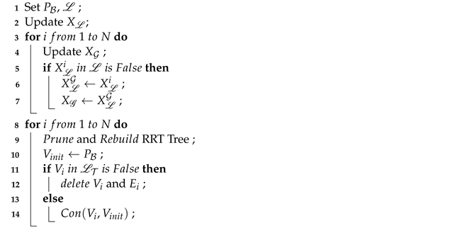
Algorithm 1 defines the detailed process of the pruning phase. The local layer is updated at a constant frequency. At each update, all
values are checked, and the local observation points
, which were dropped into the global layer during the exploration phase, are imported into
. This procedure corresponds to lines 3 through 8 in Algorithm 1. Then,
is transformed into the root node
, and all RRT nodes in
are checked. All nodes
V and branches
E that are not in
are pruned, and the nodes that are not pruned are directly connected to the root node. In terms of code implementation, we designed a
function to connect nodes.
| Algorithm 1: Pruning Phase |
![Jmse 12 01622 i001]() |
4.1.3. Effective Backtracking Phase
Backtracking is inevitable during exploration, but we can avoid invalid backtracking. So-called invalid backtracking refers to the act of repeatedly moving back and forth between a few regional explorations, which greatly reduces exploration efficiency. The backtracking that occurs when the current subarea is fully explored before entering another subarea can be an effective backtrace.
In the exploration process, when there is no unknown boundary information in , that is, , it will change from the local exploration phase to the effective backtracking phase of the global layer. In this phase, the local image observation point , the global layer information , and the global observation point set information are used, and the hierarchical navigation strategy is combined to complete the effective backtracking. Here, , which is not converted to , consists of , left over from the exploration phase. Further, is an incremental map obtained from the beginning of exploration until now, which is mainly used to plan the navigation path of the USV in the backtracking phase. Also, is composed of left over from each iteration. In the iteration process, the global observation point with the nearest distance and the least backtracking cost is selected from as the navigation target point, and a reasonable path is planned through the hierarchical navigation strategy to complete effective backtracking. Here, the selection of the best global observation point follows the generated time order. The time order is determined by marking the time angle index for the global target point . Each backtracking will search from the observation point generated the previous time in . In the backtracking phase, the USV sailed in the area of the known, but it may be gathering information to extend other boundary conditions. The planning of the course may use to cover the unknown boundary, so it needs to update the list of the global observation point . If appears, the exploration work has been completed and the exploration will end.


 ,
, 


