Abstract
A comprehensive analysis was carried out to investigate the driving factors and influencing mechanisms of spatiotemporal variation of sea level at multiple scales in the East China Sea (ECS) via satellite altimetry datasets from 1993 to 2020. Based on the altimetry grid data processed by the local mean decomposition method, the spatiotemporal changes of ECS sea level are analyzed from the multi-scale perspective in terms of multi-year, seasonal, interannual, and multi-modal scales. The results revealed that the ECS regional mean sea level change rate is 3.41 ± 0.58 mm/year over the 28-year period. On the seasonal scale, the regional mean sea level change rates are 3.45 ± 0.66 mm/year, 3.35 ± 0.60 mm/year, 3.39 ± 0.71 mm/year, and 3.57 ± 0.75 mm/year, for the four seasons (i.e., spring, summer, autumn, and winter) respectively. The spatial distribution analysis showed that ECS sea level changes are most pronounced in coastal areas. The northeast sea area of Taiwan and the edge of the East China Sea shelf are important areas of mesoscale eddy activity, which have an important impact on regional sea level change. The ECS seasonal sea level change is mainly affected by monsoons, precipitation, and temperature changes. The spatial distribution analysis indicated that the impact factors, including seawater thermal expansion, monsoons, ENSO, and the Kuroshio Current, dominated the ECS seasonal sea level change. Additionally, the ENSO and Kuroshio Current collectively affect the spatial distribution characteristics. Additionally, the empirical orthogonal function was employed to analyze the three modes of ECS regional sea level change, with the first three modes contributing 26.37%, 12.32%, and 10.47%, respectively. Spatially, the first mode mainly corresponds to ENSO index, whereas the second and third modes are linked to seasonal factors, and exhibit antiphase effects. The analyzed correlations between the ECS sea level change and southern oscillation index (SOI), revealed the consistent spatial characteristics between the regions affected by ENSO and those by the Kuroshio Current.
1. Introduction
The East China Sea (ECS) is a marginal sea bordered by mainland China, Taiwan Island, the Korean Peninsula, Japan’s Kyushu Island, and the Ryukyu islands [1]. The eastern coastal regions of China, where approximately 70% of major cities and over 50% of the population are concentrated, represent the most economically developed areas in the country. However, owing to low terrain and geological factors, these regions are also highly vulnerable to the impacts of sea level rise [2,3,4,5,6,7]. The rising sea level will inevitably bring the challenge of preventing natural disasters, especially for the coastal cities. Investigating the spatiotemporal changes in the ECS sea level holds significant importance for the Yangtze River Delta region, particularly the Shanghai area, in proactively addressing sea level variations [8,9]. Studying the change patterns of the ECS sea level is crucial for coastal cities to develop mid- to long-term disaster prevention and reduction plans and policies to effectively mitigate disaster risks in a timely manner.
Extensive research has investigated both global and regional sea level changes, revealing that sea level variations are influenced by multiple factors. For instance, various elements affecting future sea level changes include ocean thermal expansion, the melting of ice sheets and glaciers, terrestrial water storage, storm surges, tides, waves, El Niño–Southern Oscillation (ENSO), typhoons, atmospheric pressure, ocean circulation, and extreme weather events [10,11,12]. Moreover, there are differences between the observed sea-level changes in different regions and the correlations of these factors at different spatial and temporal scales. Before the advent of satellite altimetry, the analysis of global and regional sea level changes relied primarily on data from tide gauge stations, which offered limited spatial coverage. For example, Jevrejeva et al. [13] proposed a nuanced approach to analyze the permanent sea level (PSMSL) database of global and different regional sea level time series and identified long-term trends, periodic oscillations, and noise components. Given the regional variation characteristics of sea level in the East China Sea, numerous studies have examined these changes across different scales. Specifically, Zhou et al. [14] examined the sea level rise rates in East Asia and along the Chinese coast, highlighting notable variations, particularly a pronounced rise at the mouth of the Yangtze River. Liu et al. [15] delved into the interplay between ECS sea level variations and their responses to ENSO and wind stress. Cheng et al. [16] utilized cyclostationary empirical orthogonal function (CSEOF) analysis to capture regional sea level cycles, shedding light on potential impacts on flood frequency along the Chinese coast. Qu et al. [17] investigated the seasonal sea level cycles surrounding China’s seas, focusing on the key driving factors. Yan et al. [18] explored sea level changes in the East China Sea across different time scales, revealing the influences from the Kuroshio Current and Yangtze River runoff. Recent studies on sea level variations in the East China Sea have analyzed trends in sea level changes and explored the relationships between sea level variations and PDO/ENSO [15,18].
Building upon satellite altimetry data, this chapter employs methodologies including local mean decomposition (LMD), wavelet analysis, the nonstationary sliding correlation analysis method, and empirical orthogonal function (EOF) analysis to investigate the periodic structures and anomalous sea level changes across various time scales in the East China Sea from 1993 to 2020. These sophisticated methods enable a finer-resolution analysis, offering improved precision and the capacity to detect both short-term anomalies and long-term trends. This approach not only enhances our understanding of the mechanisms driving sea level changes but also provides critical insights into potential future scenarios, especially considering the effects of climate change on regional sea levels. The rest of this paper is organized as follows: the materials and methods are briefly presented in Section 2, the results and analysis are presented in Section 3, and the conclusions are presented in Section 4.
2. Study Area, Adopted Datasets, and Methods
2.1. Study Area
The East China Sea, part of the western Pacific marginal seas, lies between mainland China, Kyushu Island, the Ryukyu Islands, and Taiwan Island. Sea level changes in this region significantly affect the nearshore marine ecosystems along the southeastern coast of China [19]. Due to regional geographical factors in the ECS, the Yangtze River estuary carries a large amount of sediment and fresh water to the East China Sea, and together with various factors such as the Kuroshio, ENSO, and sea surface wind stress, it affects the multi-scale variation of sea level.
2.2. Adopted Datasets
The merged gridded sea level anomaly data using multiple satellites, such as ERS-1/2, TOPEX/Poseidon, GFO, Jason-1/2/3, Envisat, and the Sentinel-3A satellite, can be accessed from the website at https://www.aviso.altimetry.fr/en/data/products.html, (accessed on 3 March 2024). which have undergone orbital error corrections between satellite altimeters, along with other error corrections, including atmospheric and tidal corrections. In this work, we study gridded sea level anomaly data from the East China Sea (20–35° N, 120–130° E) region, with a time range from 1993 to 2020 and a spatial resolution of 0.25° × 0.25°. Additionally, the SOI, which measures the El Niño–Southern Oscillation (ENSO), developed by the U.S. Climate Prediction Center (CPC), can be downloaded from the website of https://www.cpc.ncep.noaa.gov/ (accessed on 10 March 2024). Note that normally ENSO events are divided into warm El Niño events and cold La Niña events, which represent the warm and cold phases of the tropical Pacific’s periodic climate pattern.
2.3. Processing Methods
2.3.1. Analysis of ECS Sea Level Change Based on Local Mean Decomposition Method
The global sea level has exhibited an accelerating rising trend for many years [20,21,22]. The primary drivers are attributed to increases in melting ice sheets due to global warming. Indeed, many influence factors including melting glaciers, thermal expansion of seawater, vertical deformation of the Earth’s crust, land subsidence, El Niño–Southern Oscillation (ENSO) events, ocean circulation alterations, etc., have certain contributions to the total sea level change [23,24,25]. Many analysis methods can be used to extract the sea level change signals, with which the local mean decomposition (LMD) method is a novel adaptive signal analysis approach [26]. It decomposes complex time series into diverse frequency components, yielding substantial benefits in processing nonstationary signals [26]. Considering the advantage of LMD for isolating the signals and noise, and separating the time series into long-term trends, period components, and noise terms, we use it to process sea level change series in the ECS to better analyze the characteristics of ECS sea level change.
For the LMD method, the sea level change series can be broken down into different components, such as related trends, periods, and noise, based on a combination of functions, where each function is the product of the envelope signal and the frequency modulation (FM) signal. If the original satellite altimetry grid altimetry data of different longitude–latitudes are specified as , the decomposition results of LMD can be expressed as:
where is the latitude of the satellite altimetry data, is the longitude of the satellite altimetry data, and is the number of PF components decomposed by the sea level data of different longitudes and latitudes. represents the trend component of long-term sea level rise, and represents the different frequency components decomposed by the LMD method from high to low, where the first component may contain irregular terms and change irregularly in the long run. Here, in this study, we remove high-frequency components whose cycles are less than once every three months. The remaining components represent sea level change signals, including long-term trends and other cyclical signals such as annual, semi-annual and seasonal components. Through the improved LMD method, the robustness of multi-scale sea level change data is improved, and the reliability of subsequent analysis is established.
2.3.2. Regional Averaging Method
To calculate the regional mean sea level change from the gridded SLA data, it is important to consider weighting factors for latitude and position and perform regional averaging [27,28,29]. In this study, we use the weighted average method to process the grid data based on satellite altimetry to compute the ECS regional mean sea level change, which is as follows:
where represents the regional average at time points; , represent the geographic location of the data; represents the data value represented at that geographic location, and represents the latitude of that data point.
2.3.3. Wavelet Analysis
Based on the spatiotemporal analysis of sea level change, the wavelet power spectrum can mine more periodic and energy information regarding sea level change to further explore the multi-scale change in sea level. On the basis of the principles of the Fourier transform, the wavelet power spectrum approximates ECS sea level change series via wavelet functions to extract wavelet coefficients and variance integrals [30,31]. We choose the Morlet wavelet function to shift and scale the time series of ECS sea level change, and its wavelet power spectrum can be expressed as:
where represents the time translation factor, represents the scale extension factor, and represents the wavelet transform coefficient.
2.3.4. Nonstationary Sliding Correlation Analysis Method
Considering that sea level change is caused by many impact factors, and the simple analysis of sea level change cannot reflect the specific driving mechanism, the non-stationary sliding correlation analysis method is further used to evaluate the correlations between the two non-stationary geophysical phenomena. The sliding correlation coefficient is a technique for calculating the correlation coefficients within varying time windows [32,33,34]. When investigating the relationship between ECS sea level change and ENSO phenomena, we employ the widely utilized sliding correlation analysis method that is used in climate research. The correlation coefficient between two time series, and , can be expressed as:
where represents the covariance and where and denote the variance. The sliding correlation coefficient can be expressed as:
where ~ represents the sliding value at any window; 一 represents the average. Then, , , and represent the sliding covariance, sliding variance, and difference between the covariance and variance of the entire time period, respectively.
2.3.5. Empirical Orthogonal Function (EOF) Method
EOF analysis is a widely used statistical technique in oceanography and atmospheric sciences. It breaks down the spatiotemporal distribution of variable fields into orthogonal functions, referred to as modes [35]. In order to better understand the spatial and temporal patterns of sea level change, we employed EOF to examine the distribution of various modes. This method is built upon the structural characteristics of variable domains [36]. The primary objective is to approximate and analyze the original field through principal component functions and their linear combinations with eigenvectors. These independent principal components are ordered based on their contribution to total variance. Suppose that there are variables within the definition of an element field, observed times, represented by the corresponding matrix as follows:
The elements are decomposed into a linear combination of spatial and temporal functions, represented by the following expression:
where represents the temporal coefficient, also known as the principal component. denotes the spatial function or the principal component coefficient. The spatial functions are mutually orthogonal.
The specific flowchart of this study is shown in Figure 1.
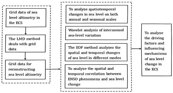
Figure 1.
The flowchart of this study.
3. Results and Analysis
3.1. Annual Variations of ECS Sea Level Change
The LMD method decomposes satellite altimetry data into high-frequency, low-frequency, and trend components based on local characteristic scales within the data. By analyzing local mean values, it identifies instantaneous frequencies and amplitudes, enabling the differentiation of short-term fluctuations like tides, storm surges, internal waves, and mesoscale eddies, as well as seasonal variations and long-term sea level trends. The method’s adaptability allows for the extraction of components with clear physical significance, surpassing traditional methods in handling complex, nonlinear, and non-stationary signals. Considering that sea level changes often include both low-frequency signals of long-term variations and high-frequency signals of short-term fluctuations, the LMD method effectively filters out high-frequency components from the SLA data, as demonstrated in the East China Sea grid dataset from January 1993 to December 2020, referring to Section 2.3.1.
After removing the high-frequency components, the ECS sea level change signal is obtained by reconstructing the altimetry grid data. The average annual SLA over 27 years in ECS is shown in Figure 2. Figure 3 shows the spatial distribution of the linear trend in the mean annual sea level change in the ECS.
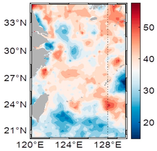
Figure 2.
The ECS average SLA (mm) for the period 1993 to 2020.
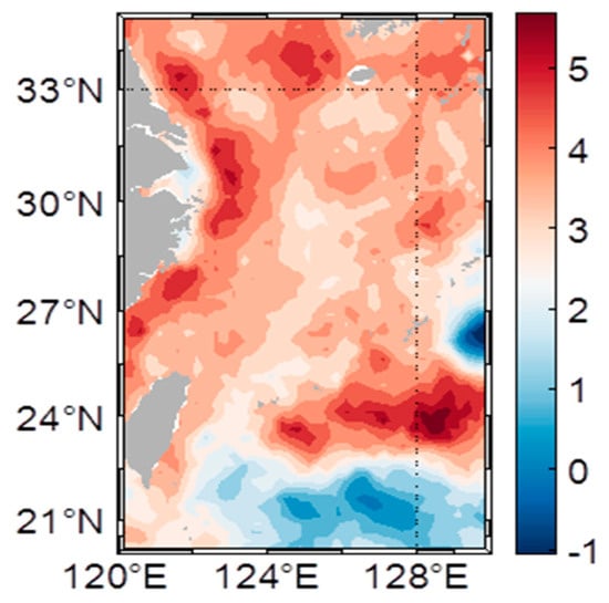
Figure 3.
The ECS sea level change rates (mm/year) for the period 1993 to 2020.
The ECS sea level changes exhibit multiscale circulation characteristics, with the Shanghai plane circulation influenced by the runoff of the Yangtze River and the Kuroshio Tide on an annual scale [18]. As depicted in Figure 2, the annual average ECS sea level is 37.95 mm. Owing to the impact of the East Asian monsoon, the spatial distribution of multiyear mean ECS sea level is higher in the North China Sea and lower in the south. Shanghai, located in the low-lying Yangtze River Delta, is particularly vulnerable to rising sea levels from the East China Sea. This exposes the city to increased flooding, storm surges, and saltwater intrusion, endangering its infrastructure and water resources. Other cities like Ningbo, Wenzhou, Zhoushan, Fuzhou, and Xiamen are also at risk, though Shanghai’s dense population and economic role make its situation more critical. Population density and heavy construction lead to coastal subsidence, and worsening sea level-rise effects. In cities like Shanghai, this increases the threat of flooding and infrastructure harm. Figure 3 shows that 56.83% of the annual average change rate exceeds the mean, with most coastal areas in the East China Sea experiencing notable rise in sea level, particularly near the mouth of the Yangtze River Delta. The East China Sea is generally high in the west and low in the east, with a greater rising rate at the mouth of the Yangtze River. The northeastern waters of Taiwan and the East China Sea shelf edge are key areas for mesoscale eddy activity along the Kuroshio Current. Due to the instability of the Kuroshio boundary current, baroclinic effects, and the complex underwater topography, mesoscale eddies frequently form in these regions. These eddies play a significant role in influencing local ocean dynamics and sea level changes. Specifically, at the East China Sea shelf edge, the influence of Kuroshio branch currents intensifies the formation and activity of these eddies. Additionally, these phenomena influence regional ocean circulation and, by affecting sea surface temperatures and atmospheric circulation patterns, interact with long-term climate phenomena such as Pacific Decadal Oscillation (PDO), which typically spans over ten years. This interaction further impacts the area’s ocean climate and sea level changes [15,18].
To analyze the ECS sea level change as a whole for the study period, the regional mean sea level change series is computed based on Equation (2) of the regional averaging method. As shown in Figure 4, the ECS regional mean sea level change rate is 3.41 ± 0.58 mm/year for the period from 1993 to 2020, with an acceleration rate of −0.04 mm/year2, as calculated via the least squares fitting method. Note that the corresponding uncertainty represents the least-squares fitting error. When using the LMD (local mean decomposition) method, there is a possibility that certain high-frequency components may be filtered out, potentially causing a slight underestimation of acceleration value. However, the impact on the overall analysis is mild.
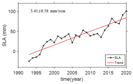
Figure 4.
ECS regional mean sea level change from 1993 to 2020. (The black line indicates the annual average SLA, while the red line shows the annual rate of increase from 1993 to 2020).
3.2. Seasonal Variations of ECS Sea Level Change
In Section 3.1, the annual variations of ECS sea level change were analyzed in detail. However, affected by a combination of factors such as seawater thermal expansion and seasonal monsoons [37], seasonal change characteristics notably exist in regional sea level change; therefore, we will further analyze the ECS sea level change from the perspective of seasonal patterns. Note that four seasons are divided into spring (March to May), summer (June to August), autumn (September to November), and winter (December to February). The average gridded ECS sea level changes for the four seasons are computed, which are shown in Figure 5. From Figure 5, we can find that the multiyear average reaches its peak value in autumn and its lowest value in spring, with coastal areas experiencing higher sea level anomalies in summer and autumn than the other two seasons. Considering that the East China Sea is a marginal sea with the depths along the coast mostly less than 200 m, the coastal sea level change is significantly influenced by sea surface temperatures. The offshore area of East China Sea is notably influenced by the Kuroshio Current, with relatively smaller seasonal variations than those of coastal regions [38].
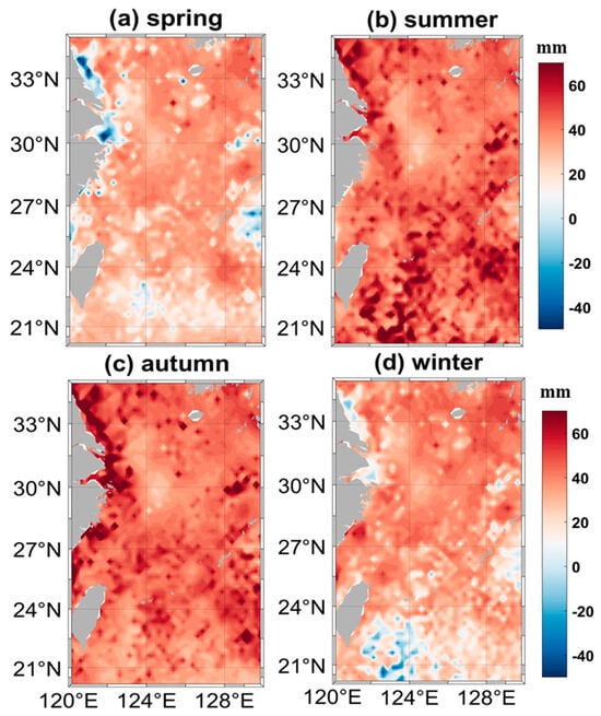
Figure 5.
The spatial distributions of ECS averaged SLA for four seasons, for the period from January 1993 to December 2020 (mm). (Average sea level distributions for (a) spring, (b) summer, (c) autumn, and (d) winter, with red indicating higher values and blue indicating lower values, allowing direct comparison across all seasons).
Analysis of the seasonal spatial distribution reveals that wave patterns vary significantly with changes in monsoon wind direction. The summer and winter monsoons have a pronounced impact on wave behavior, making spring and autumn transitional periods where dominant wave patterns are less distinct. During the summer, the ECS is primarily affected by the southward monsoon. High temperatures and moderate rainfall, combined with low wind speeds, contribute to lower sea levels in the coastal regions of the northwest. As the season transitions to autumn, the sea experiences southerly winds with sustained low wind speeds, moderate temperatures, and decreased rainfall, leading to a rise in sea levels along the coast. In winter, the ECS is dominated by the northeast monsoon, bringing cooler temperatures, reduced rainfall, prolonged wind activity, and the year’s highest wind speeds, resulting in a low sea level center southeast of Taiwan Island. The Yangtze River, the largest river in East Asia, flows through ten provinces and cities (including autonomous regions) before emptying into the ECS. At the mouth of the Yangtze River, where it flows into the East China Sea, the sediment carried by freshwater begins to increase in volume during January. This sediment transport reaches its peak in March, and then starts to decrease, hitting its lowest point in August [39]. During the summer, the Yangtze River experiences its rainy season, leading to a considerable increase in runoff into the sea. This surge in freshwater discharge causes noticeable shifts in coastal sea levels, as captured by the spatial distribution of satellite altimetry data, which clearly reflects these seasonal variations. In contrast, during winter, the runoff gradually decreases, along with a reduction in freshwater flux. These changes are similarly evident in the satellite altimetry measurements, indicating lower coastal sea levels in areas affected by the diminished river inflow.
Seasonal spatial distribution analysis indicates that sea level in the East China Sea peaks in autumn, driven by the combined effects of summer southerly winds and the Yangtze River’s freshwater flux. Additionally, the Yangtze River estuary is prone to storm surges during summer and autumn, contributing to rapid short-term sea level fluctuations in coastal areas.
The linear-trend spatial distributions of ECS sea level change for the four seasons are presented in Figure 6. For the rates which exceed the ECS, regional mean sea level change rates account for 93.99%, 91.46%, 91.88%, and 93.71% of total area for the four seasons, respectively. From Figure 6, it is significant to find that the sea level change exhibits a decreasing trend in the southeastern ECS region (Kuroshio main axis basin) and an increasing trend in the northwestern ECS region. The areas with lower change rates are primarily concentrated in the southeast of Taiwan Island. This spatial differentiation, shaped by the Kuroshio Current, reflects our method’s capability to precisely capture regional sea level trends, showcasing its effectiveness in analyzing complex oceanographic patterns.
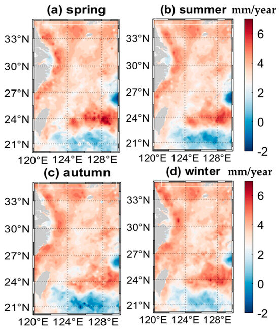
Figure 6.
The linear-trend spatial distributions of ECS sea level change for four seasons over the period from 1993 to 2020. (Spatial distribution of the annual average sea level rise rate for (a) spring, (b) summer, (c) autumn, and (d) winter, with red indicating higher values and blue indicating lower values, allowing direct comparison of sea level distribution across all seasons).
An analysis of ECS regional mean sea level changes for the four seasons (spring, summer, autumn, winter) is performed for the period from 1993 to 2020, which is shown in Figure 7. The estimated rates of ECS seasonal sea level changes for the four seasons are 3.45 ± 0.66 mm/year, 3.35 ± 0.60 mm/year, 3.39 ± 0.71 mm/year, and 3.57 ± 0.75 mm/year, respectively, indicating that the sea level rise rates in spring and winter are larger than those in summer and autumn.
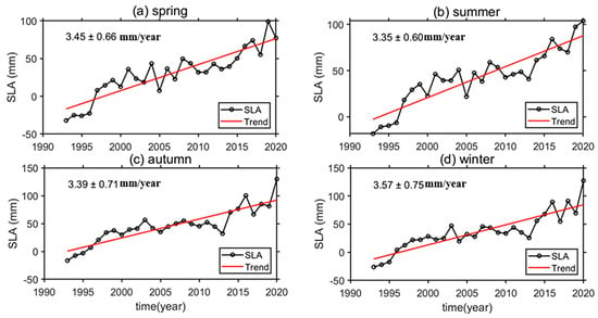
Figure 7.
Four seasonal ECS regional mean sea level changes for 1993 to 2020.
The ECS regional mean sea level change rate exhibited the lowest increase in summer and the highest in winter. As shown in Figure 7a,b, the fluctuations in ECS sea level change are more significant in spring and summer than those in autumn and winter, which is attributed to the combined impact of seasonal factors including the temperature, rainfall, and monsoons [40,41]. It is clearly to find that the ECS sea level change peaked to 129.85 mm in autumn 2020 (Figure 7c). The estimated ECS regional sea level change rates and acceleration, mean change and increase amplitude for the four seasons over the period from 1993 to 2020, are presented in Table 1. Based on our analysis of the spatial and temporal distribution and calculated data regarding sea level variations, distinct seasonal patterns emerged in the East China Sea from 1993 to 2020. In spring, the rate of sea level rise slows down, indicating a transitional period during which the climate warms and oceanic systems adjust. During summer, although the pace of sea level rise is relatively slower, significant changes are still observed, driven by the influence of monsoons and the thermal expansion of seawater. In autumn, the sea level stabilizes, with minimal fluctuations, which aligns with the relatively steady meteorological and oceanic conditions during this season. Winter, however, shows the most pronounced variability, with the sea level rising at the fastest rate and exhibiting the highest levels of fluctuation and acceleration throughout the year, primarily due to frequent cold air activity and changes in ocean circulation during this period.

Table 1.
The estimated ECS regional sea level change rates and acceleration, mean change, and increasing amplitude for the four seasons over the period from 1993 to 2020.
3.3. Modal Analysis of ECS Regional Mean Sea Level Change
Long-term sea level variations are mainly driven by low-frequency components, which represent more sustained and gradual trends. These components are essential for gaining insight into the fundamental patterns of sea level rise, as they are less influenced by transient fluctuations and uncertainties. Consequently, in order to analyze the long-term ECS sea level change more accurately on the interannual time scale, the high-frequency component of short-term sea level change containing uncertainty is removed from the ECS sea level change series, and the low-frequency component of long-term sea level change is reconstructed.
The wavelet power spectrum was subsequently used to analyze the time series, with those results displayed in Figure 8. As shown in Figure 8b, the ECS regional mean sea level changes exhibited notably periodic characteristics within a 95% confidence interval from 2000 to 2008 and from 2013 to 2019. The predominant periodic components include 1 year, 2 years, and 3 years, where the 2- and 3-year periodic components have higher energy values in the wavelet power spectrum. The 1-year cycle corresponds to seasonal factors like monsoons and shifts in atmospheric pressure, leading to predictable sea level changes annually. The 2-year cycle is tied to interannual phenomena such as the El Niño–Southern Oscillation (ENSO), which affects sea levels by altering ocean–atmosphere interactions. The 3-year cycle relates to more complex oceanic processes, including fluctuations in the Kuroshio Current’s trajectory and intensity, impacting regional ocean circulation and sea level patterns.
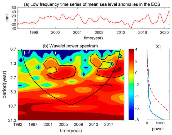
Figure 8.
Wavelet Analysis of ECS regional mean sea level change. (Figure 8a shows the low-frequency components of the sea level time series. Figure 8b displays the wavelet energy spectrum, where red indicates higher energy and blue lower energy; the circled area passes the significance test. Figure 8c illustrates the energy values from the spectrum).
Indeed, the ECS regional mean sea level changes are influenced by various factors, necessitating a method that can effectively isolate these influences. EOF analysis is particularly useful as it breaks down sea level data into dominant variability modes. This approach helps identify key patterns and provides a clearer understanding of the factors driving long-term trends. Through empirical orthogonal function (EOF) analysis, three modes and their corresponding time coefficients were obtained, as shown in Figure 9. The spatial contributions of the first three modes are 26.37%, 12.32%, and 10.47%, respectively. The variance accounted for by the EOF modes beyond the first three is likely associated with more localized or higher-frequency variations, including mesoscale eddies or transient atmospheric effects. While these factors contribute to sea level fluctuations, their impact on long-term trends is less significant compared to the dominant modes. The spatial distributions of the first three modes indicate that the first and second modes are essentially complementary in space. The second mode exhibits similarities with the spatial distribution of seasonal variations and displays distinct seasonal variation characteristics. The correlation coefficients between the time coefficients corresponding to the three EOF modes and the SOI are 0.68, 0.035, and 0.004, respectively, indicating a strong correlation between the first mode and ENSO phenomenon. The first mode corresponds to the ENSO mode, and analysis of the time coefficient reveals a certain correlation with decadal sea level change. Moreover, the seawater depths northeast of Taiwan Island exceed 1000 m, making this area less susceptible to the thermal expansion effects of seawater induced by the ENSO phenomenon, with greater impacts observed southeast of Taiwan Island. The coastal regions experience a reduced impact primarily due to freshwater influx and anthropogenic factors, as the intensified circulation of water masses obscures interannual variability. Additionally, the influence of mesoscale eddies further diminishes the significance of the impact northeast of Taiwan [42]. In summary, the analysis verifies that the first EOF mode is closely linked to ENSO, emphasizing its substantial impact on decadal sea level variations in the East China Sea. Additionally, it shows that the deep waters northeast of Taiwan are less influenced by ENSO-induced thermal expansion, while the effects are more significant southeast of Taiwan. This underscores the critical role of spatial variability in comprehending regional sea level responses to global climate factors.
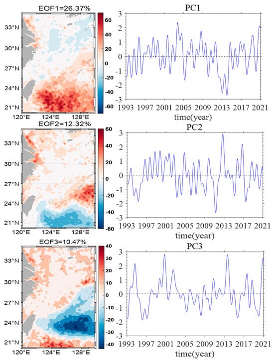
Figure 9.
EOF Analysis of SLA Variations in the ECS.
A correlation analysis method was subsequently employed to examine the relationship between the EOF analysis results and the ENSO phenomenon, with the obtained results depicted in Figure 10a. An analysis of the spatial distribution of the correlation coefficients between the SOI and ECS regional mean sea level change was subsequently conducted, as illustrated in Figure 10b. The results revealed that ECS sea level changes were significantly influenced by ENSO; notably, pronounced impacts were observed in the northern and southern regions of Taiwan Island, where most correlation coefficients exceeded 0.3. Furthermore, coastal cities in the southern part of the ECS are more susceptible to the influence of ENSO, with the majority of correlation coefficients being positive. Areas near Xiamen and Lianyungang are particularly susceptible to the effects of ENSO, with most correlation coefficients exceeding 0.1. The seasonal variation patterns and spatial distributions of ENSO and sea level changes typically exhibit contrasting tendencies, suggesting an antiphase relationship between the influences of ENSO and seasonal factors on sea level changes. The seasonal variations in sea level are relatively consistent at middle and high latitudes, with greater variability observed at low latitudes.
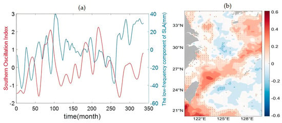
Further analysis was conducted on the spatial correlation between ECS sea level change and the SOI across the entire ECS region. The percentage of positive correlations that exceeded the significance test was 40.75%, whereas the percentage of negative correlations was 1.62%. The spatial distribution clearly indicates the impact of ENSO on the sea level anomalies in the ECS, which is particularly evident in regions where the Kuroshio Current flows, highlighting a significant correlation. This phenomenon illustrates that ENSO impacts sea level changes, with the affected regions being spatially correlated with the direction and magnitude of the main axis flow of the Kuroshio. The interaction between ENSO and the Kuroshio Current mainly impacts the Kuroshio’s main axis, where the current is most intense. ENSO-induced shifts in atmospheric and oceanic dynamics directly affect this region, modifying the Kuroshio’s strength, path, and heat transport. This leads to intricate sea level variations, with El Niño typically diminishing the Kuroshio and reducing sea levels, while La Niña enhances it, raising sea levels. These dynamics highlight the pivotal role of the Kuroshio’s main axis in regional sea level trends driven by ENSO [43].
4. Conclusions
In this study, we comprehensively analyzed the ECS sea level changes by employing advanced methodologies including local mean decomposition (LMD), wavelet analysis, the nonstationary sliding correlation analysis method, and empirical orthogonal function (EOF) analysis, which provide the following valuable insights. The regional sea level variations in the East China Sea are influenced by a combination of factors, such as freshwater flux, sea surface wind stress, ENSO, the Kuroshio Current, tidal effects, storm surges, sedimentation, and human activities. These factors contribute to notable uncertainties, periodicity, and long-term trends in ECS sea level. The findings of this study indicate a regional mean sea level rise rate of 3.41 ± 0.58 mm/year, with an average sea level value of approximately 37.92 mm.
The seasonal sea level changes exhibited distinct trends, with higher rates of increase observed in winter and summer than the other two seasons. Specifically, the sea level change rates in winter and summer are 3.45 ± 0.66 mm/year and 3.57 ± 0.75 mm/year, respectively, whereas in spring and autumn, they are 3.35 ± 0.60 mm/year and 3.39 ± 0.71 mm/year, respectively. This highlights the significance of seasonal factors in ECS sea level dynamics. Spatial distribution analysis revealed that the factors, including seawater thermal expansion, monsoons, ENSO, and the Kuroshio Current, dominated the ECS seasonal sea level change. The results show that the seasonal sea level changes are most significant along the southeastern coast of Taiwan, with correlation coefficients mostly exceeding 0.3, and notably impacting the seas near Xiamen and Lianyungang, where most correlation coefficients just exceed 0.1.
Empirical orthogonal function (EOF) analysis revealed the first three modes for ECS sea level change, accounting for 26.37%, 12.32%, and 10.47% of the total variance, respectively. The first mode is closely related to ENSO, whereas the subsequent modes are closely related to seasonal factors, exhibiting antiphase impacts on sea level changes. Correlation analysis between the ECS sea level changes and the southern oscillation index (SOI) reveals that the impact of ENSO on the East China Sea aligns mainly with the intrusion area of the Kuroshio Current. Most correlation coefficients exceed 0.1, particularly in the seas near Xiamen and Lianyungang. These findings indicate that our research is highly sensitive to the driving mechanisms and potential causes of ECS sea level changes, effectively capturing the temporal and spatial complexities involved. Future research could integrate additional data sources, such as GRACE and other types of remote sensing data, to further explore the driving mechanisms and comprehensive impacts on sea level changes in the East China Sea.
Author Contributions
Conceptualization, F.W. and L.X.; methodology, F.W. and L.X.; validation, F.W. and Y.J.; resources, F.W.; writing—original draft, F.W. and L.X.; writing—review and editing, Y.J.; visualization, L.X.; supervision, Y.J.; and project administration, Y.J. All authors have read and agreed to the published version of the manuscript.
Funding
This work is sponsored by the Natural Science Foundation of China (42374017).
Institutional Review Board Statement
Not applicable.
Informed Consent Statement
Not applicable.
Data Availability Statement
The raw data supporting the conclusions of this article will be made available by the authors without undue reservation.
Conflicts of Interest
The authors declare that the research was conducted in the absence of any commercial or financial relationships that could be construed as potential conflicts of interest.
References
- Qu, Y.; Jevrejeva, S.; Jackson, L.; Moore, J.C. Coastal Sea level rise around the China Seas. Glob. Planet. Chang. 2019, 172, 454–463. [Google Scholar] [CrossRef]
- Nicholls, R.; Cazenave, A. Sea-level rise and its impact on coastal zones. Science 2010, 328, 1517–1520. [Google Scholar] [CrossRef]
- IPCC. Climate Change 2013. The Physical Science Basis: Working Group I Contribution to the Fifth Assessment Report of the Intergovernmental Panel on Climate Change; Cambridge University Press: Cambridge, UK, 2014. [Google Scholar]
- IPCC. Climate Change 2021: The Physical Science Basis. Contribution of Working Group I to the Sixth Assessment Report of the Intergovernmental Panel on Climate Change; Masson-Delmotte, V., Zhai, P., Pirani, A., Connors, S.L., Péan, C., Berger, S., Caud, N., Chen, Y., Goldfarb, L., Gomis, M.I., Eds.; Cambridge University Press: Cambridge, UK; New York, NY, USA, 2021. [Google Scholar] [CrossRef]
- Siegert, M.; Alley, R.; Rignot, E.; Englander, J.; Corell, R. Twenty-first century sea-level rise could exceed IPCC projections for strong-warming futures. One Earth 2020, 3, 691–703. [Google Scholar] [CrossRef]
- Xu, Y.; Lin, M.; Zheng, Q.; Ye, X.; Li, J.; Zhu, B. A study of long-term sea level variability in the East China Sea. Acta Oceanol. Sin. 2015, 34, 109–117. [Google Scholar] [CrossRef]
- Hu, Z.; Yang, S.; Wu, R. Long-term climate variations in China and global warming signals. J. Geophys. Res. Atmos. 2003, 108, D19. [Google Scholar] [CrossRef]
- Wang, J.; Gao, W.; Xu, S.; Yu, L. Evaluation of the combined risk of sea level rise, land subsidence, and storm surges on the coastal areas of Shanghai, China. Clim. Chang. 2012, 115, 537–558. [Google Scholar] [CrossRef]
- Chen, X.; Zong, Y. Major impacts of sea-level rise on agriculture in the Yangtze delta area around Shanghai. Appl. Geogr. 1999, 19, 69–84. [Google Scholar] [CrossRef]
- Church, J.; Godfrey, J.; Jackett, D.; McDougall, T.J. A model of sea level rise caused by ocean thermal expansion. J. Clim. 1991, 4, 438–456. [Google Scholar] [CrossRef]
- Pokhrel, Y.; Hanasaki, N.; Yeh, P.; Yamada, T.J.; Kanae, S.; Oki, T. Model estimates of sea-level change due to anthropogenic impacts on terrestrial water storage. Nat. Geosci. 2012, 5, 389–392. [Google Scholar] [CrossRef]
- Zuo, J.; He, Q.; Chen, C.; Chen, M.X.; Xu, Q. Sea level variability in East China Sea and its response to ENSO. Water Sci. Eng. 2012, 5, 164–174. [Google Scholar]
- Jevrejeva, S.; Grinsted, A.; Moore, J.; Holgate, S. Nonlinear trends and multiyear cycles in sea level records. J. Geophys. Res. Ocean. 2006, 111, C9. [Google Scholar] [CrossRef]
- Zhou, X.; Zheng, J.; Doong, D.; Demirbilek, Z. Sea level rise along the East Asia and Chinese coasts and its role on the morphodynamic response of the Yangtze River Estuary. Ocean Eng. 2013, 71, 40–50. [Google Scholar] [CrossRef]
- Liu, X.; Liu, Y.; Guo, L.; Rong, Z.; Gu, Y.; Liu, Y. Interannual changes of sea level in the two regions of East China Sea and different responses to ENSO. Glob. Planet. Chang. 2010, 72, 215–226. [Google Scholar] [CrossRef]
- Cheng, Y.; Plag, H.; Hamlington, B.; Xu, Q.; He, Y. Regional sea level variability in the Bohai sea, Yellow sea, and East China Sea. Cont. Shelf Res. 2015, 111, 95–107. [Google Scholar] [CrossRef]
- Qu, Y.; Jevrejeva, S.; Williams, J.; Moore, J.C. Drivers for seasonal variability in sea level around the China seas. Glob. Planet. Chang. 2022, 213, 103819. [Google Scholar] [CrossRef]
- Yan, M.; Zuo, J.; Du, L.; Li, L.; Li, P.L. Sea level variation/change and steric contributions in the East China Sea. In Proceedings of the ISOPE International Ocean and Polar Engineering Conference, Lisbon, Portugal, 1–6 July 2007; Volume ISOPE-I-07-129. [Google Scholar]
- Wang, G.; Kang, J.; Yan, G.; Han, G.; Han, Q. Spatio-temporal variability., sea level in the East China Sea. J. Coast. Res. 2015, 73, 40–47. [Google Scholar] [CrossRef]
- Church, J.; Clark, P.; Cazenave, A.; Gregory, J.M.; Jevrejeva, S.; Levermann, A.; Merrifield, M.A.; Milne, G.A.; Nerem, R.S.; Nunn, P.D.; et al. Sea Level Change; PM Cambridge University Press: Cambridge, UK, 2013. [Google Scholar]
- Cazenave, A.; Llovel, W. Contemporary sea level rise. Annu. Rev. Mar. Sci. 2010, 2, 145–173. [Google Scholar] [CrossRef]
- Carson, M.; Köhl, A.; Stammer, D.; Slangen, A.B.A.; Katsman, C.A.; van de Wal, R.S.W.; Church, J.; White, N. Coastal sea level changes, observed and projected during the 20th and 21st century. Clim. Chang. 2016, 134, 269–281. [Google Scholar] [CrossRef]
- Cazenave, A.; Henry, O.; Munier, S.; Delcroix, T.; Gordon, A.L.; Meyssignac, B.; Llovel, W.; Palanisamy, H.; Becker, M. Estimating ENSO influence on the global mean sea level, 1993–2010. Mar. Geod. 2012, 35 (Suppl. S1), 82–97. [Google Scholar] [CrossRef]
- Shepherd, A.; Wingham, D. Recent sea-level contributions of the Antarctic and Greenland ice sheets. Science 2007, 315, 1529–1532. [Google Scholar] [CrossRef]
- Zemp, M.; Huss, M.; Thibert, E.; Eckert, N.; McNabb, R.W.; Huber, J.; Barandun, M.; Machguth, H.; Nussbaumer, S.U.; Gärtner-Roer, I.; et al. Global glacier mass changes and their contributions to sea-level rise from 1961 to 2016. Nature 2019, 568, 382–386. [Google Scholar] [CrossRef]
- Smith, J. The local mean decomposition and its application to EEG perception data. J. R. Soc. Interface 2005, 2, 443–454. [Google Scholar] [CrossRef] [PubMed]
- Cazenave, A.; Dominh, K.; Gennero, M.; Ferret, B. Global mean sea level changes observed by Topex-Poseidon and ERS-1. Phys. Chem. Earth 1998, 23, 1069–1075. [Google Scholar] [CrossRef]
- Dong, X.; Huang, C. Monitoring Global Mean Sea Level Variation with TOPEX/Poseidon Altimetry. J. Geod. Geoinf. Sci. 2000, 3, 266–272. [Google Scholar]
- Nerem, R.S. Measuring Global Mean Sea Level Variations Using TOPEX/Poseidon Altimeter Data. J. Geophys. Res. 1995, 100, 25135–25151. [Google Scholar] [CrossRef]
- Shafieloo, A.; Souradeep, T.; Manimaran, P.; Panigrahi, P.K.; Rangarajan, R. Features in the primordial spectrum from WMAP: A wavelet analysis. Phys. Rev. D 2007, 75, 123502. [Google Scholar] [CrossRef]
- Torrence, C.; Compo, G. A practical guide to wavelet analysis. Bull. Am. Meteorol. Soc. 1998, 79, 61–78. [Google Scholar] [CrossRef]
- Rodríguez-Fonseca, B.; Suárez-Moreno, R.; Ayarzagüena, B.; López-Parages, J.; Gómara, I.; Villamayor, J.; Mohino, E.; Losada, T.; Castaño-Tierno, A. A review of ENSO influence on the North Atlantic. A non-stationary signal. Signal. Atmos. 2016, 7, 87. [Google Scholar]
- He, S.; Wang, H. Oscillating relationship between the East Asian winter monsoon and ENSO. J. Clim. 2013, 26, 9819–9838. [Google Scholar] [CrossRef]
- Geng, X. Decadal and Subseasonal Variations of ENSO Impacts on the East Asian Winter Climate and Their Mechanisms. D. Nanjing University of Information Science and Technology: Nanjing, China, 2018. [Google Scholar]
- Hannachi, A.; Jolliffe, I.; Stephenson, D. Empirical orthogonal functions and related techniques in atmospheric science: A review. Int. J. Climatol. A J. R. Meteorol. Soc. 2007, 27, 1119–1152. [Google Scholar] [CrossRef]
- Weare, B.; Nasstrom, J. Examples of extended empirical orthogonal function analyses. Mon. Weather Rev. 1982, 110, 481–485. [Google Scholar] [CrossRef]
- Lombard, A.; Cazenave, A.; DoMinh, K.; Cabanes, C.; Nerem, R.S. Thermosteric sea level rise for the past 50 years; comparison with tide gauges and inference on water mass contribution. Glob. Planet. Chang. 2005, 4, 303–312. [Google Scholar] [CrossRef]
- Kawabe, M. Inter-annual Variations of Sea Level at the Nansei Islands and Volume Transport of the Kuroshio Due to Wind Changes. J. Oceanogr. 2001, 2, 189–205. [Google Scholar] [CrossRef]
- Chang, L.; Tang, H.; Yi, S.; Sun, W. The trend and seasonal change of sediment in the East China Sea detected by GRACE. Geophys. Res. Lett. 2019, 46, 1250–1258. [Google Scholar] [CrossRef]
- Bowen, M.M. Wind-driven and steric fluctuations of sea surface height in the southwest Pacific. Geophys. Res. Lett. 2006, 33, 14. [Google Scholar] [CrossRef]
- Chen, J.; Shum, C.K.; Wilson, C.R.; Chambers, D.P.; Tapley, B.D. Seasonal sea level change from Topex/Poseidon observation and thermal contribution. J. Geod. 2000, 73, 638–647. [Google Scholar] [CrossRef]
- Zhang, S.; Du, L.; Wang, H.; Jiang, H. Regional sea level variation on interannual timescale in the East China Sea. Int. J. Geosci. 2014, 5, 1405–1414. [Google Scholar] [CrossRef]
- Jo, S.H.; Moon, J.H.; Kim, T.; Song, Y.T.; Cha, H. Interannual modulation of kuroshio in the East China Sea over the past three decades. Front. Mar. Sci. 2022, 9, 909349. [Google Scholar] [CrossRef]
Disclaimer/Publisher’s Note: The statements, opinions and data contained in all publications are solely those of the individual author(s) and contributor(s) and not of MDPI and/or the editor(s). MDPI and/or the editor(s) disclaim responsibility for any injury to people or property resulting from any ideas, methods, instructions or products referred to in the content. |
© 2024 by the authors. Licensee MDPI, Basel, Switzerland. This article is an open access article distributed under the terms and conditions of the Creative Commons Attribution (CC BY) license (https://creativecommons.org/licenses/by/4.0/).