Development of a Spectrum-Based Scheme for Simulating Fine-Grained Sediment Transport in Estuaries

Abstract

Fine-grained cohesive sediments in estuaries play a critical role in sediment transport and biogeochemical cycles in estuaries. Due to the convergence of marine saltwater and freshwater runoff, combined with periodic tidal cycles, fine-grained sediments exhibit intricate flocculation processes that are challenging to simulate. A size-resolved flocculation module using a bin-based scheme aids in modeling these processes but is hindered by high computational costs. In this study, we develop a new spectrum-based scheme based on the spectral shape of floc size distribution from the original bin-based scheme to expedite modeling execution. This new scheme is implemented in the Stony Brook Parallel Ocean Model (sbPOM) and applied to simulate fine-grained sediment transport in the Hudson River estuary. The effectiveness of this spectrum-based scheme is assessed by comparing its simulations with observations and results from the original bin-based scheme. The findings indicate that the new scheme can simulate the evolution of suspended sediment concentration well at a specific point by comparisons with in-situ observations. Specifically, the results of the 50 paired experiments show an average percentage difference of 1.86% and an average speedup ratio of 4.51 times compared to the original bin-based scheme. In summary, the new spectrum-based scheme offers significant acceleration benefits for the size-resolved flocculation module and has the potential for widespread application in simulating fine-grained sediments in estuaries.

1. Introduction

Estuaries are a key route for sediment to be transported from rivers to adjacent seas [1,2]. Sediments, which may be contaminated, are often retained in estuaries and hence can significantly affect environments and socio-economic activities, such as water clarity, pollution, eutrophication, navigation channel maintenance, dredge spoil disposal, and so on [3,4,5]. Within this context, fine-grained cohesive sediments are particularly critical. Due to their relatively small particle size, resulting in a large relative surface area per unit volume, flocs formed through flocculation are a porous and loosely structured entity capable of entrapping a large amount of organic matter as well as heavy metals, which is believed to have a substantial impact on environment [6,7,8].

Fine-grained sediments (silt and clay particles) in estuaries experience complex processes like transport, flocculation, settling, deposition, consolidation, and resuspension [9]. Due to the variable hydrological conditions in estuaries, sediment dynamics in these waters are more active than in the upstream rivers [10]. Specifically, the geographical location of estuaries is unique, situated at the confluence of the ocean and terrestrial runoff. The water properties on either side exhibit significant differences in salinity, temperature, current velocity, and sediment content. Interaction and exchange between these waters at the estuaries lead to various phenomena in fine-grained sediments, such as estuary turbidity maximum [11,12], suspended sediment front [13,14], fluid mud [15,16], and so on.

Researchers employ various methods to study fine-grained sediments, including field investigations, laboratory experiments, and numerical simulations [17,18]. In the development of fine-grained sediment transport models [19,20], the simulation of flocculation is difficult but valuable [21,22,23]. One notable method is employing the size-resolved flocculation module, which is favored for its ability to explicitly simulate the aggregation and breakup of fine-grained sediments under highly variable conditions [24,25,26,27].

In the size-resolved flocculation module, fine-grained sediments are categorized into a series of bins based on particle size. Generally, tens of bins are used, and the higher the bin number, the more accurate the simulation [24,28]. Each bin has its own characteristics, including radius, settling velocity, suspended sediment concentration (SSC), etc. Interactions occur across different size bins, with smaller particles aggregating into larger ones, and larger particles breaking up into smaller ones. Although this type of module can effectively simulate flocculation processes of fine-grained sediments, a notable drawback is the considerable computational time cost [29,30], including flocculation and advection, due to numerous variables induced by tens of bins [22,24,26,28].

Noticeably, when flocs reach equilibrium in the water column, they tend to distribute like a spectral shape, confirmed by some observations [31,32,33]. This occurs because small (large) flocs have a higher (lower) probability of aggregation (breakup) than breakup (aggregation), making the distribution of particle size skew towards a successive prominent spectrum around the median floc size, resembling a spectral shape [24,26,33].

Based on this distribution form, a new spectrum-based scheme is developed to improve the efficiency of advection in the size-resolved flocculation module. The runtime and simulation bias between the original bin-based scheme [24,34] and the newly developed spectrum-based scheme are compared. The two different schemes are then implemented in a three-dimensional ocean general circulation model, and simulation in the Hudson River estuary is conducted. The results are compared with in-situ observations, and the runtime and bias of the two schemes are compared as well.

The rest of the paper is organized as follows: A size-resolved flocculation module with a newly developed spectrum-based scheme is presented in Section 2. Section 3 describes the setup and validation of the numerical simulation in the Hudson River estuary. The simulation results with the bin-based scheme and the spectrum-based scheme are given in Section 4, with detailed comparisons of runtime and bias. A summary and discussion of the spectrum-based scheme are provided in Section 5.

2. Methods

2.1. A Size-Resolved Flocculation Module

Based on the Smoluchowski framework [35], size-resolved flocculation modules are widely used to simulate sediment transport in estuaries [9,24,27,34]. This model considers mass conservation for particles in different floc size bins. For each specific bin, the basic mass conservation equation is:

$$\frac{\partial n(m,t)}{\partial t}=\frac{1}{2}{\int }_{m_0}^{m}n(m_1,t)K(m_1,m_2)n(m_2,t)d{m}_2$$

$$-{\int }_{m_0}^{\mathrm{\infty }}n(m,t)K(m,m_3)n(m_3,t)d{m}_3$$

$$+{\int }_{m_0}^{\mathrm{\infty }}Q\left(m,m_4\right)P\left(m_4\right)n\left(m_4,t\right)d{m}_4-n\left(m,t\right)P\left(m\right)$$

(1)

where the change rate of the particle number density $n(m,t)$ is a function of mass $m$ and time $t$, the first two terms on the right-hand side denote the aggregation processes, and the last two terms on the right-hand side denote the breakup processes.

The first term on the right, $\frac{1}{2}{\int }_{m_0}^{m}n(m_1,t)K(m_1,m_2)n(m_2,t)d{m}_2$, describes the generation rate of mass $m$ by the aggregation of two smaller particles $m_1,m_2(m=m_1+m_2)$, where $m_0$ is the mass of the first bin and $K$ is the aggregation kernel. The second term, ${\int }_{m_0}^{\mathrm{\infty }}n(m,t)K(m,m_3)n(m_3,t)d{m}_3$, describes the loss rate of mass $m$ when the particles aggregate with other particle mass $m_3$ and then become a bigger one. The third term, ${\int }_{m_0}^{\mathrm{\infty }}Q(m,m_4)P\left(m_4\right)n(m_4,t)d{m}_4$, describes the generation rate of mass $m$ when a bigger particle of mass $m_4$ breaks into mass $m$ and mass $m_4-m$, where $Q$ and $P$ are the functions related to the breakup. The fourth term, $n(m,t)P\left(m\right)$, denotes the loss rate when the particle mass $m$ breaks.

To efficiently solve the mass conservation equation, we convert the grid of integrable variables from the Cartesian coordinate to the logarithmic coordinate [24,34]. The converted relationship between the two coordinates is $y=\mathrm{l}\mathrm{n}r$, with the differential relationship between $dy$ and $dm$ being $g\left(y,t\right)dy=mn\left(m,t\right)dm$. Then, the mass conservation equation in the logarithmic coordinate is derived:

$$\frac{\partial g_{k,floc}}{\partial t}=\frac{1}{2}{\int }_{y_0}^y\frac{m^2}{m_c^2{m}^{\prime }}g\left(y_c,t\right)K\left(y_c,y^{\prime }\right)g\left(y^{\prime },t\right)d{y}^{\prime }$$

$$-{\int }_{y_0}^{\infty }\frac{1}{m^{\prime }}g\left(y_k,t\right)K\left(y_k,y^{\prime }\right)g\left(y^{\prime },t\right)d{y}^{\prime }$$

$$+{\int }_{y_0}^{\infty }\frac{m}{m^{\prime }}Q\left(y_k,y^{\prime }\right)P\left(y^{\prime }\right)g\left(y^{\prime },t\right)d{y}^{\prime }-g\left(y_k,t\right)P\left(y_k\right)$$

(2)

where $g_{k,floc}$ is the suspended sediment concentration (SSC) density function for the flocculation process of bin $k$ at time $t$. Logarithmic mass grid $y_k=ln{r}_k$ with the radius $r_k$ of flocs for bin $k$ and $y_0=ln{r}_0$ is the first mass grid [28].

For the flocs of mass $m$, the first two terms on the right-hand side of Equation (2) indicate the aggregation progress: The first term denotes the increase in bin $k$ due to the aggregation of flocs of mass $m_c$ (the corresponding radius is $y_c$) and $m^{\prime }$($y^{\prime }$), satisfying $m=m_c+m^{\prime }$; the second term denotes the decrease due to aggregation with flocs of other size bins. The last two terms on the right-hand side of Equation (2) indicate the breakup progress: The third term denotes the increase in the breakup of larger flocs; and the fourth term denotes the decrease due to breakup into smaller flocs.

In Equation (2), $K$ is the aggregation kernel, ${K=\alpha ·(K}_{ts}+K_{ds})$ [36,37], describing the rate of floc collision, with $\alpha$as the particle stickiness. The turbulence shear kernel [38] is $K_{ts}=4/3·G{(r_i+r_j)}^3$, with $r_i$ and $r_j$being the radius of flocs for bin $i$ and $j$, respectively. The differential settling kernel [39] is$K_{ds}=\pi \cdot {\left(r_i+r_j\right)}^2\cdot \left|w_{i,settle}-w_{j,settle}\right|$, with $w_{i,settle}$ and $w_{j,settle}$ being the settling velocity of flocs for bins $i$ and $j$, respectively. Meanwhile, the settling velocity is calculated by the formula $w_{i,settle}=0.0002{\left(2r_i\right)}^{1.54}$, where $r_i$ is the floc radius in $\mu m$and $w_{i,settle}$ in $mm/s$ [39]. Note that the effect of Brownian motion is negligible in estuaries and coastal regions [40,41].

$P$is the breakup kernel, calculated by $P\left(y_k\right)=E\sqrt{\mu /F_y}{G}^{1.5}\left(2r_k\right){\left(\right(r_k-r_0)/r_0)}^{3-n_f}$ [42], where $E$ is a tunable parameter, $\mu$ is the dynamic viscosity, $F_y\approx {10}^{-10}Pa$ is the estimated yield strength, $n_f$ is the fractal dimension, and $Q$is the breakup pattern for size variations of daughter flocs. The binary breakup is used after the breakup process, defined as $Q=2,ifm=m^{\prime }/2;Q=0,\mathrm{o}\mathrm{t}\mathrm{h}\mathrm{e}\mathrm{r}\mathrm{w}\mathrm{i}\mathrm{s}\mathrm{e}$ [43].

Considering the aggregation kernel $K$ for fine-grained sediments, the smaller the particle size, the easier they aggregate. Conversely, for breakup kernel $P$, the larger the particle size, the easier they break. In other words, for small particles, aggregation dominates over breakup, while for large particles, breakup dominates over aggregation, leading to a spectral-shaped distribution [24,26,28,33].

For bin $k$, the SSC density function $g_k$ satisfies the governing equation for sediment transport:

$$\frac{\partial g_k}{\partial t}+\frac{\partial u{g}_k}{\partial t}+\frac{\partial v{g}_k}{\partial t}+\frac{\partial (w-w_{k,settle})g_k}{\partial z}=\frac{\partial g_{k,floc}}{\partial t}+\frac{\partial }{\partial z}\left({\epsilon }_{sz}\frac{\partial g_k}{\partial z}\right)$$

(3)

where $u$ and $v$ are the horizontal velocity, $w$ is the vertical velocity, and ${\epsilon }_{sz}$ is the vertical eddy diffusivity.

Equation (3) describes the temporal change in the SSC density function. On the left-hand side, the second and third terms represent the horizontal advection, and the fourth term represents the difference between vertical advection and vertical settling. On the right-hand side, the first term represents the change in SSC due to flocculation (i.e., Equation (2)); the second term represents vertical diffusion.

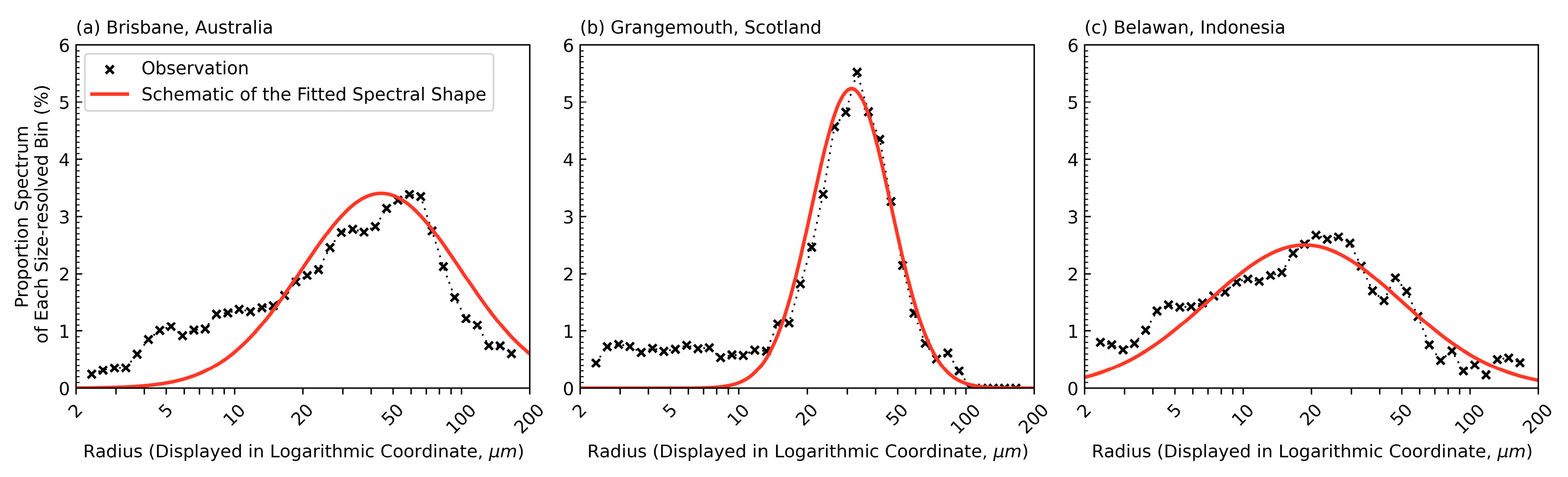
2.2. Spectrum-Based Scheme

In this study, we propose applying a normal distribution in the logarithmic coordinate to fit the floc distribution of SSC along the bin size (detailed derivation is in Appendix B). $f\left(y_k\right)$ is the fitted SSC of bin $k$:

$$f\left(y_k\right)=\frac{\widehat{m}}{\widehat{\sigma }\sqrt{2\pi }}·\mathit{exp}\left(-\frac{{\left(y_k-\widehat{\mu }\right)}^2}{2\widehat{{\sigma }^2}}\right)$$

(4)

where $\widehat{m},\widehat{\mu },$and $\widehat{\sigma }$ are the fitting parameters for the spectral shape.

The estimated mass parameter $\widehat{m}\left(t\right)$ at time $t$ for Equation (4) follows:

$$\widehat{m}\left(t\right)={\sum }_{k=1}^{nbin}{g}_k\left(t\right)\cdot \mathsf{\Delta }{y}_k$$

(5)

where $g_k\left(t\right)$ is the SSC density of bin $k\left(k=\mathrm{1,2},...,nbin\right),nbin$is the bin number, and $\mathsf{\Delta }{y}_k=\ln {(r}_{k+1}/r_k)$ is the bin interval width in the logarithmic coordinate.

The estimated median floc size parameter $\widehat{\mu }\left(t\right)$ at time $t$ for Equation (4) satisfies the first-moment estimation [44,45] for the spectrum, given by:

$$\widehat{\mu }\left(t\right)=\frac{\sum _{k=1}^{nbin}{y}_k\cdot g_k\left(t\right)}{\sum _{k=1}^{nbin}{g}_k\left(t\right)}$$

(6)

The estimated standard deviation parameter $\widehat{\sigma }\left(t\right)$ at time $t$ for Equation (4) satisfies the second-moment estimation for the spectrum, given by:

$$\widehat{{\sigma }^2}\left(t\right)=\frac{\sum _{i=1}^{nbin}{y}_k^2\cdot g_k\left(t\right)}{\sum _{i=1}^{nbin}{g}_k\left(t\right)}-{\left(\frac{\sum _{i=1}^{nbin}{y}_k\cdot g_k\left(t\right)}{\sum _{i=1}^{nbin}{g}_k\left(t\right)}\right)}^2$$

(7)

To illustrate this spectrum-based scheme more visually, we applied it to fit spectral shapes in the Brisbane estuary, Grangemouth estuary, and Belawan estuary [32]. The schematic diagrams are shown in Figure 1, showing that the floc size distribution can generally fit a normal distribution in the logarithmic coordinate.

Then, the number estimation $\widehat{N}\left(t\right)$ is obtained from the mass $\widehat{m}\left(t\right)$ and median floc size $\widehat{\mu }\left(t\right)$, and $\widehat{N}\left(t\right)=\widehat{m}\left(t\right)/(4/3·\pi {\left(\exp \widehat{\mu }\left(t\right)\right)}^3)$ under the spherical assumption. Since mass and number are conserved during advection, the original advection for tens of bins is converted to advection for $\widehat{m}\left(t\right)$ and $\widehat{N}\left(t\right)$. Considering the distribution is continuously changing and the variation is small at the given time $t$, the standard deviation parameter $\widehat{\sigma }\left(t\right)$ becomes fixed at this moment. In summary, discrete bins are encoded into the spectral shape by fitting parameters, followed by advection for the spectral shape, and finally decoded into discrete bins for the next calculation.

A threshold function for error control is employed since floc distributions are not always well fitted by a normal distribution. The absolute percentage error (APE) between the new spectrum-based scheme and the original bin-based scheme is defined as:

$$APE=\frac{{\sum }_{k=1}^{nbin}\left|g_k-f\left(y_k\right)\right|}{{\sum }_{k=1}^{nbin}\left|g_k\right|}$$

(8)

If the APE is smaller than a certain given value (e.g., 10%), the spectrum-based scheme takes effect for advection, replacing the original bin-based scheme. Otherwise, the spectrum-based scheme is prohibited.

3. Numerical Experiments of the Hudson River Estuary

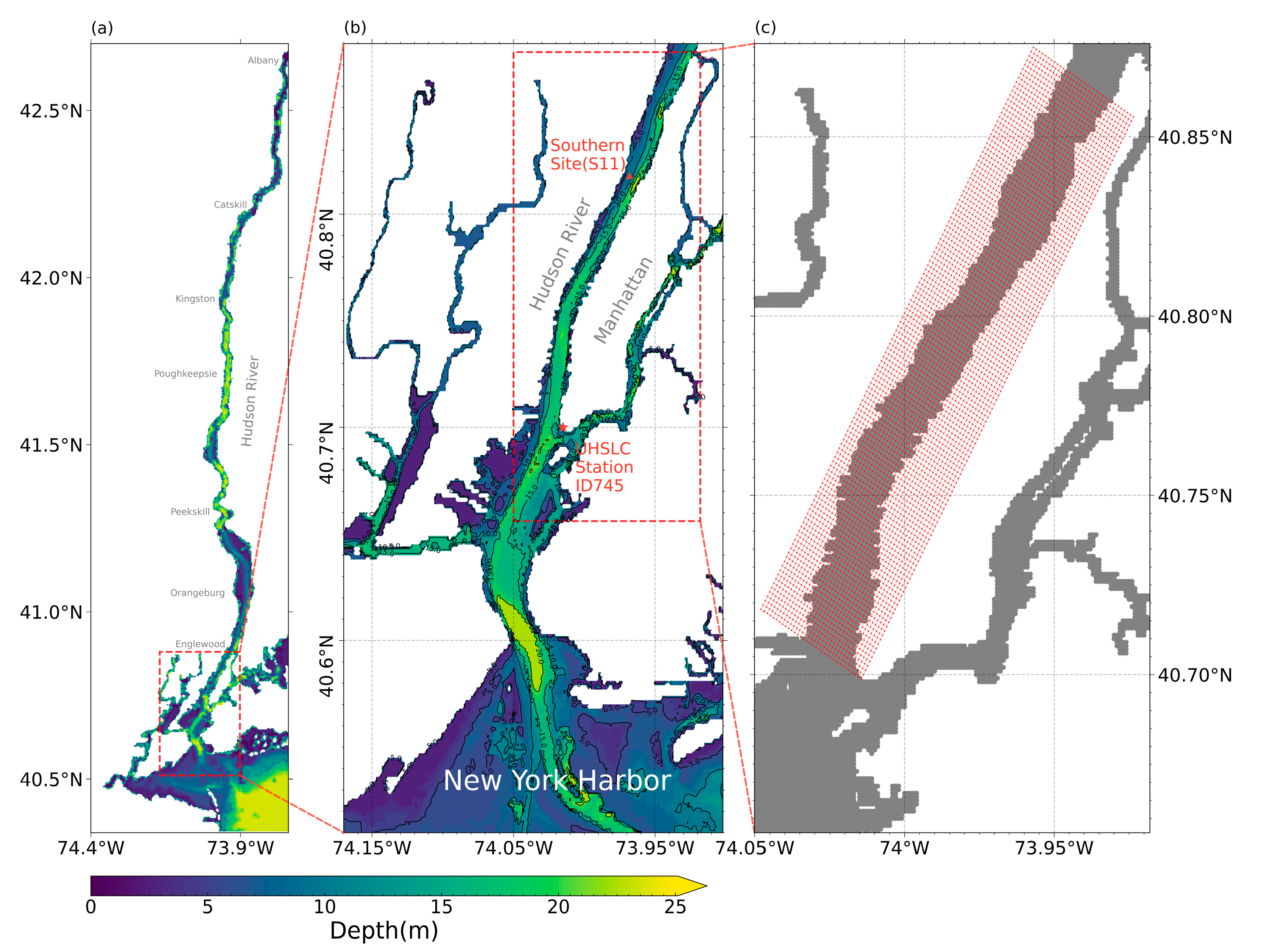
To test the newly developed spectrum-based scheme, we apply the scheme in the Stony Brook Parallel Ocean Model (sbPOM) [46] and conduct numerical experiments for fine-grained sediment transport in the Hudson River estuary.

The Hudson River originates in the Adirondack Mountains and flows southward through the Hudson Valley to the New York Harbor, eventually draining into the Atlantic Ocean. The Hudson River estuary (Figure 2b) is a dynamic and ecologically rich area, where freshwater from the Hudson River mixes with saltwater from the Atlantic Ocean, and plays a crucial role in the geography and ecosystem of New York [47,48,49]. Among extensive programs related to the Hudson River, an observation program implemented by Traykovski [33], including hydrodynamics and sediments, helps to validate the numerical simulation.

3.1. Model Setup

The sbPOM is developed from the Princeton Ocean Model (POM) [50], coupled with biogeochemical modules [51,52] and sediment modules [34,53]. The model is in a terrain-following sigma coordinate in the vertical direction with curvilinear orthogonal coordinates in the horizontal direction and an embedded second-moment turbulence closure sub-model for vertical mixing coefficients [54]. Moreover, it has many operational applications, as demonstrated by its use in simulating oceanographic conditions in the Aegean Sea for oil-drift predictions [55] and in revealing the relationship between sea surface temperature cooling and cross-type typhoon paths [56]. The sbPOM is a relatively simple parallelization to maintain the POM legacy and provide developers with a familiar code that can be easily used or modified.

Figure 2 shows the model domain, from 73.92° W to 74.05° W and from 40.70° N to 40.88° N. The horizontal grid number is 32 × 128. The water depth varies from about 1 m to 21.89 m, with six sigma layers. $\sigma =0$ represents the water surface, $\sigma =-1$represents the riverbed, and the interval between them is evenly divided into six stretched terrain-following sigma layers in the vertical dimension. The topologic map is obtained by combining the navigational chart of the Hudson River and New York Harbor from the National Oceanic and Atmospheric Administration (NOAA) (https://historicalcharts.noaa.gov (accessed on 25 June 2024)), and Shuttle Radar Topography Mission Global 1 arc second (SRTMGL1, 1/3600°) from the National Aeronautics and Space Administration (NASA) and the National Geospatial-Intelligence Agency (NGA) (https://lpdaac.usgs.gov/products/srtmgl1v003 (accessed on 25 June 2024)).

The model is initialized on 1 May 2001 and runs until 1 June 2001 for spin-up to obtain quasi-equilibrium. Then, the model runs for the next 7 days to 7 June 2001 to test the spectrum-based schemes. To assess the accuracy and efficiency of the spectrum-based scheme, 50 paired numerical experiments (100 experiments in total, more details in

Table A1. Setup of 50 paired experiments with different bin numbers (ranging from 15 to 150) and different parallel core numbers (ranging from 4 to 64).

Experiment	Bin Number	Core Number	New Scheme	Experiment	Bin Number	Core Number	New Scheme
Exp00	30	4	Off	Exp50	90	4	Off
Exp01	30	4	On	Exp51	90	4	On
Exp02	30	8	Off	Exp52	90	8	Off
Exp03	30	8	On	Exp53	90	8	On
Exp04	30	16	Off	Exp54	90	16	Off
Exp05	30	16	On	Exp55	90	16	On
Exp06	30	32	Off	Exp56	90	32	Off
Exp07	30	32	On	Exp57	90	32	On
Exp08	30	64	Off	Exp58	90	64	Off
Exp09	30	64	On	Exp59	90	64	On
Exp10	15	4	Off	Exp60	105	4	Off
Exp11	15	4	On	Exp61	105	4	On
Exp12	15	8	Off	Exp62	105	8	Off
Exp13	15	8	On	Exp63	105	8	On
Exp14	15	16	Off	Exp64	105	16	Off
Exp15	15	16	On	Exp65	105	16	On
Exp16	15	32	Off	Exp66	105	32	Off
Exp17	15	32	On	Exp67	105	32	On
Exp18	15	64	Off	Exp68	105	64	Off
Exp19	15	64	On	Exp69	105	64	On
Exp20	45	4	Off	Exp70	120	4	Off
Exp21	45	4	On	Exp71	120	4	On
Exp22	45	8	Off	Exp72	120	8	Off
Exp23	45	8	On	Exp73	120	8	On
Exp24	45	16	Off	Exp74	120	16	Off
Exp25	45	16	On	Exp75	120	16	On
Exp26	45	32	Off	Exp76	120	32	Off
Exp27	45	32	On	Exp77	120	32	On
Exp28	45	64	Off	Exp78	120	64	Off
Exp29	45	64	On	Exp79	120	64	On
Exp30	60	4	Off	Exp80	135	4	Off
Exp31	60	4	On	Exp81	135	4	On
Exp32	60	8	Off	Exp82	135	8	Off
Exp33	60	8	On	Exp83	135	8	On
Exp34	60	16	Off	Exp84	135	16	Off
Exp35	60	16	On	Exp85	135	16	On
Exp36	60	32	Off	Exp86	135	32	Off
Exp37	60	32	On	Exp87	135	32	On
Exp38	60	64	Off	Exp88	135	64	Off
Exp39	60	64	On	Exp89	135	64	On
Exp40	75	4	Off	Exp90	150	4	Off
Exp41	75	4	On	Exp91	150	4	On
Exp42	75	8	Off	Exp92	150	8	Off
Exp43	75	8	On	Exp93	150	8	On
Exp44	75	16	Off	Exp94	150	16	Off
Exp45	75	16	On	Exp95	150	16	On
Exp46	75	32	Off	Exp96	150	32	Off
Exp47	75	32	On	Exp97	150	32	On
Exp48	75	64	Off	Exp98	150	64	Off
Exp49	75	64	On	Exp99	150	64	On

in Appendix A) are conducted, with odd- and even-numbered experiments turning the spectrum-based scheme on and off, involving different bin numbers (ranging from 15 to 150) and parallel cores (ranging from 4 to 64).

The model is forced by realistic observation and reanalysis data, including tides, river discharge, wind stress, temperature, and salinity. The initial salinity, temperature, and current velocity field on 1 May 2001 are selected from the nearest grid, obtained from the Hybrid Coordinate Ocean Model (HYCOM) forecast system (http://hycom.org (accessed on 25 June 2024)), with a horizontal resolution of 1/12° × 1/12°. The sea surface wind stress is obtained from the fifth-generation European Centre for Medium-Range Weather Forecasts Atmospheric Reanalysis of the Global Climate (ERA5) (https://www.ecmwf.int/en/forecasts/datasets (accessed on 25 June 2024)), with a horizontal resolution of 1/4° × 1/4°. River discharge at the northern boundary is obtained by the United States Geological Survey (USGS) (https://ny.water.usgs.gov/projects/dialer_plots/Hudson_R_at_NYC_Freshwater_Discharge.htm (accessed on 25 June 2024)). The sediment input at the northern boundary is obtained from the research by Ralston [57]. Resuspension occurs when the shear stress over the bed exceeds the critical threshold, which is given by the incipient motion formulas for cohesive sediments [58,59]. The tidal conditions at the southern boundary are derived from the Finite Element Solution of the Global Ocean Tidal Model (FES2014) [60,61], incorporating harmonic analysis of sea-level data [62] from the University of Hawaii Sea Level Center (UHSLC) tide gauge station ID 745. Four semidiurnal tidal constituents (M2, S2, N2, K2), four diurnal tidal constituents (K1, O1, P1, Q1), and three shallow water constituents (M4, M6, MS4) are considered. Moreover, radiative boundary conditions are applied at the boundaries for salinity, temperature, and velocity, allowing the outgoing wave-like variables to exit the computational domain smoothly, minimizing artificial reflections and ensuring the variations can propagate naturally [63,64]. Moreover, the model uses an external–internal mode interaction technique with the time step for the external mode of 0.1 s and the time step for the internal mode of 1 s, meeting the Courant–Friedrichs–Levy computational stability condition. The model uses the Smolarkiewicz iterative upstream scheme with a smoothing parameter of 0.50 [65]; the parameter used in the temporal smoother for leapfrog from is 0.10, and the coefficient used for the Smagorinsky diffusivity is 0.20 [66].

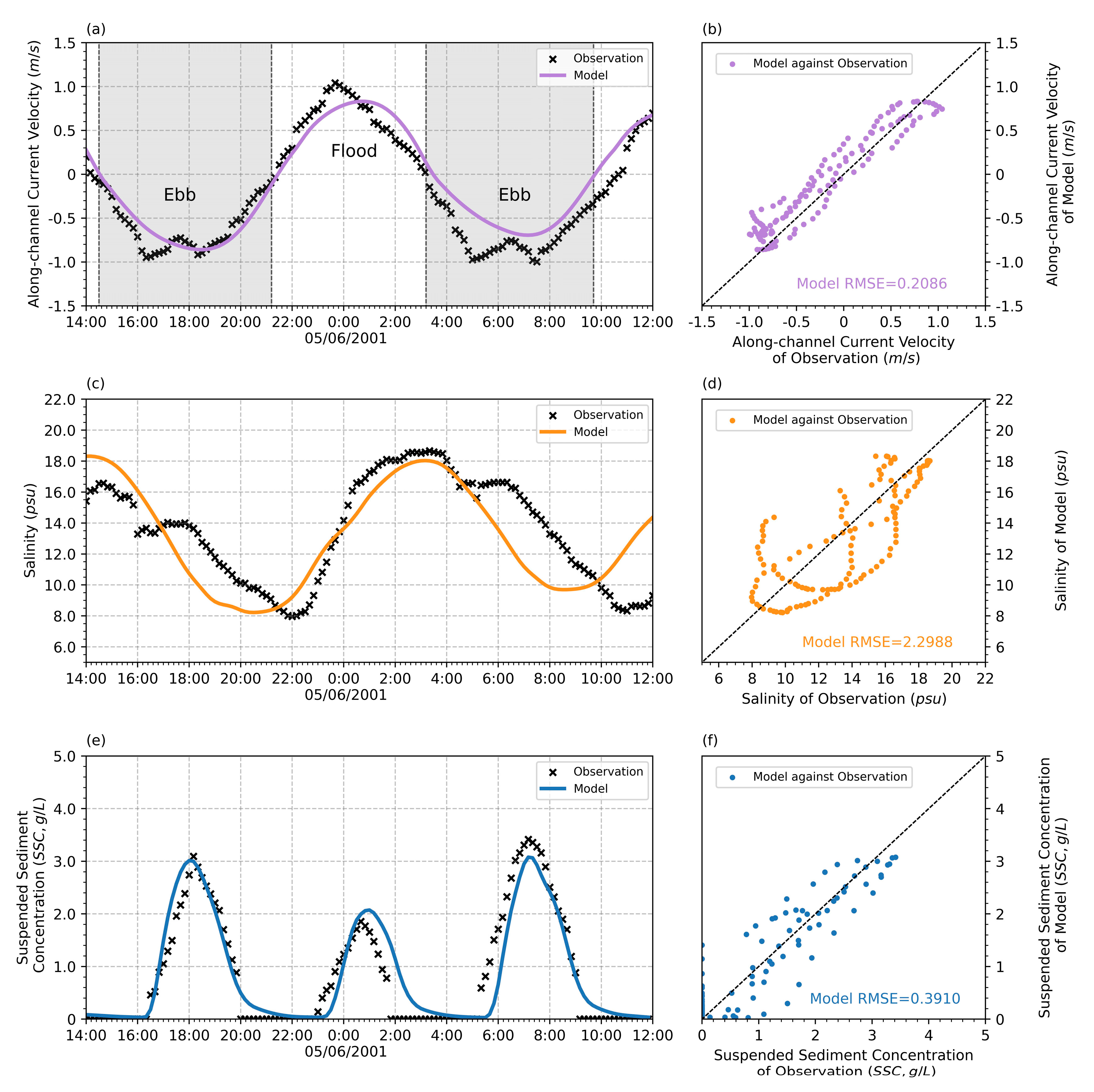
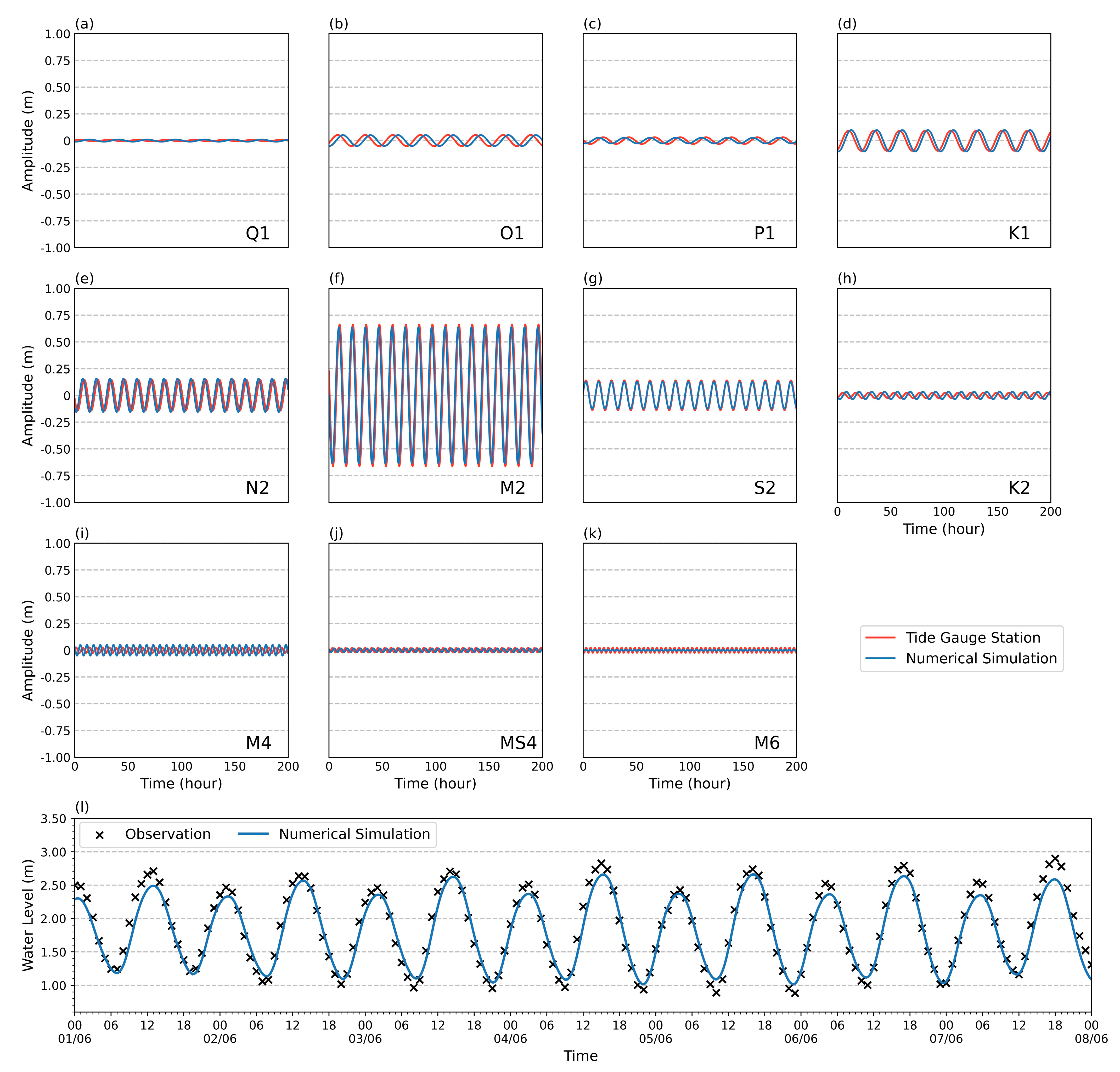
3.2. Validation of Salinity, Current Velocity, SSC, and Tides

The root-mean-square error (RMSE) and the correlation coefficient (CC) between the model and the observations are calculated to assess numerical simulation, defined as:

$$RMSE=\sqrt{\frac{{\sum }_{i=1}^n{(X_{obs,i}-X_{mod,i})}^2}{n}}$$

(9)

$$CC=\frac{{\sum }_{i=1}^n(X_{mod,i}-\overline{X_{mod}})(X_{obs,i}-\overline{X_{obs}})}{{[{\sum }_{i=1}^n{(X_{mod,i}-\overline{X_{mod}})}^2·{\sum }_{i=1}^n{(X_{obs,i}-\overline{X_{obs}})}^2]}^{\frac{1}{2}}}$$

(10)

Furthermore, based on the quantitative agreement between the model simulations and observations, the model skill (MS) is applied [67], defined as:

$$MS=1-\frac{{\sum }_{i=1}^n{\left|X_{mod,i}-X_{obs,i}\right|}^2}{{\sum }_{i=1}^n{(\left|X_{mod,i}-\overline{X_{obs}}\right|+\left|X_{obs,i}-\overline{X_{obs}}\right|)}^2}$$

(11)

The model skill is calculated based on the deviation between the model simulations and observations [67]. If this deviation is small, the model skill approaches 1, indicating high accuracy. Conversely, if the deviation is large, the ratio of the numerator to the denominator in the last term approaches equivalence, causing the model skill to approach 0 and indicating poor accuracy [68,69].

Figure 3 compares the simulation results of Exp00 against the observation around 5 June 2001. The simulated along-channel current velocity (the direction of the numerical grid extending from the southwest to the northeast in Figure 2c), bilinearly interpolated to S11 (triangle in Figure 2b), is in good agreement with the observed velocity (Figure 3a,b), with $RMSE=0.2086 \mathrm{m}/\mathrm{s},CC=0.9558,$ and $MS=0.9172$. The simulated salinity is also in good agreement with the observations, with $RMSE=2.2988 \mathrm{p}\mathrm{s}\mathrm{u},CC=0.7717,$ and $MS=0.8204$ (Figure 3c,d). Similarly, the model also simulates SSC well, with $RMSE=0.3910 \mathrm{g}/\mathrm{L},CC=0.9309,$ and $MS=0.9132$ (Figure 3e,f).

Figure 4l compares the simulated water level from the numerical simulation with the observation at tide gauge station ID 745 (star shape in Figure 2b). The RMSE is 0.1220 m, the CC is 0.9289, and the MS is 0.9349. The 11 total tidal constituents are obtained from both modeled and observed sea levels via harmonic analysis, as shown in Figure 4a–k, indicating that the model can simulate tidal constituents well. The five major tidal constituents (M2, S2, N2, K1, and O1) are evaluated by bias ($X_{mod}-X_{obs}$) and the absolute percentage error ($APE=\left|{(X}_{mod}-X_{obs})/X_{obs}\right|$) of amplitudes and phases. As shown in

Table 1. Comparison of amplitude and phase at tide gauge station ID 745 between observation and numerical simulation after harmonic analysis. Five tidal constituents (M2, S2, N2, O1, and K1) are listed in the table.

Tidal Constituent		M2	S2	N2	O1	K1	Average
Frequency (Hour−1)		0.0805	0.0833	0.0789	0.0387	0.0418
Amplitude (m)	Observation	0.6613	0.1390	0.1436	0.0517	0.0943
	Simulation	0.6359	0.1262	0.1546	0.0505	0.0998
	Bias	−0.0254	−0.0127	0.0110	−0.0012	0.0055
	APE	3.84%	9.17%	7.66%	2.34%	5.85%	5.77%
Phase(°)	Observation	289.8037	79.1998	256.7599	115.6710	156.9943
	Simulation	269.8934	73.3644	216.9272	183.1175	195.2466
	Bias	−19.9103	−5.8354	39.8327	67.4465	38.2523
	APE	5.53%	1.62%	11.06%	18.74%	10.63%	9.51%

, the amplitude bias of M2 is −0.0254 m (3.84%), and the phase bias is −19.91° (5.53%). The largest APE of amplitude is 9.17% for S2, and the largest APE of phase is 18.74% for K1. On average, the amplitude APE is 5.77% and the phase APE is 9.51%, indicating that tides are simulated well.

4. Assessment of the Spectrum-Based Scheme

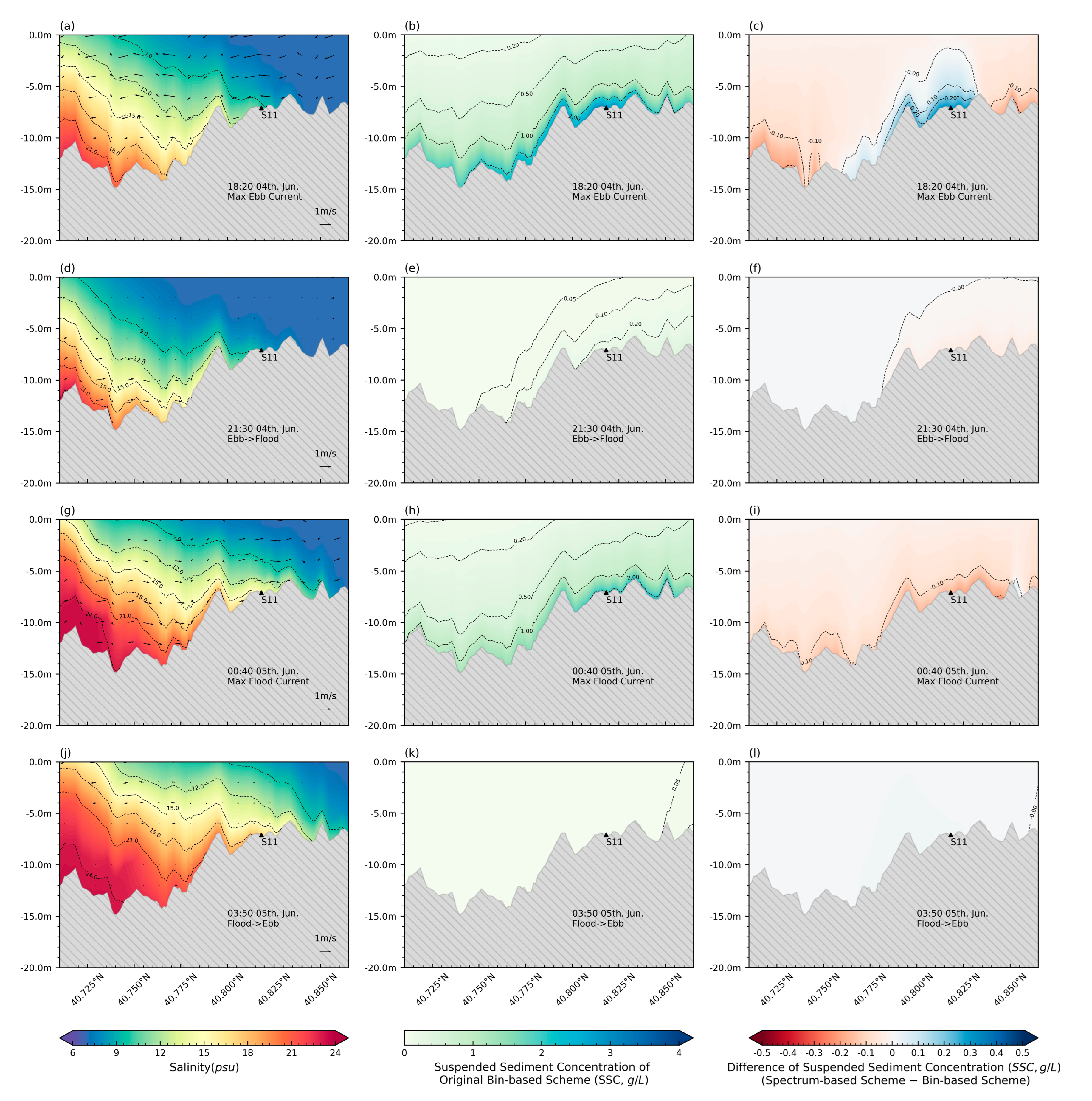
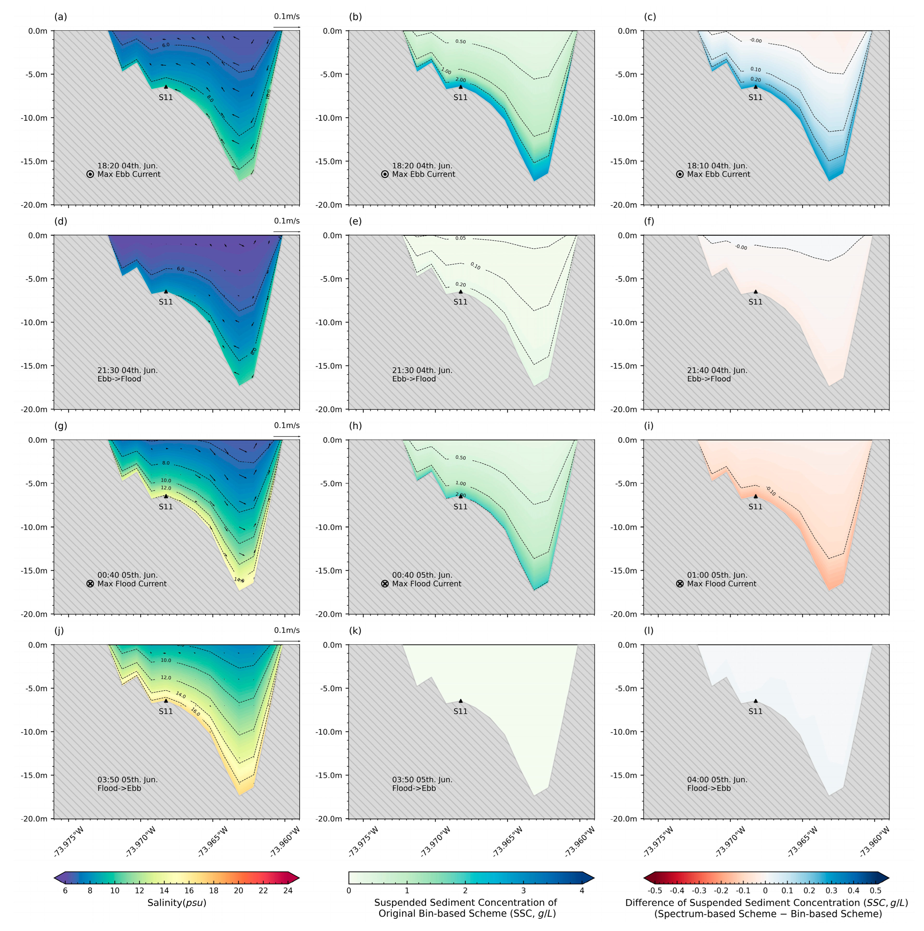
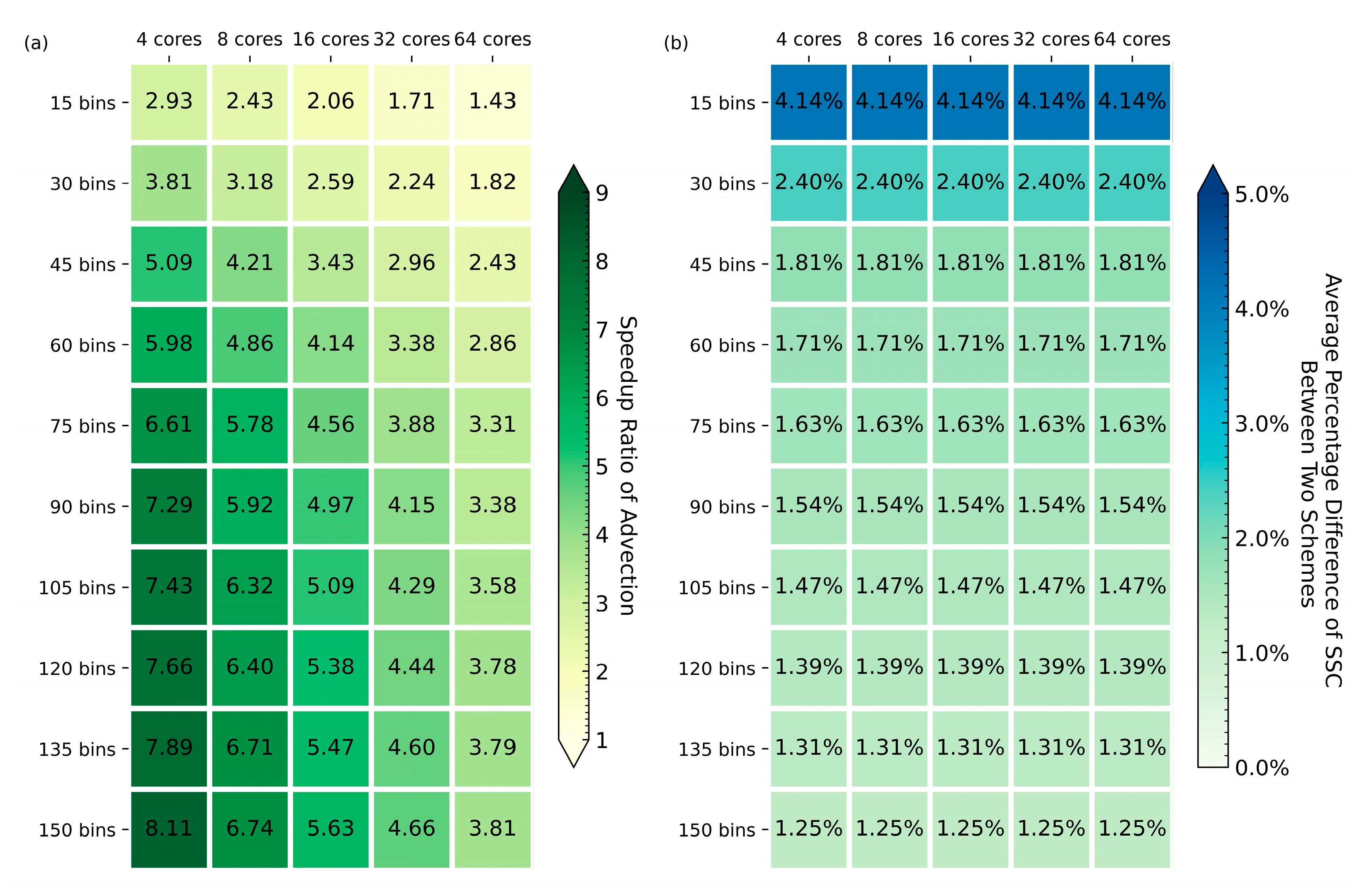
4.1. Comparison of SSC between the Bin-Based Scheme and the Spectrum-Based Scheme

Figure 5 shows the along-channel distribution from Exp00 (with the bin-based scheme) and the differences between Exp00 and Exp01 (with the spectrum-based scheme). At max ebb current, seaward flow velocity reaches its maximum (Figure 5a), resulting in increased bottom boundary shear stress that tends to resuspend fine-grained sediments, and SSC increases vertically from top to bottom with about 3 g/L near the bed (Figure 5b), where the differences (Figure 5c) can be about 0.24 g/L (8.20%) at S11. At slack tide after ebb, near the low tide, the flow velocity is near zero, SSC decreases to about 0.1 g/L due to settling (Figure 5e), and the differences are near zero (Figure 5f). At max flood current, near mid-tide levels, the landward flow velocity is at its maximum (Figure 5g), again resulting in increased bottom boundary shear stress that tends to resuspend sediments, and SSC is high again, reaching about 2 g/L near the bed (Figure 5h), where the differences (Figure 5i) are up to 0.08 g/L (3.94%). At slack tide after flood, near the high tide, the flow velocity is near zero, and SSC and the corresponding differences (Figure 5k–l) are both around zero. Similarly, Figure 6 shows the distribution in the cross-channel direction and the differences between Exp00 and Exp01. At max ebb current, the seaward flow velocity is at its maximum (Figure 6a), and SSC increases vertically from top to bottom, recording about 3 g/L near the bed (Figure 6b). Meanwhile, bias also increases vertically (Figure 6c). At slack tide after ebb, SSC is about 0.1 g/L (Figure 6e) and bias is near zero (Figure 6f); at max flood current, landward flow velocity is at its maximum and SSC increases vertically from top to bottom, recording about 2 g/L near the bed (Figure 6h). Meanwhile, bias also increases vertically (Figure 6i). At slack tide after flood, SSC and bias are both around zero (Figure 6k–l). The differences vary with the hydrodynamic conditions. During periods when the current velocity reaches its maximum, the differences between the bin-based scheme and the spectrum-based scheme tend to become larger, attributed to the increased complexity of more sediment transport processes under high-flow conditions. Conversely, during periods when the current velocity is minimal, the differences become smaller, because the reduced flow simplifies the sediment dynamics. Overall, the average differences over the tidal cycle are about 2.40% between the original bin-based scheme and the new spectrum-based scheme, where the largest differences occur near the riverbed during the maximum current.

The S11 site (triangle in Figure 2b) is a crucial location within the Hudson River estuary for understanding sediment dynamics. According to Traykovski et al. [33], the S11 site provides significant insights into how sediment trapping is influenced by the interaction of frontal convergence and lateral circulation processes. This interaction leads to a pattern of intensified sediment trapping, which is vital for comprehending sediment transport mechanisms within the estuary. This makes S11 an ideal location of validation for the spectrum-based scheme in numerical simulation.

Figure 7a,b compares the time series of SSC from Exp00 and Exp01 with the observed value at S11. The RMSE from Exp01 is 0.4139 g/L, about 0.0229 g/L larger than that from Exp00 and increased by about 5.85%. Figure 7c–e shows the fitted spectral shape from the distribution at different times (taking 18:00 on 4 June, 01:00 on 5 June, and 07:00 on 5 June as examples). The variation in tides impacts the suspended sediments. The higher tidal current velocity observed during these times correlates with increased sediment resuspension; meanwhile, the fitted parameters $\widehat{m},\widehat{\mu },$and $\widehat{\sigma }$ vary with the change in the SSC distribution, and the corresponding difference (percentage difference) is 0.06 g/L (2.08%), 0.11 g/L (5.57%), and 0.05 g/L (1.89%), respectively. Overall, the distribution can be captured well by employing the spectrum-based scheme.

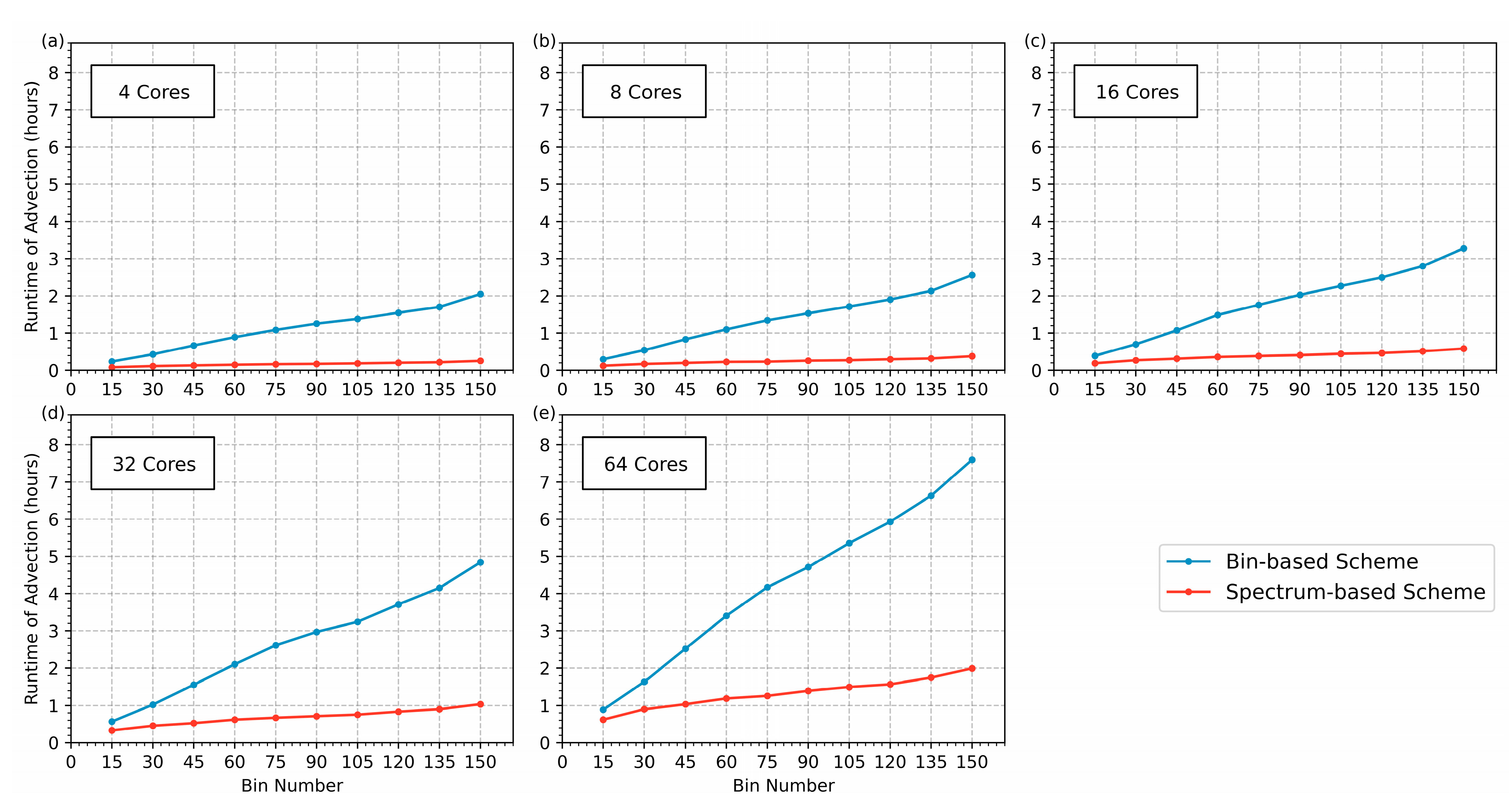
4.2. Evaluation of the Runtime of the Spectrum-Based Scheme

Figure 8 compares the runtime of advection based on the bin-based scheme and the spectrum-based scheme for the different number of bins (ranging from 15 to 150) and the number of parallel cores (ranging from 4 to 64). The speedup ratio, the runtime of the bin-based scheme divided by the spectrum-based scheme, is calculated (Figure 9a) for all experiments (Table A1). The runtime of advection with the spectrum-based scheme (red lines in Figure 8) is always lower than with the bin-based scheme (blue lines in Figure 8), indicating that the spectrum-based scheme can significantly save the model runtime.

Figure 9 shows the speedup ratios and the average percentage differences of the 50 paired experiments. With a fixed number of bins, the increase in the number of parallel cores will cause a decrease in the speedup ratio (rows in Figure 9a), and the average percentage difference remains the same (rows in Figure 9b). With a fixed number of parallel cores, the increase in the number of bins will cause an increase in the speedup ratio (columns in Figure 9a) due to only three parameters being used in the spectrum-based scheme, and it will cause a decrease in the average percentage difference (columns in Figure 9b), since a greater number of bins tends to produce a more accurate spectral distribution. On average, among all 50 paired experiments, the average percentage difference is 1.86% and the speedup ratio is 4.51 times. The maximum speedup ratio is achieved with 4 cores and 150 bins (Figure 8a and Figure 9). The runtime decreases from 2.05 h to 0.25 h, with a reduction of 1.80 h (the speedup ratio is 8.11). In summary, the spectrum-based scheme can accelerate the model remarkably and has the potential to be applied to the simulation for fine-grained sediments in estuaries.

5. Conclusions and Discussion

This study develops a new spectrum-based scheme for a size-resolved flocculation module to improve the computational efficiency of modeling fine-grained sediment transport in estuaries.

The spectrum-based scheme, fitting the discrete size bins into the substantial spectral distribution, can accelerate the numerical model. The scheme is applied for simulation in the Hudson River estuary, validated by observations. Fifty paired experiments with different bin numbers and parallel core numbers are conducted. The results indicate the spectrum-based scheme can save the model runtime without introducing large bias. Notably, acceleration is achieved with the increase in bin number and the decrease in parallel core number. On average, the spectrum-based scheme accelerates the advection by 4.51 times while maintaining a low average difference of 1.86%.

The 50 paired experiments reveal that other sedimentary processes (e.g., flocculation) also significantly impact the overall runtime. Figure 10 shows the overall runtime between the two schemes. Taking the 16 cores (Figure 10a) and 64 cores (Figure 10b) as examples, the average proportion of runtime for advection to overall runtime is 20.30% with 16 cores (41.26% with 64 cores). Meanwhile, the average proportion of reduced runtime to total runtime is 15.14% with 16 cores (27.17% with 64 cores). Future enhancements could involve building upon the foundation of a new purely spectrum-based scheme, potentially resulting in more significant acceleration.

The spectrum-based scheme is based on the coupling of a size-resolved flocculation module in sbPOM. Meanwhile, analogous size-resolved modules are present in other ocean models [26,28], such as the Regional Ocean Modeling System (ROMS). This suggests the potential for the spectrum-based scheme to be applied to other models. Moreover, this spectrum-based scheme holds potential for practical applications. For example, it can be utilized to justify different sedimentation rates in estuaries and salt marsh restoration.

In reality, each estuary possesses unique characteristics. The effectiveness of the spectrum-based scheme is contingent upon the distribution of fine-grained sediments in the estuary. If the spectrum exhibits bimodal or multimodal peak patterns, the spectrum-based scheme needs to be improved to fit the local distribution. Areas with heterogeneous sediment types introduce additional variability for numerical simulation. This variability can affect the accuracy; future research might consider incorporating more detailed sediment characterization to enhance the model. Flood episodes present unique challenges for sediment transport modeling due to the significant alterations in water volume and flow velocity, which may change the sediment dynamics. Future research is warranted.

References

1. Elliott, M.; Whitfield, A.K. Challenging paradigms in estuarine ecology and management. Estuar. Coast. Shelf Sci. 2011, 94, 306–314. [Google Scholar] [CrossRef]
2. Thrush, S.F.; Townsend, M.; Hewitt, J.E.; Davies, K.; Lohrer, A.M.; Lundquist, C.; Cartner, K.; Dymond, J. The many uses and values of estuarine ecosystems. In Ecosystem Services in New Zealand–Conditions Trends; Manaaki Whenua Press: Lincoln, New Zealand, 2013; pp. 226–237. [Google Scholar]
3. Hoque, M.Z.; Cui, S.; Islam, I.; Xu, L.; Tang, J. Future impact of land use/land cover changes on ecosystem services in the lower meghna river estuary, Bangladesh. Sustainability 2020, 12, 2112. [Google Scholar] [CrossRef]
4. Rakib, M.R.J.; Hossain, M.B.; Kumar, R.; Ullah, M.A.; Al Nahian, S.; Rima, N.N.; Choudhury, T.R.; Liba, S.I.; Yu, J.; Khandaker, M.U. Spatial distribution and risk assessments due to the microplastics pollution in sediments of Karnaphuli River Estuary, Bangladesh. Sci. Rep. 2022, 12, 8581. [Google Scholar] [CrossRef]
5. Wang, Z.; Lin, K.; Liu, X. Distribution and pollution risk assessment of heavy metals in the surface sediment of the intertidal zones of the Yellow River Estuary, China. Mar. Pollut. Bull. 2022, 174, 113286. [Google Scholar] [CrossRef]
6. Ballagh, F.E.A.; Rabouille, C.; Andrieux-Loyer, F.; Soetaert, K.; Elkalay, K.; Khalil, K. Spatio-temporal dynamics of sedimentary phosphorus along two temperate eutrophic estuaries: A data-modelling approach. Cont. Shelf Res. 2020, 193, 104037. [Google Scholar] [CrossRef]
7. Ho, Q.N.; Fettweis, M.; Spencer, K.L.; Lee, B.J. Flocculation with heterogeneous composition in water environments: A review. Water Res. 2022, 213, 118147. [Google Scholar] [CrossRef] [PubMed]
8. Zhao, C.; Zhou, J.; Yan, Y.; Yang, L.; Xing, G.; Li, H.; Wu, P.; Wang, M.; Zheng, H. Application of coagulation/flocculation in oily wastewater treatment: A review. Sci. Total Environ. 2021, 765, 142795. [Google Scholar] [CrossRef] [PubMed]
9. Vercruysse, K.; Grabowski, R.C.; Rickson, R.J. Suspended sediment transport dynamics in rivers: Multi-scale drivers of temporal variation. Earth-Sci. Rev. 2017, 166, 38–52. [Google Scholar] [CrossRef]
10. Burchard, H.; Schuttelaars, H.M.; Ralston, D.K. Sediment trapping in estuaries. Annu. Rev. Mar. Sci. 2018, 10, 371–395. [Google Scholar] [CrossRef]
11. Choi, Y.E.; Oh, C.-O.; Chon, J. Applying the resilience principles for sustainable ecotourism development: A case study of the Nakdong Estuary, South Korea. Tour. Manag. 2021, 83, 104237. [Google Scholar] [CrossRef]
12. Mitchell, S. Turbidity maxima in four macrotidal estuaries. Ocean Coast. Manag. 2013, 79, 62–69. [Google Scholar] [CrossRef]
13. McManus, J. Salinity and suspended matter variations in the Tay estuary. Cont. Shelf Res. 2005, 25, 729–747. [Google Scholar] [CrossRef]
14. Wang, H.; Yang, Z.; Li, Y.; Guo, Z.; Sun, X.; Wang, Y. Dispersal pattern of suspended sediment in the shear frontal zone off the Huanghe (Yellow River) mouth. Cont. Shelf Res. 2007, 27, 854–871. [Google Scholar] [CrossRef]
15. McAnally, W.H.; Friedrichs, C.; Hamilton, D.; Hayter, E.; Shrestha, P.; Rodriguez, H.; Sheremet, A.; Teeter, A.; Mud, A.T.C.o.M.o.F. Management of fluid mud in estuaries, bays, and lakes. I: Present state of understanding on character and behavior. J. Hydraul. Eng. 2007, 133, 9–22. [Google Scholar] [CrossRef]
16. Winterwerp, J.; Kranenburg, C. Erosion of fluid mud layers. II: Experiments and model validation. J. Hydraul. Eng. 1997, 123, 512–519. [Google Scholar] [CrossRef]
17. Manning, A.; Langston, W.; Jonas, P. A review of sediment dynamics in the Severn Estuary: Influence of flocculation. Mar. Pollut. Bull. 2010, 61, 37–51. [Google Scholar] [CrossRef] [PubMed]
18. Partheniades, E. A fundamental framework for cohesive sediment dynamics. Estuar. Cohesive Sediment Dyn. 1986, 14, 219–250. [Google Scholar] [CrossRef]
19. Meakin, P. Formation of fractal clusters and networks by irreversible diffusion-limited aggregation. Phys. Rev. Lett. 1983, 51, 1119. [Google Scholar] [CrossRef]
20. Ladd, A.J.; Verberg, R. Lattice-Boltzmann simulations of particle-fluid suspensions. J. Stat. Phys. 2001, 104, 1191–1251. [Google Scholar] [CrossRef]
21. Teisson, C. Cohesive suspended sediment transport: Feasibility and limitations of numerical modeling. J. Hydraul. Res. 1991, 29, 755–769. [Google Scholar] [CrossRef]
22. Krishnappan, B.G. Review of a semi-empirical modelling approach for cohesive sediment transport in river systems. Water 2022, 14, 256. [Google Scholar] [CrossRef]
23. Nicholson, J.; O’Connor, B.A. Cohesive sediment transport model. J. Hydraul. Eng. 1986, 112, 621–640. [Google Scholar] [CrossRef]
24. Xu, F.; Wang, D.-P.; Riemer, N. Modeling flocculation processes of fine-grained particles using a size-resolved method: Comparison with published laboratory experiments. Cont. Shelf Res. 2008, 28, 2668–2677. [Google Scholar] [CrossRef]
25. Sherwood, C.R.; Aretxabaleta, A.L.; Harris, C.K.; Rinehimer, J.P.; Verney, R.; Ferré, B. Cohesive and mixed sediment in the regional ocean modeling system (ROMS v3. 6) implemented in the Coupled Ocean–Atmosphere–Wave–Sediment Transport Modeling System (COAWST r1234). Geosci. Model Dev. 2018, 11, 1849–1871. [Google Scholar] [CrossRef]
26. Verney, R.; Lafite, R.; Brun-Cottan, J.C.; Le Hir, P. Behaviour of a floc population during a tidal cycle: Laboratory experiments and numerical modelling. Cont. Shelf Res. 2011, 31, S64–S83. [Google Scholar] [CrossRef]
27. Teh, C.Y.; Budiman, P.M.; Shak, K.P.Y.; Wu, T.Y. Recent advancement of coagulation–flocculation and its application in wastewater treatment. Ind. Eng. Chem. Res. 2016, 55, 4363–4389. [Google Scholar] [CrossRef]
28. Liu, J.; Liang, J.H.; Xu, K.; Chen, Q.; Ozdemir, C.E. Modeling sediment flocculation in Langmuir turbulence. J. Geophys. Res. Ocean. 2019, 124, 7883–7907. [Google Scholar] [CrossRef]
29. Tarpley, D.R.; Harris, C.K.; Friedrichs, C.T.; Sherwood, C.R. Tidal variation in cohesive sediment distribution and sensitivity to flocculation and bed consolidation in an idealized, partially mixed estuary. J. Mar. Sci. Eng. 2019, 7, 334. [Google Scholar] [CrossRef]
30. Figueroa, S.M.; Lee, G.h.; Chang, J.; Jung, N.W. Impact of estuarine dams on the estuarine parameter space and sediment flux decomposition: Idealized numerical modeling study. J. Geophys. Res. Ocean. 2022, 127, e2021JC017829. [Google Scholar] [CrossRef]
31. Bott, A. A flux method for the numerical solution of the stochastic collection equation. J. Atmos. Sci. 1998, 55, 2284–2293. [Google Scholar] [CrossRef]
32. Thorn, M. 6 Physical processes of siltation in tidal channels. In Hydraulic Modelling in Maritime Engineering; Thomas Telford Publishing: London, UK, 1982; pp. 65–73. [Google Scholar]
33. Traykovski, P.; Geyer, R.; Sommerfield, C. Rapid sediment deposition and fine-scale strata formation in the Hudson estuary. J. Geophys. Res. Earth Surf. 2004, 109, F02004. [Google Scholar] [CrossRef]
34. Xu, F.; Wang, D.-P.; Riemer, N. An idealized model study of flocculation on sediment trapping in an estuarine turbidity maximum. Cont. Shelf Res. 2010, 30, 1314–1323. [Google Scholar] [CrossRef]
35. Smoluchowski, M. Mathematical theory of the kinetics of the coagulation of colloidal solutions. Z. Phys. Chem. 1917, 92, 129–168. [Google Scholar]
36. Burd, A.; Jackson, G. Predicting particle coagulation and sedimentation rates for a pulsed input. J. Geophys. Res. Ocean. 1997, 102, 10545–10561. [Google Scholar] [CrossRef]
37. Maggi, F. Flocculation Dynamics of Cohesive Sediment; Faculty of Civil Engineering and Geosciences, Delft University of Technology: Delft, The Netherlands, 2005. [Google Scholar]
38. Hill, P.S.; Voulgaris, G.; Trowbridge, J.H. Controls on floc size in a continental shelf bottom boundary layer. J. Geophys. Res. Ocean. 2001, 106, 9543–9549. [Google Scholar] [CrossRef]
39. Sternberg, R.; Berhane, I.; Ogston, A. Measurement of size and settling velocity of suspended aggregates on the northern California continental shelf. Mar. Geol. 1999, 154, 43–53. [Google Scholar] [CrossRef]
40. Leussen, V. Estuarine Macroflocs and Their Role in Fine-Grained Sediment Transport. Ph. D. Thesis, University of Utrecht, Utrecht, The Netherlands, 1994.
41. McCave, I. Size spectra and aggregation of suspended particles in the deep ocean. Deep Sea Res. Part A Oceanogr. Res. Pap. 1984, 31, 329–352. [Google Scholar] [CrossRef]
42. Winterwerp, J.C. A simple model for turbulence induced flocculation of cohesive sediment. J. Hydraul. Res. 1998, 36, 309–326. [Google Scholar] [CrossRef]
43. Zhang, J.j.; Li, X.y. Modeling particle-size distribution dynamics in a flocculation system. AIChE J. 2003, 49, 1870–1882. [Google Scholar] [CrossRef]
44. Hall, A.R. Generalized method of moments. In A Companion to Theoretical Econometrics; Blackwell Publishing Ltd.: Oxford, UK, 2003; pp. 230–255. [Google Scholar] [CrossRef]
45. Imbens, G.W. Generalized method of moments and empirical likelihood. J. Bus. Econ. Stat. 2002, 20, 493–506. [Google Scholar] [CrossRef]
46. Jordi, A.; Wang, D.-P. sbPOM: A parallel implementation of Princenton Ocean Model. Environ. Model. Softw. 2012, 38, 59–61. [Google Scholar] [CrossRef]
47. Nitsche, F.; Ryan, W.; Carbotte, S.; Bell, R.; Slagle, A.; Bertinado, C.; Flood, R.; Kenna, T.; McHugh, C. Regional patterns and local variations of sediment distribution in the Hudson River Estuary. Estuar. Coast. Shelf Sci. 2007, 71, 259–277. [Google Scholar] [CrossRef]
48. Sinsabaugh, R.; Findlay, S. Microbial production, enzyme activity, and carbon turnover in surface sediments of the Hudson River estuary. Microb. Ecol. 1995, 30, 127–141. [Google Scholar] [CrossRef] [PubMed]
49. Geyer, W.R.; Woodruff, J.D.; Traykovski, P. Sediment transport and trapping in the Hudson River estuary. Estuaries 2001, 24, 670–679. [Google Scholar] [CrossRef]
50. Blumberg, A.F.; Mellor, G.L. A description of a three-dimensional coastal ocean circulation model. Three-Dimens. Coast. Ocean Models 1987, 4, 1–16. [Google Scholar] [CrossRef]
51. Chau, K.-W. Manipulation of numerical coastal flow and water quality models. Environ. Model. Softw. 2003, 18, 99–108. [Google Scholar] [CrossRef]
52. Vichi, M.; Pinardi, N.; Zavatarelli, M.; Matteucci, G.; Marcaccio, M.; Bergamini, M.; Frascari, F. One-dimensional ecosystem model tests in the Po Prodelta area (Northern Adriatic Sea). Environ. Model. Softw. 1998, 13, 471–481. [Google Scholar] [CrossRef]
53. Liu, X.; Huang, W. Modeling sediment resuspension and transport induced by storm wind in Apalachicola Bay, USA. Environ. Model. Softw. 2009, 24, 1302–1313. [Google Scholar] [CrossRef]
54. Mellor, G.L.; Yamada, T. Development of a turbulence closure model for geophysical fluid problems. Rev. Geophys. 1982, 20, 851–875. [Google Scholar] [CrossRef]
55. Nittis, K.; Perivoliotis, L.; Korres, G.; Tziavos, C.; Thanos, I. Operational monitoring and forecasting for marine environmental applications in the Aegean Sea. Environ. Model. Softw. 2006, 21, 243–257. [Google Scholar] [CrossRef]
56. Sun, Z.; Shao, W.; Yu, W.; Li, J. A study of wave-induced effects on sea surface temperature simulations during typhoon events. J. Mar. Sci. Eng. 2021, 9, 622. [Google Scholar] [CrossRef]
57. Ralston, D.K.; Geyer, W.R. Episodic and long-term sediment transport capacity in the Hudson River estuary. Estuaries Coasts 2009, 32, 1130–1151. [Google Scholar] [CrossRef]
58. Zhu, Y.; Lu, J.; Liao, H.; Wang, J.; Fan, B.; Yao, S. Research on cohesive sediment erosion by flow: An overview. Sci. China Ser. E Technol. Sci. 2008, 51, 2001–2012. [Google Scholar] [CrossRef]
59. Yang, M.-Q.; Wang, G.-L. The incipient motion formulas for cohesive fine sediments. J. Basic Sci. Eng. 1995, 3, 99–109. [Google Scholar]
60. Carrere, L.; Lyard, F.; Cancet, M.; Guillot, A. FES 2014, a new tidal model on the global ocean with enhanced accuracy in shallow seas and in the Arctic region. In Proceedings of the EGU General Assembly Conference Abstracts, Vienna, Austria, 12–17 April 2015; p. 5481. [Google Scholar]
61. Lyard, F.H.; Allain, D.J.; Cancet, M.; Carrère, L.; Picot, N. FES2014 global ocean tide atlas: Design and performance. J. Ocean Sci. 2021, 17, 615–649. [Google Scholar] [CrossRef]
62. Caldwell, P.; Merrifield, M.; Thompson, P. Sea level measured by tide gauges from global oceans–the Joint Archive for Sea Level holdings (NCEI Accession 0019568), Version 5.5, NOAA National Centers for Environmental Information. Cent. Environ. Inf. Dataset 2015, 10, V5V40S47W. [Google Scholar]
63. Bayliss, A.; Turkel, E. Radiation boundary conditions for wave-like equations. Commun. Pure Appl. Math. 1980, 33, 707–725. [Google Scholar] [CrossRef]
64. Marchesiello, P.; McWilliams, J.C.; Shchepetkin, A. Open boundary conditions for long-term integration of regional oceanic models. Ocean Model. 2001, 3, 1–20. [Google Scholar] [CrossRef]
65. Smolarkiewicz, P.K. A fully multidimensional positive definite advection transport algorithm with small implicit diffusion. J. Comput. Phys. 1984, 54, 325–362. [Google Scholar] [CrossRef]
66. Smagorinsky, J. The dynamical influence of large-scale heat sources and sinks on the quasi-stationary mean motions of the atmosphere. Q. J. R. Meteorol. Soc. 1953, 79, 342–366. [Google Scholar] [CrossRef]
67. Willmott, C.J. On the validation of models. Phys. Geogr. 1981, 2, 184–194. [Google Scholar] [CrossRef]
68. Warner, J.C.; Geyer, W.R.; Lerczak, J.A. Numerical modeling of an estuary: A comprehensive skill assessment. J. Geophys. Res. Ocean. 2005, 110, C05001. [Google Scholar] [CrossRef]
69. Gu, C.; Li, H.; Xu, F.; Cheng, P.; Wang, X.H.; Xu, S.; Peng, Y. Numerical study of Jiulongjiang river plume in the wet season 2015. Reg. Stud. Mar. Sci. 2018, 24, 82–96. [Google Scholar] [CrossRef]
Figure 1. Schematic diagrams of the fitted spectral shape (red solid line) using the spectrum-based scheme, and the observed spectral shape (black dashed line) of sediment size distribution in (a) the Brisbane estuary, Australia; (b) the Grangemouth estuary, Scotland; and (c) the Belawan estuary, Indonesia.
Jmse 12 01189 g001
Figure 2. (a) A topographic map of the Hudson River; (b) a topographic map of the New York Harbor, including our study area, the Hudson River estuary; (c) 32 × 128 grid for the numerical model in the horizontal direction.
Jmse 12 01189 g002
Figure 3. Time series of model simulation and observation at S11 (triangle in Figure 2b) of (a) along-channel current velocity, (c) salinity, (e) suspended sediment concentration (SSC), and (b,d,f) the corresponding scatterplots.
Jmse 12 01189 g003
Figure 4. Time series of harmonic analysis for model (blue) and observation (red) at tide gauge station ID 745 (star shape in Figure 2b), with (ad) diurnal tidal constituents Q1, O1, P1, and K1; (eh) semidiurnal tidal constituents N2, M2, S2, and K2; and (ik) shallow water constituents M4, MS4, and M6. (l) Time series of synthesized water level of model simulation (blue) and observation (black scatter).
Jmse 12 01189 g004
Figure 5. Along-channel distribution of salinity and velocity at (a) max ebb current, (d) slack tide after ebb, (g) max flood current, and (j) slack tide after flood. Note that the magnitude of vertical velocity is exaggerated 100 times for ease of visualization. Along-channel distribution of SSC at (b) max ebb current, (e) slack tide after ebb, (h) max flood current, (k) slack tide after flood, and (c,f,i,l) the corresponding differences between the spectrum-based scheme and the bin-based scheme.
Jmse 12 01189 g005
Figure 6. Cross-channel distribution of salinity and velocity at (a) max ebb current, (d) slack tide after ebb, (g) max flood current, and (j) slack tide after flood. Note that the magnitude of vertical velocity is exaggerated 100 times for ease of visualization. Cross-channel distribution of SSC at (b) max ebb current, (e) slack tide after ebb, (h) max flood current, (k) slack tide after flood, and (c,f,i,l) the corresponding differences between the spectrum-based scheme and the bin-based scheme.
Jmse 12 01189 g006
Figure 7. (a) Time series of SSC at S11 from Exp00 (modeled with the bin-based scheme, blue dashed line), Exp01 (modeled with the spectrum-based scheme, red dashed line), and observation (black scatter) and (b) the corresponding scatterplot. Comparison of the discrete distribution (blue bar) from Exp00 and the corresponding fitted spectrum (red solid line) from Exp01 at S11 at (c) 18:00 on 4 June, (d) 01:00 on 5 June, and (e) 07:00 on 5 June.
Jmse 12 01189 g007
Figure 8. Comparison of the runtime of advection between the bin-based scheme (blue) and the spectrum-based scheme (red) across different bin numbers (ranging from 15 to 150) with parallel scale for (a) 4 cores, (b) 8 cores, (c) 16 cores, (d) 32 cores, and (e) 64 cores.
Jmse 12 01189 g008
Figure 9. Heatmaps of 50 paired experiments between the bin-based scheme and the spectrum-based scheme across different bin numbers and different parallel core numbers of (a) the speedup ratio of advection and (b) the average percentage differences.
Jmse 12 01189 g009
Figure 10. Comparison of overall runtime between the bin-based scheme (slash) and the spectrum-based scheme (backslash) across different bin numbers (ranging from 15 to 150) with the parallel scale of (a) 16 cores and (b) 64 cores. The blue blocks represent the runtime of advection; the pink blocks represent the runtime of other sedimentary processes, including flocculation, settling, diffusion, etc.; and the red blocks represent the runtime of hydrodynamic calculation and other read/write (input/output) operations.
Jmse 12 01189 g010