Multidisciplinary Design Optimization of Underwater Vehicles Based on a Combined Proxy Model

Abstract

To improve the efficiency of the multidisciplinary design optimization of underwater vehicles, this paper proposes a combined proxy model with adaptive dynamic sampling. The radial basis function model (RBF), Kriging model, and polynomial response surface model (PRS) are used to construct the proxy model. Efficient sample points are collected based on the synthetic minority oversampling technique (SMOTE) algorithm and the lower confidence bound (LCB) criterion. The proxy model process is integrated after dynamic sampling. The collaborative optimization framework is used, which considers the coupling between the main system set and the subsystem set. The hierarchical analysis method is used to transform the multidisciplinary optimization problem into a single-objective optimization problem. Computational fluid dynamics (CFD) numerical simulation is utilized to simulate underwater submarine navigation. The optimization strategy is applied to the underwater vehicle SUBOFF to optimize resistance and energy consumption. Three dynamic proxy models and three static proxy models are compared. The results show that the optimization efficiency of the underwater vehicle has been improved. To prove the generalization performance of the proposed combined proxy model, a reducer example is investigated for comparison. The results show that the combined proxy model (CPM) is highly accurate and has excellent generalization performance.

1. Introduction

CFD numerical simulation can be used to analyze the hydrodynamic performance of underwater vehicles. However, the time-consuming characteristics of numerical simulation hinder efficiency when applied to the optimization design of an underwater vehicle. To solve this problem, a proxy model provides an effective way. Typical high-fidelity proxy models include the radial basis function model (RBF), Kriging model, polynomial response surface model (PRS), artificial neural network model (ANN), support vector machine model, etc. In the early stages, researchers used a static proxy model. Due to the complexity of engineering problems and the need for technical support, the static proxy model is inadequate to meet the requirements. Therefore, research on a dynamic proxy model is required. Long et al. [1,2] proposed a dynamic proxy model based on the lower confidence bound (LCB) criterion sampling method and utilized the physical expectation method to conduct multidisciplinary design optimization for the aircraft. Diez Silvia et al. [3] proposed a dynamic proxy model based on an adaptive sampling method, while Su et al. [4] proposed a dynamic proxy model based on the Monte Carlo simulation method, effectively addressing the complex instability issue. Luo et al. [5] proposed a dynamic proxy model based on an annealing algorithm for multidisciplinary route optimization of underwater vehicles. Pan and Luo [6] proposed a dynamic proxy model based on the synthetic minority oversampling technique (SMOTE) algorithm and compared it with several other dynamic proxy models, demonstrating the effectiveness of the SMOTE algorithm. Although a dynamic proxy model shows high effectiveness in improving the efficiency of sampling points, it is unable to adapt to multiple engineering problems. Geol et al. [7] proposed a combined proxy model, which utilizes weights to combine multiple proxy models. The results show the fitting accuracy of the combined proxy model and good generalization performance. Lee and Choi [8] proposed a new weight distribution method by utilizing cross-validation errors. Chen et al. [9] introduced adaptive functions and proposed an adaptive weight distribution method. Yang et al. [10] utilized a combined proxy model to conduct multidisciplinary design optimization for complex engineering problems. The combined proxy model exhibits high fitting accuracy and the capability to address complex engineering problems. However, it often necessitates a very high computing cost. The proxy model that combines efficiency and generalization performance reflects its importance. The purpose of a new proxy model is to solve increasingly complex engineering problems.

In the field of underwater vehicle optimization under complex sea conditions, many studies have been conducted. At the stage of schematic design, multidisciplinary design optimization (MDO) was preferred [11,12]. Static proxy models to optimize the multidisciplinary design of the underwater vehicle are utilized and incorporated into MDO [13,14,15]. To improve the optimization efficiency, Luo et al. [5] used a dynamic proxy model to optimize the multidisciplinary design of the underwater vehicle. Furthermore, Pan and Luo [6] utilized a dynamic proxy model to design a lightweight and fast underwater vehicle. Previous studies have demonstrated the feasibility of dynamic sampling applied to underwater vehicles. However, research on enhancing generalization performance in the multidisciplinary design optimization of underwater vehicles remains limited, especially for the multidisciplinary design optimization of underwater vehicles, which improves both generalization performance and efficiency. The dynamic processing of sampling points, which involves coupling multiple disciplines and proxy models, is challenging. This challenge stems from the technical difficulty of achieving the simultaneous convergence of three proxy models. To solve the above problem, in this paper, the framework of collaborative optimization and the analytic hierarchy process (AHP) are used to consider the coupling relationship between the main subject set and the sub-subject set. The multidisciplinary target problem is transformed into a single target optimization problem. The SMOTE algorithm is employed to efficiently interpolate the crucial sample points, generating efficient sample points to ensure the fitting of high-fidelity proxy model samples. This approach enables the proxy model to converge even with fewer sample points. The sampling method is applied to the radial basis function (RBF), Kriging, and polynomial response surface (PRS) models, respectively. Based on the adaptive interpolation of key sample points, each set of sample points is dynamically updated. The NSGA-II genetic algorithm is used to optimize the underwater vehicle. The results demonstrate the rapid convergence of the algorithm. A total of 10% to 20% of the total sample is taken as the convergence judgment sample size. The SMOTE algorithm is used to construct the convergence sample set and add the total sample for convergence judgment. When the convergence factor is reached, the dynamic proxy model converges. After convergence, the three dynamic proxy models are combined with weights to obtain a new proxy model. Compare the combined proxy model with three dynamic proxy models in terms of root mean square error (RMSE). When comparing the number of samples taken by the combined proxy model and the three static proxy models, it is evident that the combined proxy model is more accurate and efficient. The optimization strategy is applied to the underwater vehicle SUBOFF to optimize its speed and energy consumption. Multidisciplinary design optimization of underwater vehicles under complex sea conditions has been achieved. The generalization performance of the dynamic proxy models is improved, and the efficiency of the combination of multiple proxy models is increased.

2. Multi-Objective Optimization Strategy

A multi-objective optimization problem with variables and objective functions can generally be described by the following equation:

$$\begin{gathered} \min F(x)=\min {\{f_1(x),\dots ,f_m(x)\}}^{\mathrm{T}} \\ \mathrm{s}.\mathrm{t} G(x)\le 0,H(x)=0 \end{gathered}$$

(1)

where x is the n-dimensional design variable, i.e., $x={(x_1,\dots ,x_n)}^{\mathrm{T}}$; the multi-objective function F(x) consists of a number m of $f_i(x)$, $i\in (1,m)$; G(x) represents inequality constraints, while H(x) represents equality constraints.

2.1. Analytic Hierarchy Process

The analytic hierarchy process (AHP) is a multi-objective decision-making method. It assigns weight to each objective and can transform a multi-objective problem into a single-objective problem. The principle involves using expert voting to conduct a comprehensive evaluation of each subject and calculate the weight of the scores after evaluation. The weights are calculated as follows:

$$W_i={\displaystyle \prod _{j=1}^n{a}_{ij}}$$

(2)

$$w_i^{\ast }=\sqrt[n]{W_i}$$

(3)

$$w_i=\frac{w_i^{\ast }}{{\displaystyle \sum _{i=1}^n{a}_i^{\ast }}}$$

(4)

where $a_{ij}$ is the weight influence factor; after dimensionless transformation, $a_{ij}$ is transformed into $a_i^{\ast }$; and $w_i$ is the obtained weight.

Finally, the weight consistency test is carried out as follows:

$${\lambda }_{\max }=\frac{1}{n}{\displaystyle \sum _{i=1}^n\frac{{(aw)}_i}{a_i^{\ast }}}$$

(5)

$$CR=(\frac{{\lambda }_{\max }-n}{n-1})/RI$$

(6)

where $a$ is the weight judgment matrix; $CR$ is the consistency judgment ratio used to judge the consistency; and w is the weight column vector ${(a_i^{\ast })}_{n\times 1}$.

2.2. Collaborative Optimization Framework

Among the multidisciplinary optimization methods, the multidisciplinary feasible direction method (MDF) [16], the collaborative optimization method (CO) [17], and the bi-level system synthesis method (BLISS) [18] are the most classic representatives. In the MDF method, the optimization process requires extensive system analysis and disciplinary analysis. However, for highly nonlinear multidisciplinary optimization problems, the robustness of the BLISS method is not ideal. In contrast, the CO method has proven its feasibility in the multidisciplinary optimization design of underwater vehicles with multiple parameters and high dimensions. The framework of the collaborative optimization method is illustrated in Figure 1. This method offers a comprehensive optimization strategy tailored to efficiently address multidisciplinary optimization problems and demonstrates outstanding performance, especially in scenarios involving multiple parameters in high dimensions.

3. Combined Proxy Model

3.1. The Process of Building a Proxy Model

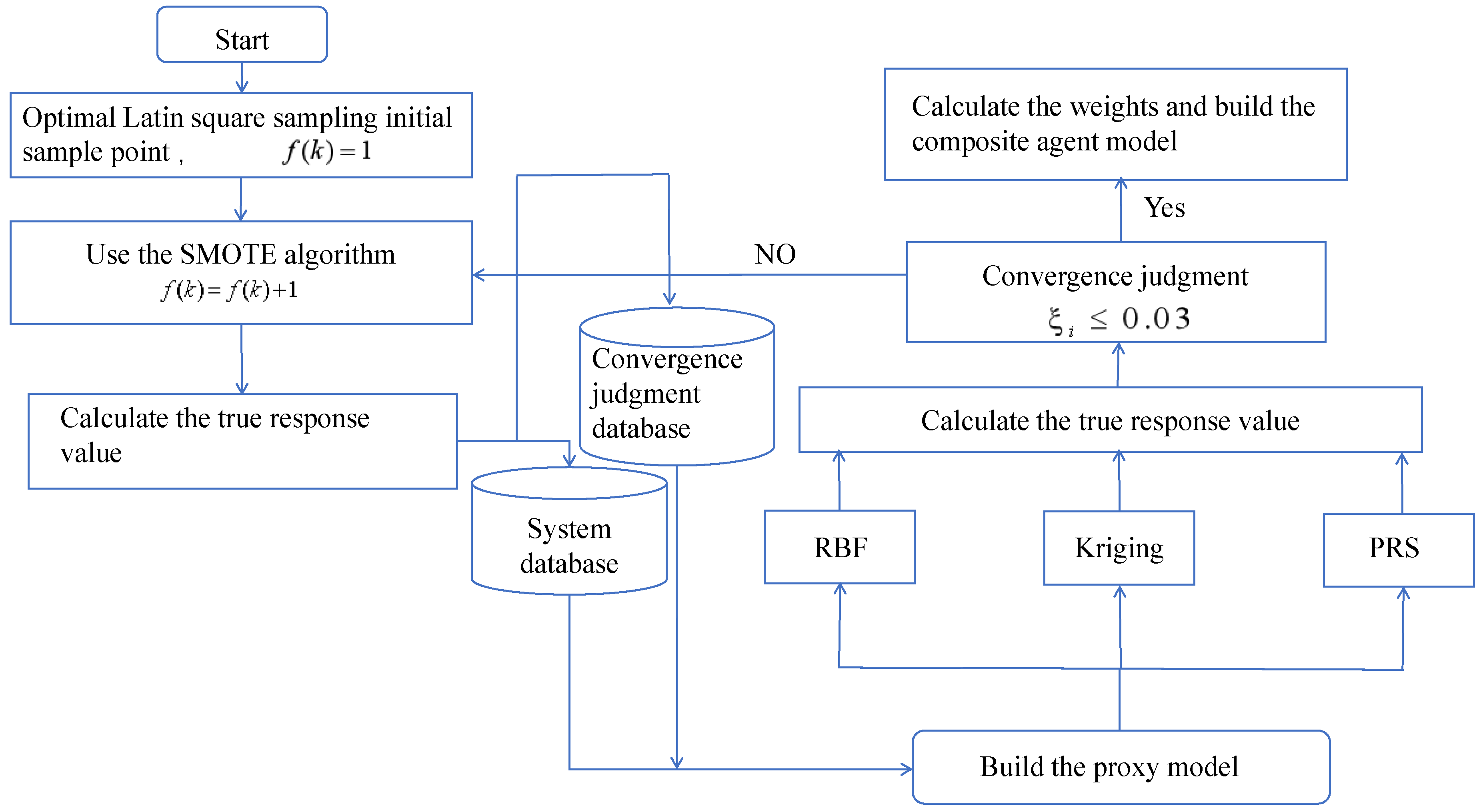
Based on the adaptive sampling method of the SMOTE algorithm and the LCB criterion, this paper applies it to the radial basis function (RBF), polynomial response surface (PRS), and Kriging model. When the three dynamic proxy models converge, the PRESS weight distribution method is used to utilize the weights to combine the three proxy models. The proxy model proposed in this paper is obtained, and the flowchart is depicted in Figure 2. The specific steps are as follows:

(1)

Utilize design of experiments (DOEs) sampling to create a real analysis model, store the resulting real response values in the database, and implement a counting function $f(k)=1$.

(2)

When $f(k)\ge 1$, call the SMOTE algorithm to interpolate the sample points in the database and obtain important sample points. Utilize orthogonal testing to determine the actual response value of these important sample points and store this information in the database.

(3)

The sample points of the database were respectively constructed with the RBF, Kriging, and PRS proxy models. The NSGA-II genetic algorithm and collaborative optimization framework are used to optimize the three proxy models, and the optimization conditions were minimized for the main subject set $f$.

(4)

To build the convergence judgment sample set, take a sample size of [10%, 20%] from the current database. Utilize the SMOTE algorithm to interpolate the dataset and acquire the actual response value through orthogonal testing. Subsequently, incorporate the constructed convergence judgment sample set into the system set for convergence judgment. The judgment conditions are as follows:

$$\frac{s(k+1)-s(k)}{s(k)}\le \xi$$

(7)

where $s(k+1)$ is the true response value after constructing a proxy model for the entire sample set and performing optimization; $s(k)$ is the true response value after optimizing the proxy model constructed by the system sample set.

(5)

Make a convergence judgment on the three proxy models individually. When the model converges, perform step (6); otherwise, return to step (2) after removing the convergence judgment sample set.

(6)

The training sample set is generated by DOEs. The predicted values are obtained using three proxy models. The training sample prediction set is saved, and the root mean square error is calculated for both the training sample set and the training sample prediction set. The root mean square error set is then retained.

(7)

The root mean square error set and weight formula (PRESS) are used to determine the weights of the three proxy models, which are then combined to create the combined proxy model.

3.2. SMOTE Algorithm

The SMOTE algorithm is an oversampling technique that balances the spatial distribution of samples by adding a small number of sample points between important sample points [19,20]. It is often used to address software defect prediction (SDP). The core idea is to (1) import the initial sample set, (2) construct important sample sets using the K-nearest neighbors algorithm (KNN), and (3) interpolate the significant sample sets to create a small number of sample sets. The flow is shown in Figure 3.

3.3. Weight Calculation

Generally, the proxy model of multimode combination has a higher generalization performance. The weight formula is typically derived from the error relationship between the actual response value and the predicted value. After measuring the error, a weight is calculated to compensate for it, thereby enhancing the fitting accuracy. The weight formula used in this paper is the PRESS formula proposed by Geol et al. [7]. The formula is as follows:

$$\overline{E}=\frac{1}{M}{\displaystyle \sum _{i=1}^M{E}_i}$$

(8)

$$E_i=\sqrt{\frac{1}{N}{\displaystyle \sum _{i=1}^M{(y_i-\overline{y_i})}^2}}$$

(9)

$$w_i^{\ast }={(E_i+\alpha \overline{E})}^{\beta }$$

(10)

$$w_i=\frac{w_i^{\ast }}{{\displaystyle \sum _{i=1}^M{E}_i}}$$

(11)

where $y_i$ is the real response value and $\overline{y_i}$ is the predicted value, $\alpha <1,\beta <0$.

For the combination of multimodal proxy models, use weight $w_i$ to weigh the predicted value $\overline{y_i}$, and finally obtain the pointwise set $y^{\ast }$ with high robust performance, as shown below.

$$y^{\ast }=w_1\overline{y_1}+w_2\overline{y_2}+w_3\overline{y_3}$$

(12)

where $w_i$ is the weight formula obtained by PRESS, $\overline{y_i}$ is the predicted value of the dynamic sampling proxy models D-RBF, D-Kriging, and D-PRS.

4. The Theoretical Foundation of Integrated Multidisciplinary Optimization Platforms

4.1. Multidisciplinary Optimization Algorithm

The traditional, non-dominated genetic algorithm is inspired by species iteration. Its computational complexity is high, making NSGA expensive for large population size calculations. Computational expensiveness results from the complexity involved in each generation of non-dominant sorting processes. Therefore, elites are introduced into each generation to enhance the convergence of the multi-objective algorithm. In this paper, NSGA-II [21] is adopted, and the optimization strategy and hierarchical analysis method are combined with the collaborative optimization framework to realize the collaborative optimization between the main system set and the subsystem set. The convergence advantage of the genetic algorithm NSGA-II is utilized to solve the multidisciplinary optimization problem of the underwater vehicle SUBOFF. For a single main discipline set function, another optimization target is to assign a minimum weight, enabling the utilization of a multi-objective optimization algorithm for a single main discipline set.

The NSGA-II principle is shown in Figure 4. First, an initial sample P_t of N numbers is generated, and then P_t is subjected to crossover and mutation to produce a new population Q_t. The new species Q_t is combined with the initial population P_t to obtain the population R_t. F1 is the optimal non-dominated solution, F2 is the suboptimal non-dominated solution, and Fn is the nth-step optimal non-dominated solution. If the number of F1 is greater than or equal to N, the members are selected from the least congested area in F1. If the number of F1 is less than N, the members in the least congested area of F2 are added. If the number is still less than N after F2 is added, the members in the least congested area of Fn are added in sequence until the number reaches N. The remaining Fn from the last generation Fs will be discarded to obtain the next generation population. This cycle is carried out for each generation.

4.2. Introduction to Proxy Models

4.2.1. Radial Basis Function (RBF) Model

An RBF neural network consists of three layers: an input layer, a hidden layer, and an output layer. Adjusting the number of sample points, hidden layer neurons, and hidden layers helps the RBF neural network enhance mapping accuracy and approximate any nonlinear function. It is classified as a feedforward neural network. Figure 5 illustrates the structure of the RBF neural network.

The radial basis function (RBF) neural network shown in Figure 5 consists of three layers: an input layer, a hidden layer, and an output layer. The input layer is directly connected to the hidden layer. The hidden layer is connected to the output layer through weighted connections.

4.2.2. Kriging Model

For an n-dimensional black-box problem, response values and parameters can be obtained through experiments. A Kriging model can be constructed using these sample points. The model function is as follows:

$$\stackrel{-}{f}(x)=p(x)+Z(x)$$

(13)

Here, $Z(x)$ represents the error term of the surrogate model. It follows a normal distribution. $p(x)$ denotes the mean of the Gaussian process in the surrogate model. The spatial function between two sample points is expressed as follows:

$${\mathrm{R}(\mathrm{x}}_i,x_j)=\exp (-{{\displaystyle \sum _{k=1}^n{\theta }_k|x_{ik}-x_{jk}|}}^{p_k})$$

(14)

Here, n denotes the n-dimensional parameters. Parameters $p(x)$ and ${\theta }_k$ are to be determined. ${\theta }_k$ controls the correlation between any two points, while $p(x)$ adjusts the smoothness of the fitted curve.

4.2.3. Polynomial Response Surface (PRS) Model

The polynomial response surface (PRS) model aims to approximate the response of complex systems using a polynomial. Usually, the PRS model is represented by a polynomial equation. This equation includes a constant term, linear terms, and interaction terms. It can be written as follows:

$$y={\mathrm{\beta }}_0+{\displaystyle \sum _{i=1}^k{\mathrm{\beta }}_i{x}_i+{\displaystyle \sum _{i=1}^k{\displaystyle \sum _{j=i}^k{\mathrm{\beta }}_{ij}{x}_i{x}_j+\dots }}}$$

(15)

In this equation, y represents the system’s response. The $x_i$(i = 0, …, k) are the input variables. The coefficient of the model is $\mathrm{\beta }$. This coefficient is typically estimated using the ordinary least squares (OLSs) method. The OLSs method works by minimizing the sum of the squared differences between the actual and predicted responses.

5. Optimization Based on a Combined Proxy Model

The underwater vehicle model SUBOFF is investigated, which originates from the Advanced Research Program project of the US Department of Defense. Since the project has published a lot of experimental data, researchers can use the published data to verify the feasibility of numerical simulation. This paper analyzes the resistance and energy consumption of the underwater vehicle SUBOFF using CFD numerical simulation.

5.1. Resistance Analysis

Computational fluid dynamics (CFD) numerical simulations provide efficient and accurate results for solving the hydrodynamic forces acting on underwater vehicles. When conducting numerical simulations, it is necessary to divide the flow field area. A flow field area that is too large will result in excessive computational costs. However, a flow field region that is too small will affect the accuracy of the numerical simulation. In this study, an analysis of the flow field region was conducted. The first half of the region was selected to be semicircular, while the second half was cylindrical, with a diameter equal to the total length of the SUBOFF, as shown in Figure 6.

When solving the Reynolds-averaged Navier–Stokes (RANS) equation, the selection of the turbulence equation is crucial. There are standard $k-\omega$, BSL $k-\omega$, GEKO $k-\omega$, SST $k-\omega$, RNG $k-\xi$, and standard $k-\xi$. In this study, the RNG $k-\xi$ equation is selected. A velocity inlet and a pressure outlet are used, with a turbulence intensity of 2 and a turbulence intensity ratio of 2%.

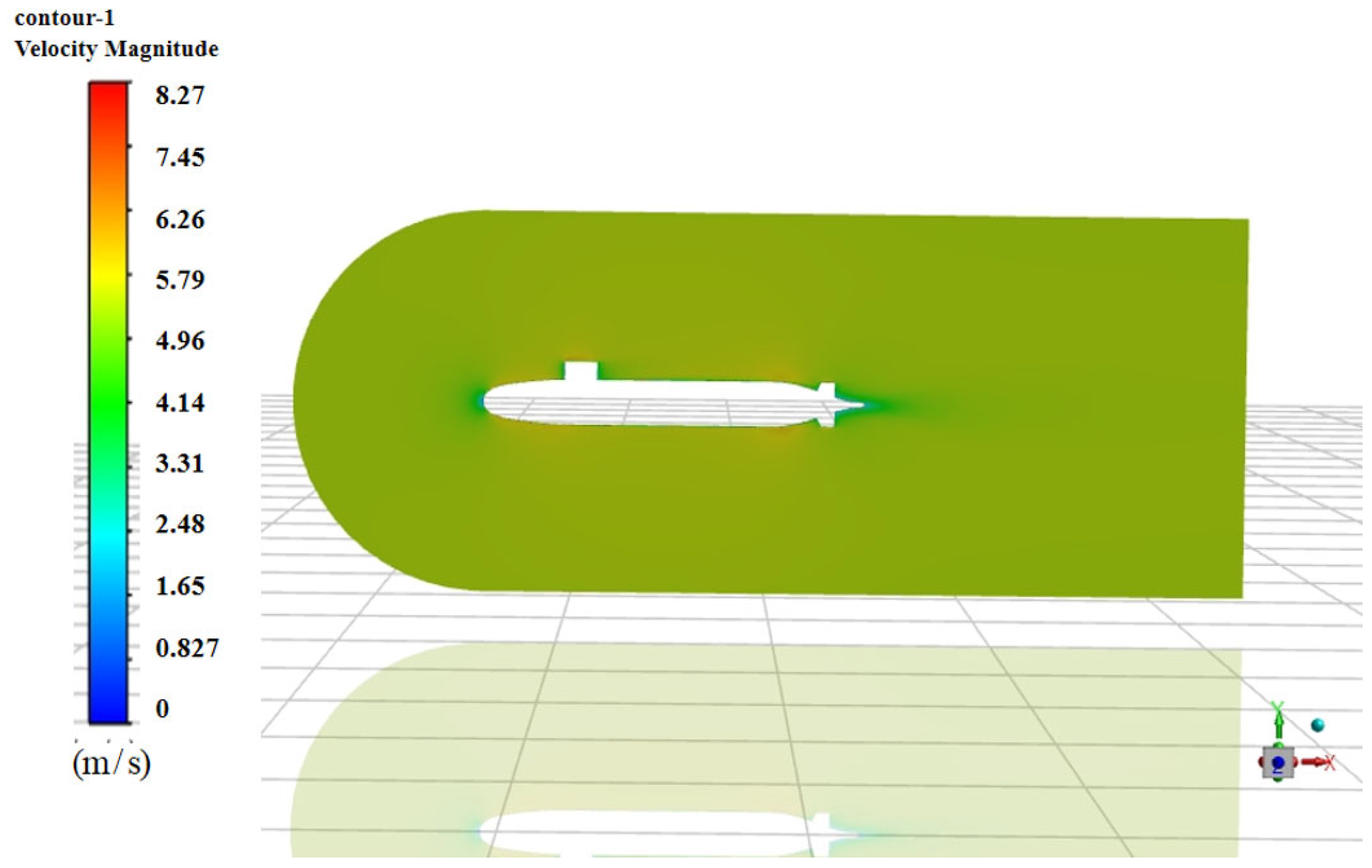
The velocity distribution around the underwater vehicle SUBFF is shown in Figure 7. The volume mesh of the SUBOFF is shown in Figure 8. The number of mesh elements is 295,085. The maximum mesh size is 0.272256 m, and the minimum mesh size is 0.01062322 m. In order to verify the correctness of numerical simulation, in this paper, the numerical simulation results are compared with the experimental data published by the U.S. Defense Program. The comparison results are shown in

Table 1. Comparison between CFD and experiment.

V (kt)	CFD (N)	Experiment (N)	Error
5.93	104	102.3	1.66%
10	279.8	283.8	1.41%
11.85	380.8	389.2	2.16%
13.92	521.8	526.6	0.91%
16	671.1	675.6	0.66%
17.79	819.9	821.1	0.15%

. As can be seen, the computational fluid dynamics (CFD) numerical simulation is accurate.

5.2. Energy Consumption Analysis

The energy consumption is related to the propulsive efficiency produced by the propeller and the resistance of the underwater vehicle. The energy consumption is calculated as follows:

$$N_e=\frac{\rho C_{d}S{v}^3}{2{\eta }_p}$$

(16)

where $\rho$ is the fluid density, $C_d$ is the drag coefficient, $S$ is the wet surface area, ${\eta }_p$ is the propulsion efficiency coefficient, and $v$ is the absolute driving speed.

The propelling efficiency of the propeller can be calculated theoretically as follows:

$${\eta }_p={\eta }_k{\eta }_l\frac{1-t}{1-E_{\mu }}$$

(17)

$${\eta }_l=1.113-0.04644\sqrt{W_K}$$

(18)

$$W_K=\frac{C_{d}S}{\pi R^2{Z}_r{(1-E_{\mu })}^2(1-t)}$$

(19)

$$E_{\mu }=E_p+E_f\frac{2+0.2\sqrt{W_K}}{1+\sqrt{1+W_K}}$$

(20)

$$u=\frac{E_{\mu }}{(1-E_{\mu })f_t}$$

(21)

$$f_u=-15.7+29.37\sqrt{W_K}-8.248W_K+23.2\lambda -39.07\sqrt{W_K}\lambda$$

(22)

The relative rotation efficiency of the propeller is denoted by ${\eta }_l$, the load coefficient is represented by $W_K$, the propeller radius is indicated by $R$, the wake efficiency is $E_{\mu }$, the number of propellers is denoted by $Z_r$, and the efficiency of the propeller in open water is ${\eta }_k$. $u$ is the thrust reduction coefficient, $f_u$ is the propeller load influence coefficient, and $\lambda$ is the pitch ratio at $r/R$ = 0.7.

5.3. Orthogonal Experimental Design

Design of experiments (DOEs) is a statistical method used to systematically design, analyze, and optimize experiments. It maximizes the utilization of data, minimizes errors, and obtains the most representative sample distribution by leveraging the orthogonal property of the design matrix within constrained experimental settings. When constructing a proxy model, it is necessary to select a sufficient and efficient number of sample points, and the design of experiments (DOEs) provides an effective method for sample collection. To enhance sampling efficiency and ensure the quality of space filling, this paper opts for the optimal Latin method for sample collection.

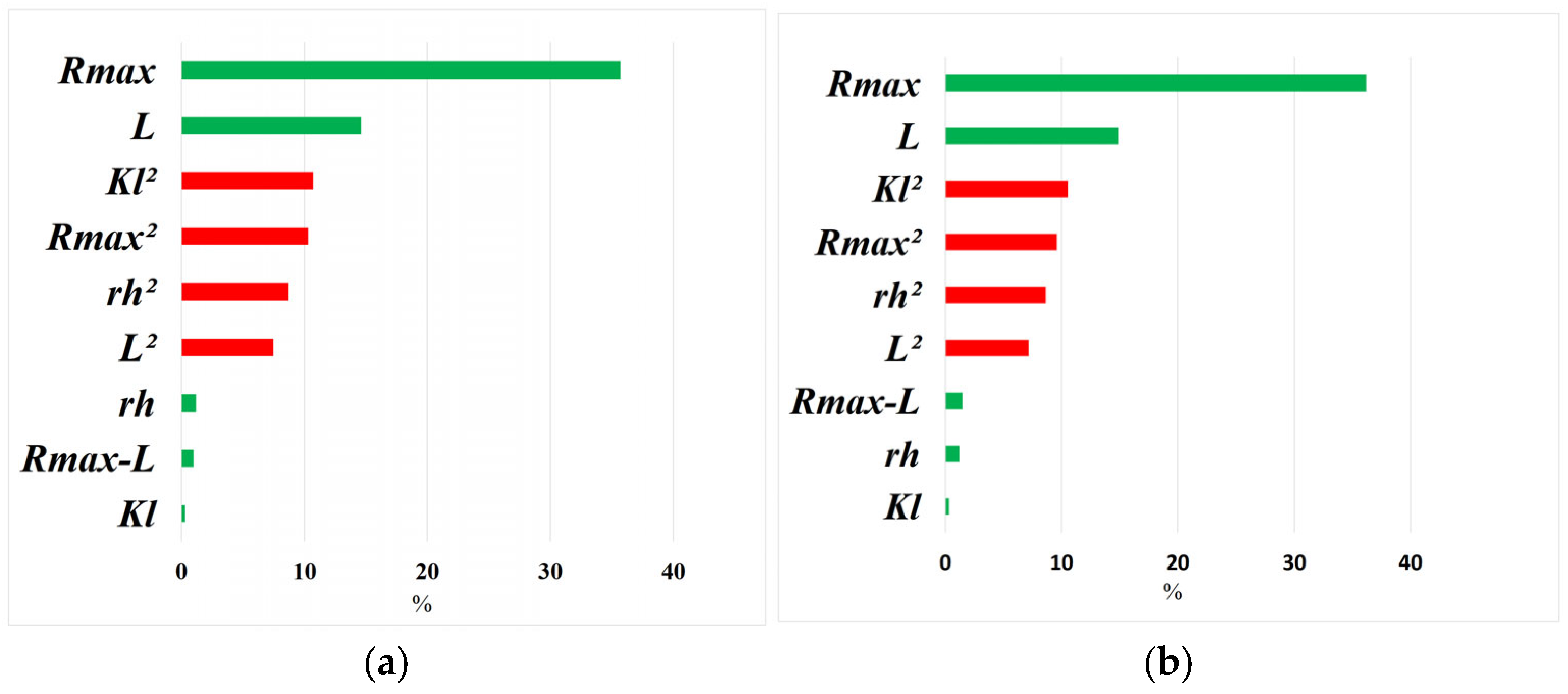
To design the test parameters effectively, it is necessary to obtain important parameters. Therefore, a sensitivity analysis of the parameters is conducted. Through this method, the most effective parameter variable can be selected to reduce the number of design parameters and enhance test efficiency. The parameters examined in this paper include the minimum radius of the afterbody $rh$, the smoothness index of the tail $Kl$, the maximum radius $R_{\max }$, and the length of the parallel midbody $L$. Sensitivity analysis on the resistance and energy consumption of the SUBOFF is conducted. The green bar indicates a positive correlation, while the red bar indicates a negative correlation, as shown in Figure 9.

5.4. Multidisciplinary Optimization Framework

Based on the collaborative optimization framework, the coupling relationship between the main subject level and the sub-subject level is considered. Based on the hierarchical analysis method, the primary subject-level function is obtained as follows:

$$f=0.6813Fd+0.3187Ne$$

(23)

where $Fd$ is the resistance and $Ne$ is the energy consumption.

Based on the sensitivity analysis in Figure 8, the sub-discipline function is designed. In the field of rapidity discipline, the main focus is on the influence of resistance on the underwater vehicle. The design parameters include linear terms $R_{\max }$, $L$, and $rh$. The design function is shown as follows:

$$f_1={(R_{\max 1}-R_{\max })}^2+{(L_1-L)}^2+{(r{h}_1-rh)}^2$$

(24)

For the energy consumption discipline, it can be obtained from the analysis in Figure 8 that the linear terms $R_{\max }$, $L$, and cross term $\left(R_{\max }-L\right)$ are selected as the design variables, and the design function is shown as follows:

$$f_2={(R_{\max 2}-R_{\max })}^2+{(R_{\max 2}-L_2-R_{\max }+L)}^2+{(L_2-L)}^2$$

(25)

5.5. Proxy Model Convergence Condition

When the error between the optimal value and the true response value is less than or equal to 2% and the convergence factor is $\epsilon \le 0.03$, the model achieves convergence. The convergence verification uses 10% to 20% of the total database sample set to construct the convergence judgment sample set. The convergence judgment sample set is constructed using the SMOTE algorithm and the orthogonal experimental design. The convergence judgment sample set is added to the total database sample set for convergence judgment.

The process of convergence judgment is shown in Figure 10. First, at the Kth optimization, the proxy model is constructed using the total sample set. Subsequently, the proxy models RBF, PRS, and Kriging are constructed, and the real response values are calculated. Then, the convergence judgment sample set is added to the total sample set. Subsequently, at the (K + 1)th optimization, the proxy models RBF, PRS, and Kriging are constructed. Using the Kth and (K + 1)th actual response values to calculate the convergence factor for the three proxy models, respectively. When the convergence factors of the three proxy models are $\epsilon \le 0.03$, the model converges.

5.6. Optimization Results

In this paper, the NSGA-II genetic algorithm and collaborative optimization framework are utilized for the multi-objective optimization of underwater vehicles. The optimization stopping criterion is defined as follows: the optimization process halts when the difference between the current optimal value and the previous optimal value is less than 0.001, i.e., ${|F}_{op}-F\left(k\right)|<0.001$. In addition, three dynamic proxy models (D-RBF, D-Kriging, D-PRS) and three static proxy models (S-RBF, S-Kriging, S-PRS) were used to analyze the error relationship between the predicted value and the actual response value during optimization. The analysis also included the number of calls made to the real model by both the static and dynamic proxy models, as presented in

Table 2. Comparison of model calling times and the accuracy of different proxy models.

Model	Number of Model Calls	Resistance	Energy Consumption
D-PRS	70	1.158%	1.135%
D-Kriging	70	0.145%	0.104%
D-RBF	70	0.095%	0.119%
S-PRS	97	1.753%	2.02%
S-Kriging	97	0.54%	0.61%
S-RBF	97	0.314%	0.330%

.

It can be seen from Table 2 that after dynamically processing the sampling points, the optimization efficiency of the underwater vehicle is improved, and the dynamic proxy model exhibits high fitting accuracy.

As shown in Table 2, the dynamic proxy model has a higher fitting accuracy than the static proxy model. To validate that the proposed combined proxy model (CPM) has high fitting accuracy, a comparison between the CPM and the three dynamic proxy models is sufficient. This comparison is illustrated in Figure 11.

The results of the SUBOFF optimization based on the model are shown in

Table 3. Performance comparison before and after the SUBOFF optimization.

	Initial Value	Optimal Value
Fd (N)	292.27	270.9 (−7.312%)
Ne (N·m/s)	1291.21	1184.75 (−8.245%)

. It can be seen that the resistance and energy consumption of the SUBOFF are significantly reduced, improving the rapid performance of the SUBOFF and saving energy.

The root mean square error (RMSE) and mean absolute percentage error (MAPE) of the combined proxy model (CPM) and three dynamic proxy models (D-RBF, D-Kriging, and D-PRS) are shown in Figure 11. It can be seen that the root mean square error (RMSE) and mean absolute percentage error (MAPE) of the combined proxy model (CPM) are the lowest, indicating high fitting accuracy. For various types of engineering problems, the proxy model demonstrates good generalization performance. For example, Figure 12 shows the comparison between CPM and other models when a reducer [22] optimization is investigated. As can be seen, among the models to be compared, the D-RBF model performs the best instead of the D-Kriging model, as shown in Figure 11. Nevertheless, the proposed CPM also achieves better generalization performance. Generally, the proxy model has high generalization performance and high accuracy in fitting.

Figure 13 and Figure 14 show the profile plot of an underwater vehicle before and after optimization. In Figure 12, the black line represents the before optimization, while the red line represents the after optimization. It can be observed that in the underwater vehicle, the length of the profile is shorter, the radius of the midship body is reduced, and the fatness of the tail profile is increased.

6. Conclusions

In this study, a multidisciplinary optimization design of an underwater vehicle was conducted using a collaborative optimization framework and the NSGA-II genetic algorithm. A proxy model and optimization platform were established based on the SMOTE algorithm and weight allocation. The following conclusions can be drawn from the optimization results:

(1)

After comparing the combined proxy model built based on the SMOTE algorithm and weight allocation method with other dynamic agent models, it can be seen that it demonstrates good fitting accuracy, optimization efficiency, and generalization performance.

(2)

The optimization strategy based on a collaborative optimization framework and the NSGA-II genetic algorithm is applied to the underwater vehicle SUBOFF, demonstrating high efficiency and convergence in optimization.

(3)

The optimization strategy is applied to the underwater vehicle SUBOFF. According to the optimization results, the fast performance and energy-saving capabilities of the underwater vehicle SUBOFF have also been enhanced.

This study did not use a large number of low-dimensional to high-dimensional functions to validate the performance of the combined proxy model. Proxy models often perform poorly with high-dimensional functions. This study primarily focuses on calculations for the underwater vehicle engineering example and does not analyze the performance of particularly high-dimensional issues. Future research will address high-dimensional problems. For engineering problems, considering only speed and energy consumption is insufficient. The maneuverability, energy consumption, stealth, and lightweight design of underwater vehicles must also be considered. Additionally, the analysis of low-speed underwater vehicles is inadequate, and the wave resistance at high speeds needs to be considered.

References

1. Long, T.; Guo, X.; Peng, L.; Liu, L. Optimization strategy using dynamic radial basis function metamodel based on trust region. J. Mech. Eng. 2014, 50, 184–190. (In Chinese) [Google Scholar] [CrossRef]
2. Long, T.; Li, X.; Huang, B.; Jiang, M. Aerodynamic and stealthy performance optimization of airfoil based on adaptive surrogate model. J. Mech. Eng. 2016, 52, 101–111. (In Chinese) [Google Scholar] [CrossRef]
3. Diez Silvia, M.; Andrea, V.; Stern, F. Simulation-based design optimization by sequential multi-criterion adaptive sampling and dynamic radial basis functions. In Proceedings of the 11th International Conference on Evolutionary and Deterministic Methods for Design, Optimization and Control with Applications to Industrial and Societal Problems, Glasgow, UK, 14–16 September 2015; pp. 213–228. [Google Scholar]
4. Su, G.; Peng, L.; Hu, L. A Gaussian process-based dynamic surrogate model for complex engineering structural reliability analysis. Struct. Saf. 2017, 68, 97–109. [Google Scholar] [CrossRef]
5. Luo, W.; Guo, X.; Dai, J.; Rao, T. Hull optimization of an underwater vehicle based on dynamic proxy model. Ocean. Eng. 2021, 230, 109050. [Google Scholar] [CrossRef]
6. Pan, W.; Luo, W. Lines optimisation of an underwater vehicle using SMOTE and adaptive minimise LCB based dynamic proxy models. Ships Offshore Struct. 2024, 19, 91–108. [Google Scholar] [CrossRef]
7. Goel, T.; Haftka, R.T.; Shyy, W.; Queipo, N.V. Ensemble of surrogates. Struct. Multidiscip. Optim. 2007, 33, 199–216. [Google Scholar] [CrossRef]
8. Lee, Y.; Choi, D.H. Pointwise ensemble of meta-models using v nearest points cross-validation. Struct. Multidiscip. Optim. 2014, 50, 383–394. [Google Scholar] [CrossRef]
9. Chen, H.; Li, W.; Cui, W.; Liu, Q. A pointwise ensemble of surrogates with adaptive function and heuristic formulation. Struct. Multidiscip. Optim. 2022, 65, 113. [Google Scholar] [CrossRef]
10. Yang, X.; Guo, T.; Yu, M.; Chen, M. Optimization of engineering parameters of deflagration fracturing in shale reservoirs based on hybrid proxy model. Geoenergy Sci. Eng. 2023, 231, 212318. [Google Scholar] [CrossRef]
11. Zhang, D.; Song, B.; Wang, P.; Chen, X. Multidisciplinary optimization design of a new underwater vehicle with highly efficient gradient calculation. Struct. Multidiscip. Optim. 2017, 55, 1483–1502. [Google Scholar] [CrossRef]
12. Mohsen, B.; Mehdi, M.; Mehdi, S. A new approach in system and tactic design optimization of an autonomous underwater vehicle by using Multidisciplinary Design Optimization. Ocean. Eng. 2018, 147, 517–530. [Google Scholar]
13. Chen, X.; Wang, P.; Zhang, D. Surrogate-based Multidisciplinary Design Optimization of an Autonomous Underwater Vehicle Hull. In Proceedings of the 2017 16th International Symposium on Distributed Computing and Applications to Business, Engineering and Science(DCABES 2017), Anyang, China, 13–16 October 2017. [Google Scholar]
14. Lyu, W.; Luo, W. Design of underwater robot lines based on a hybrid automatic optimization strategy. J. Mar. Sci. Appl. 2014, 13, 274–280. [Google Scholar] [CrossRef]
15. Liu, X.; Yuan, Q.; Zhao, M.; Cui, W.; Ge, T. Multiple objective multidisciplinary design optimization of heavier-than-water underwater vehicle using CFD and approximation model. J. Mar. Sci. Technol. 2017, 22, 135–148. [Google Scholar] [CrossRef]
16. Adelman, H.M.; Mantay, W.R. Integrated multidisciplinary design optimization of rotorcraft. J. Aircr. 1991, 28, 22–28. [Google Scholar] [CrossRef]
17. Kroo, I.; Altus, S.; Braun, R.; Gage, P.; Sobieski, I. Multidisciplinary Optimization Methods for Aircraft Preliminary Design. In Proceedings of the 5th Symposium on Multidisciplinary Analysis and Optimization, Panama City Beach, FL, USA, 7–9 September 1994; pp. 697–707. [Google Scholar]
18. Sobieszczanski-Sobieski, J.; Agte, J.S.; Sandusky, R.R. Bilevel integrated system synthesis. AIAA J. 2000, 38, 164–172. [Google Scholar] [CrossRef]
19. Nitesh, V.C.; Kevin, W.B.; Lawrence, O.H. SMOTE: Synthetic Minority Over-sampling Technique. J. Artif. Intell. Res. 2002, 16, 321–357. [Google Scholar]
20. Pak, C.; Wang, T.T.; Su, X.H. An empirical study on software defect prediction using over-sampling by SMOTE. Int. J. Softw. Eng. Knowl. Eng. 2018, 28, 811–830. [Google Scholar] [CrossRef]
21. Deb, K.; Pratap, A.; Agarwal, S.; Meyarivan, T.A.M.T. A fast and elitist multiobjective genetic algorithm: NSGA-II. IEEE Trans. Evol. Comput. 2002, 6, 182–197. [Google Scholar] [CrossRef]
22. Kodiyalam, S. Evaluation of Methods for Multidisciplinary Design Optimization (MDO), Phase I; National Aeronautics and Space Administration, Langley Research Center: Hampton, VA, USA, 1998. [Google Scholar]
Figure 1. Collaborative optimization framework.
Jmse 12 01087 g001
Figure 2. Combined proxy model construction.
Jmse 12 01087 g002
Figure 3. SMOTE algorithm.
Jmse 12 01087 g003
Figure 4. NSGA-II scheme.
Jmse 12 01087 g004
Figure 5. Structure of the RBF neural network.
Jmse 12 01087 g005
Figure 6. Flow field area of the SUBOFF.
Jmse 12 01087 g006
Figure 7. Velocity distribution around the SUBOFF.
Jmse 12 01087 g007
Figure 8. Volume mesh of the SUBOFF.
Jmse 12 01087 g008
Figure 9. Parameter sensitivity analysis: (a) resistance; (b) energy consumption.
Jmse 12 01087 g009
Figure 10. Convergence judgment.
Jmse 12 01087 g010
Figure 11. Error comparison between agent models in optimizing the SUBOFF model: (a) MAPE of resistance; (b) RMSE of resistance; (c) MAPE of energy consumption; (d) RMSE of energy consumption.
Jmse 12 01087 g011
Figure 12. Error comparison between proxy models in optimizing a reducer: (a) RSME; (b) MAPE.
Jmse 12 01087 g012
Figure 13. Comparison of optimized front and rear lines: (a) before optimization; (b) after optimization.
Jmse 12 01087 g013
Figure 14. Comparison of the geometric model of the SUBOFF before and after optimization.
Jmse 12 01087 g014