A Joint Graph-Based Approach for Simultaneous Underwater Localization and Mapping for AUV Navigation Fusing Bathymetric and Magnetic-Beacon-Observation Data

Abstract

Accurate positioning is the necessary basis for autonomous underwater vehicles (AUV) to perform safe navigation in underwater tasks, such as port environment monitoring, target search, and seabed exploration. The position estimates of underwater navigation systems usually suffer from an error accumulation problem, which makes the AUVs difficult use to perform long-term and accurate underwater tasks. Underwater simultaneous localization and mapping (SLAM) approaches based on multibeam-bathymetric data have attracted much attention for being able to obtain error-bounded position estimates. Two problems limit the use of multibeam bathymetric SLAM in many scenarios. The first is that the loop closures only occur in the AUV path intersection areas. The second is that the data association is prone to failure in areas with gentle topographic changes. To overcome these problems, a joint graph-based underwater SLAM approach that fuses bathymetric and magnetic-beacon measurements is proposed in this paper. In the front-end, a robust dual-stage bathymetric data-association method is used to first detect loop closures on the multibeam bathymetric data. Then, a magnetic-beacon-detection method using Euler-deconvolution and optimization algorithms is designed to localize the magnetic beacons using a magnetic measurement sequence on the path. The loop closures obtained from both bathymetric and magnetic-beacon observations are fused to build a joint-factor graph. In the back-end, a diagnosis method is introduced to identify the potential false factors in the graph, thus improving the robustness of the joint SLAM system to outliers in the measurement data. Experiments based on field bathymetric datasets are performed to test the performance of the proposed approach. Compared with classic bathymetric SLAM algorithms, the proposed algorithm can improve the data-association accuracy by 50%, and the average positioning error after optimization converges to less than 10 m.

1. Introduction

The underwater navigation system is critical in order for underwater vehicles to perform activities that require long-duration and accurate positioning [1,2]. Given the absence of Global Navigation Satellite System (GNSS) signals underwater, the principal navigation systems predominantly rely on the Inertial Navigation System (INS), complemented by Doppler Velocity Log (DVL), underwater acoustic transponders, and geophysical field data [3,4]. The INS provides autonomous position estimation but is susceptible to error accumulation due to its integral solution method. DVL can help to reduce the INS accumulated error greatly, but the navigation output still contains approximate linear-growth errors. Acoustic positioning systems, such as long baseline, short baseline, and ultra-short baseline systems, offer precise positions within their working ranges. Nonetheless, their deployment necessitates intricate advance preparation and is quite costly and time-consuming.

Geophysical field-aided navigation methods have garnered significant interest for enhancing the reliability of underwater navigation systems [5,6,7]. In areas where prior geophysical field maps are available, the positioning errors can be bounded through data-matching approaches. Conversely, in unknown environments, a Simultaneous Localization and Mapping (SLAM) approach is usually taken to correct the accumulated errors through data association based on the measured data in real time. Several studies involving the utilization of bathymetric data for underwater navigation have been conducted to evaluate practical performance. The Norwegian Defense Research Establishment has carried out a series of simulations and experimental works on terrain-matching algorithms using the HUGIN AUV [8,9,10]. Stanford University and the Monterey Bay Aquarium Research Institute collaborated on the development of a long-range and low-cost AUV terrain navigation system [11,12]. By using low-precision dead-reckoning (DR) and filtering algorithms, a positioning accuracy of 4–10 m is achieved. Roman C and Singh H proposed an improved SLAM approach for multibeam seafloor mapping [13,14]. To create more accurate topographic maps, the multibeam-sonar data is divided into submaps that are used for registration. Meanwhile, the delayed state extended Kalman filter (EKF) is used to re-navigate vehicle trajectories.

The research into geomagnetic field-aided navigation methods for marine vehicles has garnered significant attention. Huang et al. proposed a method for long-range navigation of underwater autonomous underwater vehicles using magnetic anomalies generated by magnetic dipoles [15]. In their study, the magnetic-gradient tensor and the draft depth are used to achieve continuous underwater positioning. The relative positioning error is less than 4% on average in simulation experiments. Alimi et al. demonstrated the viability of using passive magnets for underwater navigation, estimating the position of the sensor with a relative error of 1% to 3% through real-world systematic studies [16]. Chang et al. proposed a magnetic beacon-based simultaneous localization and mapping (SLAM) approach [17,18]. This approach based on particle filter is designed to correct the vehicle-position errors by identifying magnetic beacons in unknown background magnetic fields. Du et al. devised a program to track a mobile-magnetic-dipole target and estimated its magnetic moments using measurements from multiple scalar magnetometers. This program enables rapid detection of the direction, velocity, elevation angle, and magnetic moment of the target [19]. Wu and Yao proposed an adaptive SLAM-based method for magnetic-gradient-aided navigation [20]. The magnetic-gradient values of landmarks are measured by magnetometers that are installed on an underwater vehicle. Subsequently, an adaptive-unscented-Kalman filter-SLAM method is applied to derive optimal estimations of the vehicle poses.

In underwater SLAM systems, the AUVs detect the seabed using sonar or cameras. The images or bathymetric data obtained are then used to make data associations for positioning-error correction [21,22]. The main steps include the following: (1) accurate environmental-data observation; (2) effective data association; and (3) robust state estimation. Magnetic SLAM is mainly based on the magnetic-dipole model, and in order to establish the observation equation, the measurements used are usually magnetic-field intensity or magnetic-field gradient. Lee et al. used the gradient-based magnetic tensor to identify and locate ferromagnetic objects in the environment. Two different types of dense objects are used to verify the effectiveness and accuracy of a proposed method [23]. In bathymetric SLAM, the multibeam echo sonar (MBES) method is used to collect bathymetric data in pings, and the iterative closest point (ICP) method is commonly employed for data association. Palomer et al. used MBES to collect three-dimensional bathymetric point clouds and used heuristic ICP to eliminate the influence of point cloud uncertainty on registration accuracy [24,25]. Jung et al. proposed a regularized ICP method by re-scaling bathymetric values to improve the data-association accuracy in areas with poor topographic features [26]. Bichucher et al. proposed an xy-alignment generalized ICP (GICP) algorithm to create registration between bathymetric submaps [27]. This proposed algorithm aims to enforce consistent bathymetric structures and constrain long-term navigation drift.

The SLAM solutions can be broadly categorized into filter-based and graph-based methods. Filtering methods primarily comprise extended Kalman filter (EKF) and particle filter (PF) methods [28,29]. For instance, Callmer et al. presented a silent underwater SLAM scheme employing triaxial magnetometers as sensors to locate a vessel with a known magnetic dipole, with trajectory and sensor positions estimated simultaneously using an extended Kalman filter (EKF) [30]. Torroba et al. proposed a Rao-Blackwellized particle filter (RBPF) SLAM solution for online large-scale SLAM in an embedded platform, incorporating implicit data association for terrain-loop closure detection and utilizing the particle filter to fuse terrain constraints and estimate AUV poses [31]. Additionally, He et al. integrated the particle swarm optimization (PSO) method into Fast SLAM to enhance AUV pose estimation accuracy, adapting PSO to optimize particles and prevent particle degeneracy and impoverishment [32]. The filtering methods often have a high computational complexity when the state vector is of high dimension, and their accuracy can be easily affected by unstable measurement noises. The graph-based SLAM approach utilizes factor graphs to represent the relationships between nodes in the SLAM system, where vehicle poses and observed objects are represented as nodes and odometry and loop closures are represented as edges. The optimization of trajectories and maps is achieved using a cost function composed of the edges in the factor graph [33]. Graph optimization methods have been applied in BSLAM and magnetic-beacon SLAM studies. Ling et al. used a sparse pseudo-input Gauss process (SPGP) to establish weak data association between adjacent moments and used a terrain-matching method to obtain closed loops among survey moments, and the underwater vehicle positions were estimated using a graph optimization method [34]. In order to solve the effect of invalid loop closures on SLAM results, some robust algorithms have been proposed. Sunderhauf and Protzel added switch variables to the objective function to obtain a robust solution for pose graph SLAM. The switch variables can enable or disable the factors associated with them [35]. Latif et al. proposed a realizing, reversing, and recovering (RRR) algorithm based on the consensus that correct loop closures tend to agree among themselves and agree with the sequential constraints from odometry, to create robust loop closures in SLAM [36].

This paper proposes a joint graph-based underwater SLAM approach that fuses bathymetric and magnetic beacon measurements. In the front-end, magnetic beacon observations and bathymetric loop closures are generated based on the Euler-deconvolution method and the dual-stage-data-association method, respectively; in the back-end, the generated constraints in the front-end are used to construct the factor graph, and a robust optimizer is used to estimate the AUV path and construct a bathymetric map. The main contributions are as follows:

• A novel dual-stage bathymetric data-association method is introduced. The curvature feature vectors on different scales are used to make robust transformations in the first stage, and the GICP algorithm is taken to make fine registrations in the second stage.
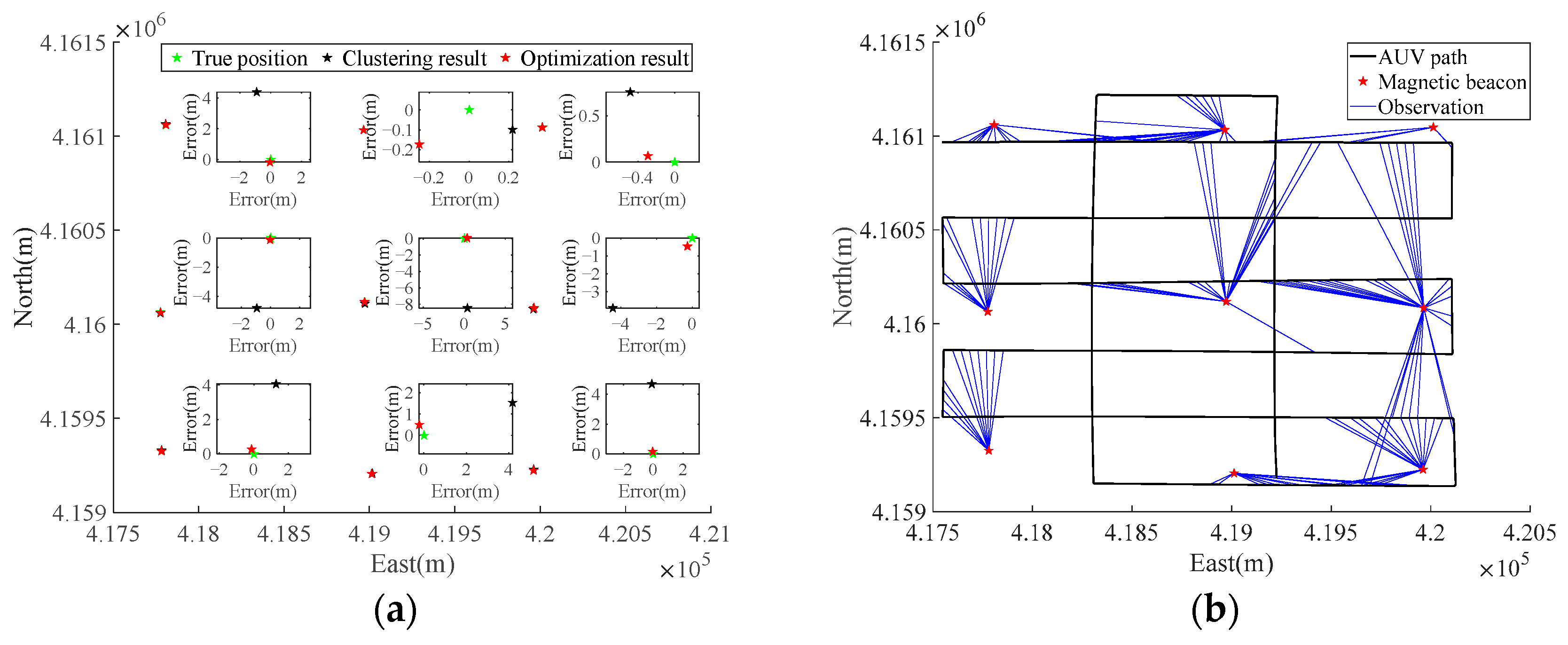
• Magnetic beacons are used to aid bathymetric data to give better SLAM performance. Also, a new approach that combines Euler-deconvolution and clustering methods is presented that can be used to locate the magnetic beacons accurately in real time.
• A false loop-closure-factor-diagnosis mechanism that considers positioning uncertainty, heading, and bathymetric consistency is designed and introduced to the novel back-end optimizer. The robustness of the SLAM system to bad data-association results is subsequently improved.

The remaining sections of the paper are organized as below. The robust dual-stage multibeam-bathymetric-point-cloud-registration method is introduced in Section 2, followed by the magnetic-beacon-detection approach introduced in Section 3. The back-end graph optimizer with a false loop-closure-diagnosis-mechanism design is introduced in Section 4. Last of all, experiments and analysis are given in Section 5.

2. Dual-Stage Bathymetric Registration Using Curvature-Based Method and GICP

There are usually some outliers in the multibeam bathymetric dataset. To perform bathymetric SLAM in real time, a denoising method is introduced first in this section. At the same time, to improve the data-association accuracy using bathymetric point clouds, the Gaussian-process-regression method is used to model and resample the topographic data. On the basis of this, a dual-stage bathymetric registration approach is presented to make data associations between bathymetric point clouds.

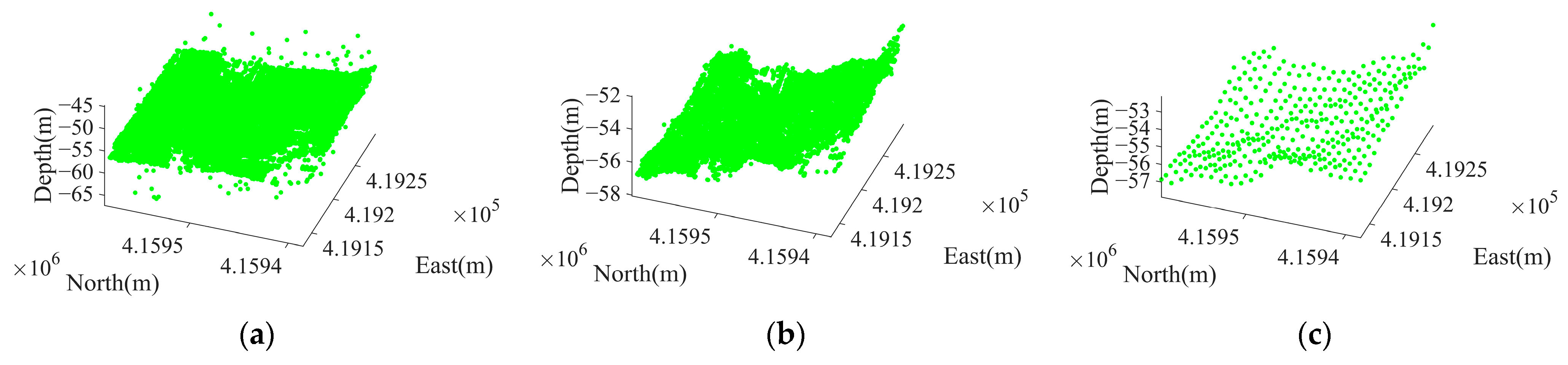
2.1. Denoising and Down-Sampling of Multibeam-Bathymetric Data

2.1.1. Denoising of Bathymetric Point Clouds

A statistical method is used to remove the outliers from the bathymetric point cloud by detecting the bathymetric difference among neighbor points. For each bathymetric point in the cloud, the mean $u$ and standard deviation $\sigma$ of the K-nearest neighbors is calculated. If a bathymetric point differs from $u$ by greater than 3$\sigma$, then it will be taken as an outlier. Specific steps are as follows:

(1) Read the bathymetric point cloud $\mathrm{S}=\{{\mathbf{b}}_i,i=\mathrm{1,2},\dots ,n\}$;

(2) Use the k-dimensional tree to index the bathymetric points in the cloud to speed up the searching efficiency for the closest points.

(3) Search the K-nearest neighbors for each bathymetric point ${\mathbf{b}}_i\in \mathrm{S}$ and put them in a set $\mathrm{N}\mathrm{b}\left({\mathbf{b}}_i\right)$.

(4) Calculate the bathymetric difference ${\mathrm{D}}_{\mathrm{mid}}$ between ${\mathbf{b}}_i$ and the mean value of $\mathrm{N}\mathrm{b}\left({\mathbf{b}}_i\right)$ as in Equation (1).

$${\mathrm{D}}_{\mathrm{mid}}\left({\mathbf{b}}_i\right)=\left|{\mathbf{b}}_{i,\mathrm{z}}-\frac{1}{\mathrm{K}}{\displaystyle \sum _{{\mathbf{b}}_k\in \mathrm{N}\mathrm{b}\left({\mathbf{b}}_i\right)}}{\mathbf{b}}_{k,\mathrm{z}}\right|$$

(1)

If ${\mathrm{D}}_{\mathrm{mid}}\left({\mathbf{b}}_i\right)>3\sigma$, then ${\mathbf{b}}_i$ will be taken as an outlier and removed. Otherwise, it will be retained.

(5) Repeat steps (3) and (4) for all bathymetric points in the cloud.

2.1.2. Bathymetric Down-Sampling Using Gaussian Process Regression

The purpose of bathymetric down-sampling is to reduce the density of the points without reducing the matching suitability. Gaussian process regression (GPR) is a non-parametric model that uses Gaussian process priors to perform regression analysis [37]. Assuming that the bathymetric points obey the multidimensional Gaussian distribution, the GPR can achieve high-precision and uniform down-sampling on the bathymetric point cloud. Let ${\mathrm{z}}_i$ indicate the bathymetric value of the point ${\mathbf{x}}_i=\{{\mathbf{b}}_{i,\mathrm{x}},{\mathbf{b}}_{i,\mathrm{y}}\}$. The fitted function between ${\mathbf{x}}_i$ and ${\mathrm{z}}_i$ can be expressed as Equation (2).

$${\mathrm{z}}_i=\mathrm{f}\left({\mathbf{x}}_i\right)+\mathcal{N}\left(0,{\sigma }_{\mathrm{n}}^2\right)$$

(2)

where $\mathrm{f}\left(\mathbf{x}\right)=\mathrm{G}\mathrm{P}\left(\mathrm{m}\left(\mathbf{x}\right),\mathrm{k}\left(\mathbf{x},\mathbf{x}\prime \right)\right)$ is the Gaussian process with known mean and variance, and ${\sigma }_{\mathrm{n}}^2$ is the variance of measurement noise. $\mathrm{k}\left(\mathbf{x},\mathbf{x}\prime \right)$ is the kernel function that computes the covariance between two bathymetric points $\mathbf{x}$ and $\mathbf{x}\prime$ as,

$$\mathrm{k}\left(\mathbf{x},\mathbf{x}\prime \right)={\sigma }_{\mathrm{f}}^2\exp \left[\frac{-{\left(\mathbf{x}-\mathbf{x}\prime \right)}^2}{2l^2}\right]+{\sigma }_{\mathrm{n}}^2\mathsf{\delta }\left(\mathbf{x},\mathbf{x}\prime \right)$$

(3)

where the first term on the right side represents the square exponential covariance kernel function, and the second term represents the Kronecker delta function. The $l$, ${\sigma }_{\mathrm{f}}$, and ${\sigma }_{\mathrm{n}}$ values are the hyperparameters of the kernel function.

Using the disordered bathymetric point cloud as the training set to find the optimal hyperparameters, the coordinate ${\mathbf{x}}^{\ast }$ of an interpolation point is input into the model, and the depths ${\mathrm{z}}^{\ast }$ can be estimated.

The joint distribution of the training data z and estimated value ${\mathrm{z}}^{\ast }$ is expressed as

$$\left[\begin{array}{c}z\\ {\mathrm{z}}^{\ast }\end{array}\right]~\mathcal{N}\left(0,\left[\begin{array}{cc}\mathrm{k}\left(\mathbf{x},\mathbf{x}\right)& {\mathrm{k}\left({\mathbf{x}}^{\ast },\mathbf{x}\right)}^{\mathrm{\top }}\\ \mathrm{k}\left({\mathbf{x}}^{\ast },\mathbf{x}\right)& \mathrm{k}\left({\mathbf{x}}^{\ast },{\mathbf{x}}^{\ast }\right)\end{array}\right]\right)=\mathcal{N}\left(0,\left[\begin{array}{cc}\mathbf{C}& {\mathbf{C}}_{\ast }^{\mathrm{\top }}\\ {\mathbf{C}}_{\ast }& {\mathbf{C}}_{\ast \ast }\end{array}\right]\right)$$

(4)

where $\mathbf{C}$ is the covariance matrix of training data $\mathbf{x}$, ${\mathbf{C}}_{\ast }$ is the covariance matrix between the train data $\mathbf{x}$ and the interpolation points ${\mathbf{x}}^{\ast }$, and ${\mathbf{C}}_{\ast \ast }$ is the covariance matrix of ${\mathbf{x}}^{\ast }$. The ${\mathrm{z}}^{\ast }$ can then be estimated as shown in Equation (5),

$$\mathrm{p}\left({\mathrm{z}}^{\ast }\left|{\mathbf{x}}^{\ast }\right.\right)=\mathcal{N}\left(\mathrm{m}\left({\mathrm{z}}^{\ast }\right),\mathrm{cov}\left({\mathrm{z}}^{\ast }\right)\right)$$

(5)

In which

$$\mathrm{m}\left({\mathrm{z}}^{\ast }\right)={\mathbf{C}}_{\ast }{\mathbf{C}}^{-1}\mathrm{z}$$

(6)

$$\mathrm{cov}\left({\mathrm{z}}^{\ast }\right)={\mathbf{C}}_{\ast \ast }-{\mathbf{C}}_{\ast }{\mathbf{C}}^{-1}{\mathbf{C}}_{\ast }^{\mathrm{\top }}$$

(7)

An example of the denoising and down-sampling of a multibeam bathymetric dataset is shown in Figure 1.

2.2. Dual-Stage Bathymetric Data Association

The initial position of two bathymetric point clouds strongly affects the iterative closest point (ICP) results [38], especially for bathymetric maps with low overlap ratio and low matching suitability. To achieve accurate data association, a rough registration method based on feature vectors is proposed in the first stage. Then, in the second stage, the generalized ICP (GICP) is used to obtain accurate loop closure. The detailed process is shown in Algorithm 1.

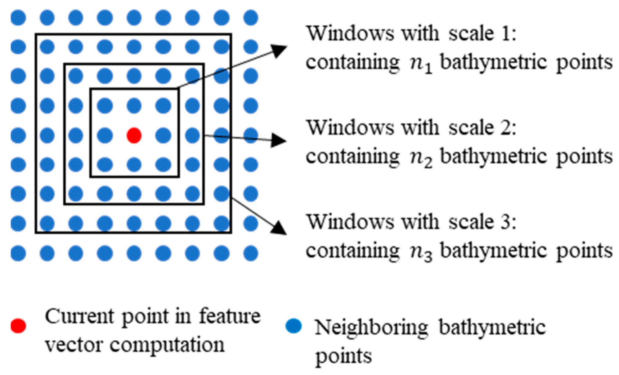
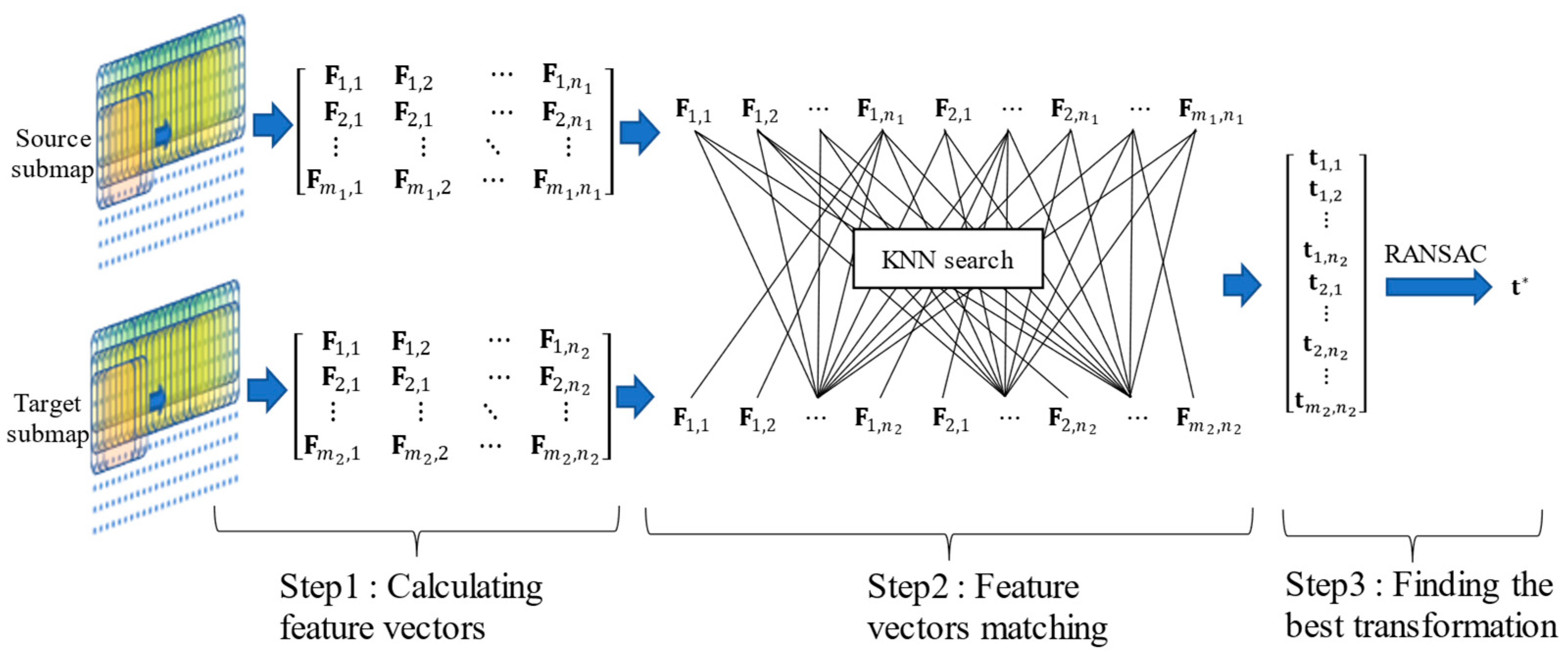
2.2.1. Coarse Registration Based on Multi-Scale Feature Vectors

A curvature is selected to represent the topographic change between adjacent bathymetric points. First, the multi-scale curvature feature vectors are established for the points. For each point, the k-nearest neighbor points form a surface $\mathrm{S}:\mathrm{z}=\mathrm{z}(\mathrm{x},\mathrm{y})$. With a definition $\overrightarrow{\mathbf{r}}\triangleq \left\{\mathrm{x},\mathrm{y},\mathrm{z}\left(\mathrm{x},\mathrm{y}\right)\right\}$, the first-order and second-order partial derivative of $\overrightarrow{\mathbf{r}}$ with respect to $x$ and $y$ can be calculated as ${\overrightarrow{\mathbf{r}}}_{\mathrm{x}}=\left\{\mathrm{1,0},\partial \mathrm{z}/\partial \mathrm{x}\right\}$, ${\overrightarrow{\mathbf{r}}}_{\mathrm{y}}=\left\{\mathrm{1,0},\partial \mathrm{z}/\partial \mathrm{y}\right\}$, ${\overrightarrow{\mathbf{r}}}_{\mathrm{x}\mathrm{x}}=\left(\mathrm{0,0},{\partial }^2\mathrm{z}/{\partial \mathrm{x}}^2\right)$, ${\overrightarrow{\mathbf{r}}}_{\mathrm{x}\mathrm{y}}=\left(\mathrm{0,0},{\partial }^2\mathrm{z}/\partial \mathrm{x}\partial \mathrm{y}\right)$, ${\overrightarrow{\mathbf{r}}}_{\mathrm{y}\mathrm{y}}=\left(\mathrm{0,0},{\partial }^2\mathrm{z}/{\partial \mathrm{y}}^2\right)$. The unit vector of the principal normal to the surface is

$$\overrightarrow{\mathbf{n}}=\frac{\left({\overrightarrow{\mathbf{r}}}_{\mathrm{x}}\times {\overrightarrow{\mathbf{r}}}_{\mathrm{y}}\right)}{\left|{\overrightarrow{\mathbf{r}}}_{\mathrm{x}}\cdot {\overrightarrow{\mathbf{r}}}_{\mathrm{y}}\right|}$$

(8)

Denoted by $E={\overrightarrow{\mathbf{r}}}_{\mathrm{x}}\cdot {\overrightarrow{\mathbf{r}}}_{\mathrm{x}}, F={\overrightarrow{\mathbf{r}}}_{\mathrm{x}}\cdot {\overrightarrow{\mathbf{r}}}_{\mathrm{y}},G={\overrightarrow{\mathbf{r}}}_{\mathrm{y}}\cdot {\overrightarrow{\mathbf{r}}}_{\mathrm{y}}$, $L={\overrightarrow{\mathbf{r}}}_{\mathrm{x}\mathrm{x}}\cdot \overrightarrow{\mathbf{n}},M={\overrightarrow{\mathbf{r}}}_{\mathrm{x}\mathrm{y}}\cdot \overrightarrow{\mathbf{n}}$, and $N={\overrightarrow{\mathbf{r}}}_{\mathrm{y}\mathrm{y}}\cdot \overrightarrow{\mathbf{n}}$, the average curvature $H$ and Gaussian curvature $K$ of surface $\mathrm{S}$ can be calculated by Equations (9) and (10), respectively.

$$H=\frac{EG+GL-2FM}{2\left(EG-F^2\right)}=k_1\cdot k_2$$

(9)

$$K=\frac{LN-M^2}{EG-F^2}=\frac{1}{2}\left(k_1+k_2\right)$$

(10)

where $k_1$ and $k_2$ are the maximum and minimum curvatures of the surface S, also called the principal curvature. They can be calculated using Equations (11) and (12), respectively.

$$k_1=H+\sqrt{H^2-K}$$

(11)

$$k_2=H-\sqrt{H^2-K}$$

(12)

Then, the Gaussian curvature, mean curvature, and principal curvature form a feature vector $\mathbf{c}$ as

$$\mathbf{c}=[H,K,k_1,k_2]$$

(13)

With each bathymetric point as a center, three different-scale square windows are created that contain $n_1$, $n_2$, and $n_3$ bathymetric points, respectively, as shown in Figure 2. The feature vector $\mathbf{F}$ is formed as Equation (14).

$$\mathbf{F}=\left[{\mathbf{c}}_{n_1},{\mathbf{c}}_{n_2},{\mathbf{c}}_{n_3}\right]$$

(14)

where ${\mathbf{c}}_{n_i}$ can be computed using Equation (13). $n_1$, $n_2$, and $n_3$ are set to 9, 16, and 25 in this research, respectively. The cosine similarity is used to evaluate the similarity of two bathymetric point clouds, as shown in Equation (15)

$$\mathrm{S}\left({\mathbf{F}}^{\mathrm{P}},{\mathbf{F}}^{\mathrm{Q}}\right)=\frac{{\mathbf{F}}^{\mathrm{P}}\cdot {\mathbf{F}}^{\mathrm{Q}}}{‖{\mathbf{F}}^{\mathrm{P}}‖\times ‖{\mathbf{F}}^{\mathrm{Q}}‖}=\frac{{\sum }_{i=1}^n\left({\mathbf{F}}_i^{\mathrm{P}}\times {\mathbf{F}}_i^{\mathrm{Q}}\right)}{\sqrt{{\sum }_{i=1}^n{{\mathbf{F}}_i^{\mathrm{P}}}^2}\times \sqrt{{\sum }_{i=1}^n{{\mathbf{F}}_i^{\mathrm{Q}}}^2}}$$

(15)

P and Q are used to indicate the source and target bathymetric point clouds, respectively. $n$ is the number of bathymetric points in a cloud. $\mathrm{S}\left({\mathbf{F}}^{\mathrm{P}},{\mathbf{F}}^{\mathrm{Q}}\right)$ is the cosine value of the angle between two n-dimensional vectors. The Random Sample Consensus (RANSAC) algorithm [39] is used to select the best transformation between the two clouds. Specific steps are given as follows:

(1)

Randomly select a translation ${\mathbf{t}}_i$ between two matched points, between which the curvature feature vectors have the highest similarity.

(2)

Use ${\mathbf{t}}_i$ to transform the source point clouds P.

(3)

Find the closest point pairs in between Q and P, and count the number of point pairs with bathymetric differences less than the consistency threshold $\tau$.

(4)

Repeat steps (1)–(3) until enough iterations are performed. Then, the translation ${\mathbf{t}}^{\ast }$ with the largest $n$ is selected as the final transformation.

This method is illustrated in Figure 3.

2.2.2. Fine Registration Based on GICP

Generalized ICP (GICP) is an extension of the traditional ICP algorithm. GICP improves the distance metric of the ICP algorithm with a probability model and is more suitable for dealing with noisy point cloud registration problems [40].

Base on the coarse registration result, the closest point pairs between the source point cloud $\mathrm{P}={\left\{{\mathbf{b}}_i^{\mathrm{P}}\right\}}_{i=1,\dots ,N}$ and target point cloud $\mathrm{Q}={\left\{{\mathbf{b}}_i^{\mathrm{Q}}\right\}}_{i=1,\dots ,N}$ can be determined as an initialization for the fine registration.

The transformation between $\mathrm{P}$ and $\mathrm{Q}$ can be established as in Equation (16).

$${\mathbf{b}}_i^{\mathrm{P}}=\mathbf{R}·{\mathbf{b}}_i^{\mathrm{Q}}+\mathbf{t}=\left(\begin{array}{cc}\mathbf{R}& \mathbf{t}\\ 0& 1\end{array}\right)·{\mathbf{b}}_i^{\mathrm{Q}}=\mathbf{T}·{\mathbf{b}}_i^{\mathrm{Q}}$$

(16)

The bathymetric values of the source points and target points are supposed to obey Gaussian distribution, as ${\mathbf{b}}_i^{\mathrm{P}}\sim \mathcal{N}\left({\widehat{\mathbf{b}}}_i^{\mathrm{P}},{\mathbf{C}}_i^{\mathrm{P}}\right),{\mathbf{b}}_i^{\mathrm{Q}}\sim \mathcal{N}\left({\widehat{\mathbf{b}}}_i^{\mathrm{Q}},{\mathbf{C}}_i^{\mathrm{Q}}\right)$. Denoting the true transformation by ${\mathbf{b}}_i^{\mathrm{P}}={\mathbf{T}}^{\ast }·{\mathbf{b}}_i^{\mathrm{Q}}$, the transformation error of $\mathbf{T}$ can be calculated as in Equation (17), and the probabilistic distribution can be represented as in Equation (18).

$${\mathrm{d}}_i^{\left(\mathbf{T}\right)}={\mathbf{b}}_i^{\mathrm{P}}-\mathbf{T}·{\mathbf{b}}_i^{\mathrm{Q}}$$

(17)

$${\mathrm{d}}_i^{\left(\mathbf{T}\right)}=\mathcal{N}\left({\widehat{\mathbf{b}}}_i^{\mathrm{Q}}-{\mathbf{T}}^{\ast }{\widehat{\mathbf{b}}}_i^{\mathrm{Q}},{\mathbf{C}}_i^{\mathrm{Q}}+\left({\mathbf{T}}^{\ast }\right){\mathbf{C}}_i^{\mathrm{P}}{\left({\mathbf{T}}^{\ast }\right)}^{\mathrm{\top }}\right)=\mathcal{N}\left(0,{\mathbf{C}}_i^{\mathrm{Q}}+\left({\mathbf{T}}^{\ast }\right){\mathbf{C}}_i^{\mathrm{P}}{\left({\mathbf{T}}^{\ast }\right)}^{\mathrm{\top }}\right)$$

(18)

The optimal transformation is obtained by minimizing the transformation error. The $\mathbf{T}$ can be calculated using maximum likelihood estimation

$$\mathbf{T}={\displaystyle \underset{\mathbf{T}}{\mathrm{a}\mathrm{r}\mathrm{g}\mathrm{m}\mathrm{a}\mathrm{x}}}\prod _i\mathrm{p}\left({\mathrm{d}}_i^{\left(\mathbf{T}\right)}\right)={\displaystyle \underset{\mathbf{T}}{\mathrm{a}\mathrm{r}\mathrm{g}\mathrm{m}\mathrm{a}\mathrm{x}}}\prod _i\log \left(\mathrm{p}\left({\mathrm{d}}_i^{\left(\mathbf{T}\right)}\right)\right)={\displaystyle \underset{\mathbf{T}}{\mathrm{a}\mathrm{r}\mathrm{g}\mathrm{m}\mathrm{i}\mathrm{n}}}\sum _i{\left({\mathrm{d}}_i^{\left(\mathbf{T}\right)}\right)}^{\mathrm{\top }}{\left({\mathbf{C}}_i^{\mathrm{Q}}+\left({\mathbf{T}}^{\ast }\right){\mathbf{C}}_i^{\mathrm{P}}{\left({\mathbf{T}}^{\ast }\right)}^{\mathrm{\top }}\right)}^{-1}{\mathrm{d}}_i^{\left(\mathbf{T}\right)}$$

(19)

The complete dual-stage bathymetric data-association approach is summarized in Algorithm 1 below.

Algorithm 1: Bathymetric point cloud registration

Input: Source bathymetric submap $\mathrm{P}$, target bathymetric submap $\mathrm{Q}$ Output: Transformation $[{\mathbf{R}}^{\ast },{\mathbf{t}}^{\ast \ast }]$ Step1: Denoising and down-sampling   $\mathrm{P},\mathrm{Q}=\mathrm{p}\mathrm{r}\mathrm{e}\mathrm{p}\mathrm{r}\mathrm{o}\mathrm{c}\mathrm{e}\mathrm{s}\mathrm{s}(\mathrm{P},\mathrm{Q})$ Step2: Establishing curvature feature vectors   ${\mathbf{c}}^{\mathrm{P}},{\mathbf{c}}^{\mathrm{Q}}=\mathrm{c}\mathrm{u}\mathrm{r}\mathrm{v}\mathrm{a}\mathrm{t}\mathrm{u}\mathrm{r}\mathrm{e}\left(\mathrm{P},\mathrm{Q}\right)$   ${\mathbf{F}}^{\mathrm{P}}=\left[{\mathbf{c}}_{\mathrm{s}\mathrm{c}\mathrm{a}\mathrm{l}\mathrm{e}1}^{\mathrm{P}},{\mathbf{c}}_{\mathrm{s}\mathrm{c}\mathrm{a}\mathrm{l}\mathrm{e}2}^{\mathrm{P}},{\mathbf{c}}_{\mathrm{s}\mathrm{c}\mathrm{a}\mathrm{l}\mathrm{e}3}^{\mathrm{P}}\right]$, ${\mathbf{F}}^{\mathrm{Q}}=\left[{\mathbf{c}}_{\mathrm{s}\mathrm{c}\mathrm{a}\mathrm{l}\mathrm{e}1}^{\mathrm{Q}},{\mathbf{c}}_{\mathrm{s}\mathrm{c}\mathrm{a}\mathrm{l}\mathrm{e}2}^{\mathrm{Q}},{\mathbf{c}}_{\mathrm{s}\mathrm{c}\mathrm{a}\mathrm{l}\mathrm{e}3}^{\mathrm{Q}}\right]$ Step3: Computing the similarity use cosine distance, and using KNN algorithm to select the best match   $\mathrm{i}\mathrm{n}\mathrm{d}\mathrm{e}\mathrm{x}=\mathrm{K}\mathrm{N}\mathrm{N}\mathrm{s}\mathrm{e}\mathrm{a}\mathrm{r}\mathrm{c}\mathrm{h}({\mathbf{F}}^{\mathrm{P}},{\mathbf{F}}^{\mathrm{Q}},\prime \mathrm{c}\mathrm{o}\mathrm{s}\mathrm{i}\mathrm{n}\mathrm{e}\prime )$ Step4: Selecting the best transform with RANSAC   $\mathbf{t}={\mathbf{F}}^{\mathrm{P}}\left(\mathrm{i}\mathrm{n}\mathrm{d}\mathrm{e}\mathrm{x}\right)-{\mathbf{F}}^{\mathrm{Q}}$   ${\mathbf{t}}^{\ast }=\mathrm{R}\mathrm{A}\mathrm{N}\mathrm{S}\mathrm{A}\mathrm{C}(\mathrm{P},\mathrm{Q},\mathbf{t})$   ${\mathbf{F}}^{\mathrm{P}\ast }={\mathbf{F}}^{\mathrm{P}}-{\mathbf{t}}^{\ast }$ Step5: Using GICP for fine registration $[{\mathbf{R}}^{\ast },{\mathbf{t}}^{\ast \ast }]=\mathrm{G}\mathrm{I}\mathrm{C}\mathrm{P}({\mathbf{F}}^{\mathbf{P}\ast },{\mathbf{F}}^{\mathbf{Q}})$

3. Detection of Magnetic Beacons

To use the magnetic beacons as landmarks to obtain more loop closures in SLAM, an accurate detection method is essential in order to obtain relative localizations of the beacons. A new magnetic-beacon-detection method is proposed in this paper. First, the Euler-deconvolution method is utilized to obtain the general location of potential beacons near the AUV track. Second, the Euler-deconvolution results are taken as initializations for the nonlinear optimization approach, which is used to obtain the accurate positions of the beacons simultaneously. The detailed process is given in Algorithm 2.

Algorithm 2: Optimization of magnetic-beacon positions

Input: AUV pose $\mathbf{x}=\left\{{\mathbf{x}}_1,{\mathbf{x}}_2,\dots ,{\mathbf{x}}_n\right\}$, Magnetometer observation $\mathbf{B}=\left\{{\mathbf{B}}_1,{\mathbf{B}}_2,\dots ,{\mathbf{B}}_n\right\}$ Output: Magnetic beacon location $\mathbf{m}$=$\left\{{\mathbf{m}}_1,{\mathbf{m}}_2,\dots ,{\mathbf{m}}_m\right\}$, Observation $\mathbf{z}$ Step1: Calculating magnetic-field gradient, and setting observations interval are taken as $k$   $\mathbf{G}=\mathrm{g}\mathrm{r}\mathrm{a}\mathrm{d}\mathrm{i}\mathrm{e}\mathrm{n}\mathrm{t}\left(\mathbf{B}\right)$   for $i=1:k:n-k$     ${\mathbf{x}}_i^{\mathrm{s}\mathrm{e}\mathrm{g}}=\left\{{\mathbf{x}}_{i+1},{\mathbf{x}}_{i+2},\dots ,{\mathbf{x}}_{i+k}\right\}$     ${\mathbf{B}}_i^{\mathrm{s}\mathrm{e}\mathrm{g}}=\left\{{\mathbf{B}}_{i+1},{\mathbf{B}}_{i+2},\dots ,{\mathbf{B}}_{i+k}\right\}$     ${\mathbf{G}}_i^{\mathrm{s}\mathrm{e}\mathrm{g}}=\left\{{\mathbf{G}}_{i+1},{\mathbf{G}}_{i+2},\dots ,{\mathbf{G}}_{i+k}\right\}$ Step2: Locating the relative positions of the magnetic beacons and clustering the locations of magnetic beacons   for $j=1:k$     ${\mathbf{r}}_j=-3{{\mathbf{G}}_j^{\mathrm{s}\mathrm{e}\mathrm{g}}}^{-1}\left({\mathbf{B}}_j^{\mathrm{s}\mathrm{e}\mathrm{g}}-{\mathbf{B}}^{\mathrm{e}}\right)$     ${\mathbf{m}}_{ini}=\mathrm{D}\mathrm{B}\mathrm{S}\mathrm{C}\mathrm{A}\mathrm{N}\left({\mathbf{x}}_j^{seg}+{\mathbf{r}}_j\right)$   end Step3: Multi-objective joint optimization   $e^{\mathrm{B}}={\left[{\mathbf{B}}_i^{\mathrm{s}\mathrm{e}\mathrm{g}}-\mathrm{b}\left({\mathbf{m}}_{ini}\right)-{\mathbf{B}}_{\mathbf{b}}\right]{\mathsf{\Omega }}_{\mathrm{B}}^{-1}\left[{\mathbf{B}}_i^{\mathrm{s}\mathrm{e}\mathrm{g}}-\mathrm{b}\left({\mathbf{m}}_{ini}\right)-{\mathbf{B}}_{\mathbf{b}}\right]}^{\mathrm{\top }}$   $e^{\mathrm{G}}=\left[{\mathbf{G}}_i^{\mathrm{s}\mathrm{e}\mathrm{g}}-\mathrm{g}\left({\mathbf{m}}_{ini}\right)\right]{\mathsf{\Omega }}_{\mathrm{G}}^{-1}{\left[{\mathbf{G}}_i^{\mathrm{s}\mathrm{e}\mathrm{g}}-\mathrm{g}\left({\mathbf{m}}_{ini}\right)\right]}^{\mathrm{\top }}$   ${\mathbf{m}}_{\mathrm{o}\mathrm{p}\mathrm{t}}^{\ast }={\displaystyle \underset{{\mathbf{m}}_{\mathit{ini}}}{\mathrm{argmin}}}\left(e^{\mathrm{B}}+e^{\mathrm{G}}\right)$ Step4: Updating the set of magnetic beacons and logging magnetic-beacon observations   for ${\mathbf{m}}_k^{\ast }$ in ${\mathbf{m}}_{\mathrm{o}\mathrm{p}\mathrm{t}}^{\ast }$     if ${\mathbf{m}}_k^{\ast }$ not in $\mathrm{M}$       $\mathbf{m}=\{\mathbf{m},{\mathbf{m}}_k^{\ast }\}$     end     $\mathbf{z}$=[$\mathbf{z}$;$i,k,{\mathbf{x}}_i^{\mathrm{s}\mathrm{e}\mathrm{g}}-{\mathbf{m}}_k^{\ast }(1:3)$]   end end

3.1. Fast Identification Using Euler-Deconvolution and Clustering Methods

As the distances between the vehicle and magnetic beacons deployed on seabed are much larger than the beacon size, the beacons can be treated as magnetic dipoles [41]. Placing the magnetic beacon on the coordinate origin, the magnetic field it generates at point $\mathrm{P}\left(x,y,z\right)$ can be simplified as Equation (20)

$$\left[\begin{array}{c}{B}_{\mathbf{x}}\\ B_{\mathbf{y}}\\ B_{\mathbf{z}}\end{array}\right]=\frac{\mu }{4\pi r^5}\left[\begin{array}{ccc}3x^2-{‖\mathit{r}‖}^2& 3xy& 3xz\\ 3xy& 3y^2-{‖\mathit{r}‖}^2& 3yz\\ 3zx& 3yz& 3z^2-{‖\mathit{r}‖}^2\end{array}\right]\left[\begin{array}{c}{m}_{\mathbf{x}}\\ m_{\mathbf{y}}\\ m_{\mathbf{z}}\end{array}\right]$$

(20)

where $B_{\mathbf{x}}$, $B_{\mathbf{y}}$ and $B_{\mathbf{z}}$ are magnetic-field component of the beacons in the x, y and z directions, respectively. $\mu$ is the permeability of the medium, and ${\mu }_0=4\mathsf{\pi }\times {10}^{-7}\mathrm{V}·\mathrm{s}/(\mathrm{A}·\mathrm{m})$ in vacuum. $\mathbf{r}$ is the vector from the beacon to point P, and $‖\mathbf{r}‖=\sqrt{x^2+y^2+z^2}$.

The magnetic-gradient tensor $\mathbf{G}$ describes the changes of $B_{\mathbf{x}}$, $B_{\mathbf{y}}$, and $B_{\mathbf{z}}$ in the x, y and z directions, as shown in Equation (21).

$$\mathbf{G}=\left[\begin{array}{ccc}\frac{\partial B_{\mathbf{x}}}{\partial x}& \frac{\partial B_{\mathbf{y}}}{\partial x}& \frac{\partial B_{\mathbf{z}}}{\partial x}\\ \frac{\partial B_{\mathbf{x}}}{\partial y}& \frac{\partial B_{\mathbf{y}}}{\partial y}& \frac{\partial B_{\mathbf{z}}}{\partial y}\\ \frac{\partial B_{\mathbf{x}}}{\partial z}& \frac{\partial B_{\mathbf{y}}}{\partial z}& \frac{\partial B_{\mathbf{z}}}{\partial z}\end{array}\right]\triangleq \left[\begin{array}{ccc}{g}_{\mathrm{x}\mathrm{x}}& g_{\mathrm{y}\mathrm{x}}& g_{\mathrm{z}\mathrm{x}}\\ g_{\mathrm{x}\mathrm{y}}& g_{\mathrm{y}\mathrm{y}}& g_{\mathrm{z}\mathrm{y}}\\ g_{\mathrm{x}\mathrm{z}}& g_{\mathrm{y}\mathrm{z}}& g_{\mathrm{z}\mathrm{z}}\end{array}\right]$$

(21)

When the AUV navigates in the magnetic-beacon deployment area, the magnetic strength and gradient it measures are the sum of the magnetic fields of the Earth the and beacons, as shown in Equations (22) and (23).

$$\mathbf{B}\triangleq {\left[\begin{array}{ccc}{B}_{\mathbf{x}}& B_{\mathbf{y}}& B_{\mathbf{z}}\end{array}\right]}^{\mathrm{T}}={\left[\begin{array}{ccc}{B}_{\mathrm{x}}^{\mathrm{b}}& B_{\mathrm{y}}^{\mathrm{b}}& B_{\mathrm{z}}^{\mathrm{b}}\end{array}\right]}^{\mathrm{T}}+{\left[\begin{array}{ccc}{B}_{\mathrm{x}}^{\mathrm{e}}& B_{\mathrm{y}}^{\mathrm{e}}& B_{\mathrm{z}}^{\mathrm{e}}\end{array}\right]}^{\mathrm{T}}$$

(22)

$$\mathbf{G}\triangleq {\left[\begin{array}{ccc}{\mathbf{G}}_{\mathbf{x}}& {\mathbf{G}}_{\mathbf{y}}& {\mathbf{G}}_{\mathbf{z}}\end{array}\right]}^{\mathrm{T}}={\mathbf{G}}^{\mathrm{b}}+{\mathbf{G}}^{\mathrm{e}}$$

(23)

where the superscripts b and e indicate the beacon and Earth, respectively. The ${\mathbf{B}}^{\mathrm{e}}\triangleq {\left[\begin{array}{ccc}{B}_{\mathrm{x}}^{\mathrm{e}}& B_{\mathrm{y}}^{\mathrm{e}}& B_{\mathrm{z}}^{\mathrm{e}}\end{array}\right]}^{\mathrm{T}}$ can be computed from global or local magnetic models accurately. Due to the weak spatial change of the Earth’s magnetic field, ${\mathbf{G}}^{\mathrm{e}}$ is much smaller than ${\mathbf{G}}^{\mathrm{b}}$ and thus can be neglected.

The tensor Euler-deconvolution (TED) method [42] can be used by AUVs to estimate the position of the magnetic sources. The magnetic anomaly field satisfies the homogeneous Euler equations

$$x\frac{\partial \mathbf{B}}{\partial x}+y\frac{\partial \mathbf{B}}{\partial y}+z\frac{\partial \mathbf{B}}{\partial z}=-n\left(\mathbf{B}-{\mathbf{B}}^{\mathrm{e}}\right)$$

(24)

where $n$ is the structure index of the source. For magnetic-dipole sources, $n$ = 3. Then, we obtain

$$\mathbf{r}=-3{\mathbf{G}}^{-1}\left(\mathbf{B}-{\mathbf{B}}^{\mathrm{e}}\right)$$

(25)

Furthermore, to improve the robustness of TED against measurement noise in source localization, the Eigen analysis of the magnetic-gradient tensor (EGT) is used together with TED to improve the location accuracy. As $\mathbf{G}$ is a real symmetrical matrix, the eigenvector set $\left\{{\mathbf{b}}_1,{\mathbf{b}}_2,{\mathbf{b}}_3\right\}$ of $\mathbf{G}$ can be obtained. The ${\mathbf{b}}_3$ corresponds to the smallest eigenvalue and is perpendicular to the plane $\mathbf{m}-\mathbf{r}$, in which $\mathbf{m}$ is the magnetic moment vector of the beacon. This means that the $\mathbf{r}$ to be solved is orthogonal to ${\mathbf{b}}_3$. Let ${\mathbf{b}}_3={\left[\begin{array}{ccc}{b}_{3\mathrm{x}}& b_{3\mathrm{y}}& b_{3\mathrm{z}}\end{array}\right]}^{\mathrm{T}}$ and $\mathbf{r}={\left[\begin{array}{ccc}{r}_{\mathrm{x}}& r_{\mathrm{y}}& r_{\mathrm{z}}\end{array}\right]}^{\mathrm{T}}$, then

$$b_{3\mathrm{x}}·r_{\mathrm{x}}+b_{3\mathrm{y}}·r_{\mathrm{y}}+b_{3\mathrm{z}}·r_{\mathrm{z}}=0$$

(26)

Then, we obtain Equation (27) by combining Equations (25) and (26). Compared with Equation (25), the solution space of $\mathbf{r}$ is significantly reduced and can be solved with the least square method.

$$\left[\begin{array}{ccc}{g}_{\mathrm{x}\mathrm{x}}& g_{\mathrm{y}\mathrm{x}}& g_{\mathrm{z}\mathrm{x}}\\ g_{\mathrm{x}\mathrm{y}}& g_{\mathrm{y}\mathrm{y}}& g_{\mathrm{z}\mathrm{y}}\\ g_{\mathrm{x}\mathrm{z}}& g_{\mathrm{y}\mathrm{z}}& g_{\mathrm{z}\mathrm{z}}\\ b_{3\mathrm{x}}& b_{3\mathrm{y}}& b_{3\mathrm{z}}\end{array}\right]\left[\begin{array}{c}{r}_{\mathrm{x}}\\ r_{\mathrm{y}}\\ r_{\mathrm{z}}\end{array}\right]=-3\left[\begin{array}{c}{B}_{\mathrm{x}}^{\mathrm{b}}\\ B_{\mathrm{y}}^{\mathrm{b}}\\ B_{\mathrm{z}}^{\mathrm{b}}\\ 0\end{array}\right]$$

(27)

The measurement noise also affects the TED+EGT performance greatly. With an increase in distance between the vehicle and magnetic beacons, the influence of measurement noise on inversion results increases. For each beacon, the inversion results obtained from the vehicle positions close to it show obvious convergence, whereas those obtained from far vehicle positions contain large errors and differ from each other greatly. We use the Density-Based Spatial Clustering of Applications with Noise (DBSCAN) [43] method to cluster the estimated locations of the beacons.

Supposing there are $n$ beacon locations $\mathcal{R}$= {${\mathbf{r}}_1$,${\mathbf{r}}_2$,…,${\mathbf{r}}_n$}, the distance between ${\mathbf{r}}_i$ and ${\mathbf{r}}_j$ can be computed as

$$\mathrm{D}\mathrm{i}\mathrm{s}\mathrm{t}\left({\mathbf{r}}_i,{\mathbf{r}}_j\right)=\sqrt{{\left(r_{i,\mathrm{x}}-r_{j,\mathrm{x}}\right)}^2+{\left(r_{i,\mathrm{y}}-r_{j,\mathrm{y}}\right)}^2+{\left(r_{i,\mathrm{z}}-r_{j,\mathrm{z}}\right)}^2}$$

(28)

For a location ${\mathbf{r}}_i$, the points in $\mathcal{R}$ that are shorter than $\epsilon$ from the location form a set $\mathcal{N}\left({\mathbf{r}}_i\right)$, as in Equation (29)

$$\mathcal{N}\left({\mathbf{r}}_i\right)=\left\{{\mathbf{r}}_j\in \mathcal{R}|\mathrm{D}\mathrm{i}\mathrm{s}\mathrm{t}\left({\mathbf{r}}_i,{\mathbf{r}}_j\right)\le \epsilon \right\}$$

(29)

If the number of elements in $\mathcal{N}\left({\mathbf{r}}_i\right)$ is larger than a given threshold, then ${\mathbf{r}}_i$ will be taken as a core point and a new cluster $\mathcal{N}\left({\mathbf{r}}_i\right)$ is formed. Then, each element in $\mathcal{N}\left({\mathbf{r}}_i\right)$ will be taken as a core point for cluster expansion. All of the locations in $\mathcal{R}$ should be processed in this way and those do not fall into any clusters will be neglected. The centers of the clusters will be taken as initial locations of potential magnetic beacons.

3.2. Fine Detection with Nonlinear Optimization

The magnetic beacon location and magnetic moments of the beacons are contained in a variable vector $\mathbf{m}=\left[{\mathbf{m}}_1{\mathbf{m}}_2\dots {\mathbf{m}}_n\dots {\mathbf{m}}_N\right]$, in which ${\mathbf{m}}_n=\left[x_n,y_n,z_n,M_{x,n},M_{y,n},M_{z,n}\right]$, and $\left[M_{x,n},M_{y,n},M_{z,n}\right]$ is the magnetic moment vector of the beacon. The $\mathbf{m}$ is to be solved using optimization methods.

Given a section of AUV path $\mathbf{x}=\left[{\mathbf{x}}_1{\mathbf{x}}_2\dots {\mathbf{x}}_j\dots {\mathbf{x}}_J\right]$, the magnetic strength and gradient data are used as measurements for optimization, as shown in Equations (30) and (31)

$$\mathbf{B}=[{\mathbf{B}}_1{\mathbf{B}}_2\dots {\mathbf{B}}_j\dots {\mathbf{B}}_J]$$

(30)

$$\mathbf{G}=[{\mathbf{G}}_1 {\mathbf{G}}_2\dots {\mathbf{G}}_j\dots {\mathbf{G}}_J]$$

(31)

where ${\mathbf{B}}_j=[\begin{array}{ccc}{B}_{x,j}& B_{y,j}& B_{z,j}]\end{array}$ and ${\mathbf{G}}_j=[\begin{array}{ccc}{G}_{xx,j}& G_{xy,j}& \begin{array}{ccc}{G}_{xz,j}& G_{yy,j}& G_{yz,j}\end{array}]\end{array}$ represent the magnetic strength vector and magnetic-gradient tensor measured by the AUV at the $j$-th position.

Then, the objective function can be built for optimization using the measurements above

$$e^{\mathrm{B}}={\left[\mathbf{B}-\mathrm{b}\left(\mathbf{m}\right)-{\mathbf{B}}_{\mathrm{b}}\right]{\mathsf{\Omega }}_{\mathrm{B}}^{-1}\left[\mathbf{B}-\mathrm{b}\left(\mathbf{m}\right)-{\mathbf{B}}_{\mathrm{b}}\right]}^{\mathrm{\top }}$$

(32)

$$e^{\mathrm{G}}=\left[\mathbf{G}-\mathrm{g}\left(\mathbf{m}\right)\right]{\mathsf{\Omega }}_{\mathrm{G}}^{-1}{\left[\mathbf{G}-\mathrm{g}\left(\mathbf{m}\right)\right]}^{\mathrm{\top }}$$

(33)

$${\mathbf{m}}^{\ast }={\displaystyle \underset{\mathbf{m}}{\mathrm{argmin}}}\left(e^{\mathrm{B}}+e^{\mathrm{G}}\right)$$

(34)

where $\mathrm{b}\left(\mathbf{m}\right)$ is the function to calculate the magnetic strength vector at the measurement point as Equation (20), and $\mathrm{g}\left(\mathbf{m}\right)$ represents the function to calculate the magnetic-gradient vector at the measurement point as Equation (21). ${\mathsf{\Omega }}_{\mathrm{B}}$ and ${\mathsf{\Omega }}_{\mathrm{G}}$ are noise covariance matrixes. ${\mathbf{B}}_{\mathrm{b}}$ is the background magnetic-field strength obtained by consulting the World Magnetic Model (WMM).

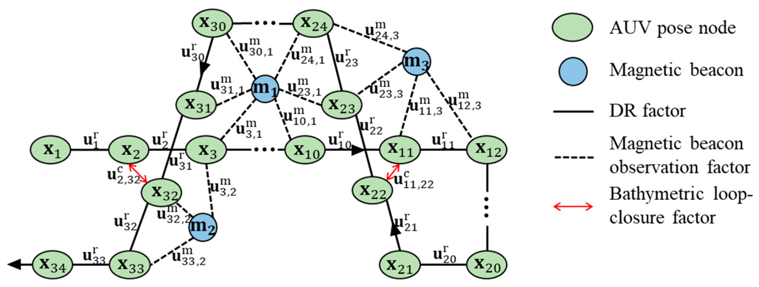
4. Joint-Factor-Graph Construction and Robust Optimization

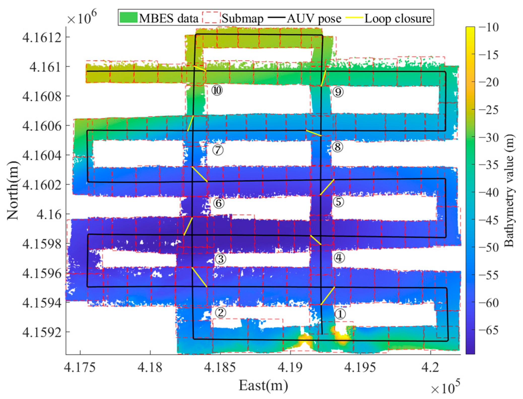
4.1. Joint-Factor-Graph Construction

There are two main kinds of nodes in the joint graph, which are the AUV pose nodes $\mathbf{x}=\{{\mathbf{x}}_i,i=\mathrm{1,2},\dots ,\mathrm{I}\}$ and the magnetic-beacon nodes $\mathbf{m}=\{{\mathbf{m}}_j,j=\mathrm{1,2},\dots ,\mathrm{J}\}$. There are three kinds of factors among the nodes, which are the dead-reckoning (DR) factors ${\mathbf{u}}^{\mathrm{r}}$ between temporally successive AUV pose nodes, the magnetic-beacon-observation factors ${\mathbf{u}}^{\mathrm{m}}$ between AUV pose nodes and magnetic-beacon nodes, and the bathymetric loop-closure factors ${\mathbf{u}}^{\mathrm{c}}$ obtained from multibeam-bathymetric-data association, as illustrated in Figure 4.

The DR factors are obtained from the AUV autonomous navigation systems and the objective function is

$${\mathrm{J}}_{\mathrm{r}}=\sum _i{‖{\mathbf{x}}_i+{\mathbf{u}}_i^{\mathrm{r}}-{\mathbf{x}}_{i+1}‖}_{{\mathsf{\Sigma }}_i^{\mathrm{r}}}^2$$

(35)

where ${\mathrm{J}}_{\mathrm{r}}$ represents the DR factor, ${\mathbf{u}}_i^{\mathrm{r}}={\mathbf{x}}_{i+1}^{\mathrm{D}\mathrm{R}}-{\mathbf{x}}_i^{\mathrm{D}\mathrm{R}}$ is the DR increment between time $i$ and $i+1$, ${‖·‖}^2$ represents the 2-norm of the factor error vector, and ${\mathsf{\Sigma }}_i^{\mathrm{r}}$ is the covariance matrix of the motion-model noise.

The bathymetric loop-closure factors are obtained using the dual-stage bathymetric data-association approach described in Section 2 and the objective function is shown in Equation (36).

$${\mathrm{J}}_{\mathrm{c}}=\sum _{ij}{‖{\mathbf{x}}_i+{\mathbf{u}}_{ij}^{\mathrm{c}}-{\mathbf{x}}_j‖}_{{\mathsf{\Sigma }}_i^{\mathrm{c}}}^2$$

(36)

where ${\mathbf{u}}_{ij}^{\mathrm{c}}$ is the loop-closure measurement, ${\mathsf{\Sigma }}_i^{\mathrm{c}}$ is the covariance matrix of the loop-closure-observation model’s noise. The computation of a bathymetric loop-closure factor is illustrated in Figure 5 and formulated in Equation (37).

$${\mathbf{u}}_{ij}^{\mathrm{c}}={\mathbf{x}}_j^{\mathrm{D}\mathrm{R}}-{\mathbf{x}}_i^{\prime }=\left({\mathbf{x}}_j^{\mathrm{D}\mathrm{R}}-{\mathbf{c}}^{\mathrm{Q}}\right)+\left({\mathbf{c}}^{\mathrm{Q}}-{{\mathbf{R}}^{\ast }\times \mathbf{c}}^{\mathrm{P}}+{\mathbf{t}}^{\ast \ast }\right)+\left({\mathbf{c}}^{\mathrm{P}}-{\mathbf{x}}_i^{\mathrm{D}\mathrm{R}}\right)$$

(37)

The ${\mathbf{x}}_i^{\mathrm{D}\mathrm{R}}$ and ${\mathbf{x}}_j^{\mathrm{D}\mathrm{R}}$ are the AUV positions at moments $i$ and $j$, respectively. The ${\mathbf{c}}^{\mathrm{P}}$ and ${\mathbf{c}}^{\mathrm{Q}}$ are the centers of the source and target submaps. The ${\mathbf{x}}_i\prime$ and ${\mathbf{c}}^{\mathrm{P}}\prime$ are the AUV position and center of the source submap after registration, respectively.

The magnetic beacon observation factors can be obtained by the magnetic-beacon-location approach described in Section 3, and the corresponding objective function is given in Equation (38).

$${\mathrm{J}}_{\mathrm{m}}=\sum _{ik}{‖{\mathbf{x}}_i+{\mathbf{u}}_{ik}^{\mathrm{m}}-{\mathbf{m}}_k‖}_{{\mathsf{\Sigma }}_i^{\mathrm{m}}}^2$$

(38)

where ${\mathbf{u}}_{ik}^{\mathrm{m}}={\mathbf{m}}_k^{\mathrm{o}\mathrm{p}\mathrm{t}}-{\mathbf{x}}_j^{\mathrm{D}\mathrm{R}}$ is the relative position of the magnetic beacons to the vehicle pose nodes. ${\mathsf{\Sigma }}_i^{\mathrm{m}}$ is the covariance matrix of the magnetic beacon observation noise. ${\mathbf{m}}_k$ Indicates the position of the $k$-th magnetic beacon that will be optimized together with the AUV poses in the back-end.

By combining the three kinds of factors together, the general objective function for back-end optimization can be achieved as

$${\mathbf{x}}^{\ast },{\mathbf{m}}^{\ast }={\displaystyle \underset{\mathbf{x},\mathbf{m}}{\mathrm{a}\mathrm{r}\mathrm{g}\mathrm{m}\mathrm{i}\mathrm{n}}}\left({\mathrm{J}}_{\mathrm{r}}+{\mathrm{J}}_{\mathrm{m}}+{\mathrm{J}}_{\mathrm{c}}\right)$$

(39)

4.2. Robust Back-End Optimizer

The bathymetric-loop closures and magnetic-beacon observations generated in the front-end form the observation factor set $\mathcal{F}=\left\{{\mathrm{f}}_1,{\mathrm{f}}_2,\dots ,{\mathrm{f}}_m\right\}$. To identify and exclude potential false factors in $\mathcal{F}$, a diagnosis mechanism is designed and introduced into the back-end optimizer to make it able to detect false factors during optimization. First, some symbols should be defined for clear explanation.

${\mathrm{t}}_n$: the moment that the $n$-th observation factor (bathymetric or magnetic-beacon observation) is obtained.

${\mathrm{L}}_n$: the whole optimized path obtained at ${\mathrm{t}}_n$ using the first $n$ observation factors.

${\mathrm{L}}_n^{-}$: the whole optimized path obtained at ${\mathrm{t}}_n$ using only the first $n-1$ observation factors.

${\mathrm{L}}_{n-1,n}^{-}$: the dead-reckoning path obtained between ${\mathrm{t}}_{n-1}$ and ${\mathrm{t}}_n$.

${\mathrm{L}}_{n-1,n}$: the optimized path section between ${\mathrm{t}}_{n-1}$ and ${\mathrm{t}}_n$.

${\mathrm{P}}_n$: the vehicle position at ${\mathrm{t}}_n$ on ${\mathrm{L}}_n$.

${\mathrm{P}}_n^{-}$: the vehicle position at ${\mathrm{t}}_n$ on ${\mathrm{L}}_n^{-}$.

${\mathrm{P}}_{n-1,n}^{j,-}$: the $j$-th position of the vehicle on ${\mathrm{L}}_{n-1,n}^{-}$.

${\mathrm{P}}_{n-1,n}^j$: the $j$-th position of the vehicle on $L_{n-1,n}$.

$\mathrm{E}\left(\mathrm{P}\right)$: the error ellipse of $\mathrm{P}$.

${\mathrm{b}}_{i,\mathrm{z}}^1,{\mathrm{b}}_{i,\mathrm{z}}^2$: the bathymetric values of the $i$-th closest point pair in the overlapped area of a bathymetric loop-closure.

On the basis of this, a robust back-end optimizer for the joint SLAM is introduced. Once a new observation factor is added into the factor graph and the optimization is updated, a diagnosis mechanism with three conditions will be performed to determine whether the new factor is true and should be reserved. The conditions are given below and illustrated in Figure 6.

Condition 1: $\mathrm{E}\left(\mathrm{P}\right)\cap \mathrm{E}\left({\mathrm{P}}_n^{-}\right)\ne \mathrm{\varnothing }$

Condition 2: $\left|\theta \left({\mathrm{P}}_{n-1,n}^{j,-}\right)-\theta \left({\mathrm{P}}_{n-1,n}^j\right)\right|<{\theta }_{\mathrm{T}}$ for all point pairs on ${\mathrm{L}}_{n-1,n}^{-}$ and ${\mathrm{L}}_{n-1,n}$. The $\theta \left(\ast \right)$ indicates the heading angle at a vehicle position on the path. ${\theta }_{\mathrm{T}}$ is the threshold to judge the heading consistency at points.

Condition 3: $\left(1/n\right)·{\sum }_{i=1}^n\left|{\mathbf{b}}_{i,\mathrm{z}}^1-{\mathbf{b}}_{i,\mathrm{z}}^2\right|<\beta$ for all bathymetric loop-closure areas. $n$ is the number of closest point pairs in a bathymetric loop-closure area and $\beta$ is the threshold used to judge the bathymetric consistency in an overlapped area after optimization

The first condition is to guarantee that the new factor optimizes the DR path in the uncertainty range. If the optimization result is completely outside the error ellipse of the DR estimate, then it is probably a false factor that results in extra errors. The second condition is based on the fact that the underwater navigation systems of AUVs usually have good accuracy. The heading angles of the optimized path should be consistent with the DR path. Otherwise, the path must have been seriously distorted by the newly added factor. The third condition follows the truth that the bathymetric data observed on different paths in a specific area should have strong consistency. False factors lead to wrong positioning estimates and make bad bathymetric consistency at path-cross areas. In summary, only when all of the three conditions are satisfied can the new observation factor be determined as true, and the optimization will be saved for later SLAM solution.

5. Experiment and Analysis

Simulation experiments based on field-multibeam-bathymetric data are conducted to test the joint SLAM approach above. The bathymetric data were surveyed by the authors’ group using a ship equipped with a SONIC 2024 multibeam echo sounder (R2 SONIC, Austin, TX, USA) and a differential GPS receiver (Hi-Target, Guangzhou, China). The GPS path is about 20 km long and include 2868 poses, as shown in Figure 7. In this experiment, the AUV bathymetric survey process and dead-reckoning estimates are simulated using the bathymetric dataset and GPS path.

An ideal AUV DR path is generated first to follow the GPS path, as shown in Equation (40). Then, velocity noise $N\left(0,{0.2}^2\right) \mathrm{m}/\mathrm{s}$ and heading angle noise $N\left(0,{0.02}^2\right) \mathrm{r}\mathrm{a}\mathrm{d}/\mathrm{s}$ are added to simulate an DR path with accumulated errors.

$${\mathbf{x}}_k={\mathbf{x}}_{k-1}+{\mathbf{v}}_k\left[\begin{array}{c}\mathrm{c}\mathrm{o}\mathrm{s}{\phi }_k\\ \mathrm{s}\mathrm{i}\mathrm{n}{\phi }_k\end{array}\right]·∆t$$

(40)

where ${\mathbf{x}}_{\mathit{k}},{\mathbf{v}}_{\mathit{k}}$ and ${\phi }_k$ represent the position, velocity, and heading angle of the AUV at the $k$-th moment, respectively. $∆t$ is the sampling interval and is set to 1 s.

The multibeam-bathymetric data used in simulation is surveyed by us using a SONIC 2024 multibeam echo sounder in a 2 km × 2 km area in the Huanghai Sea, China. The water-depth range of the data set is 5.2~69.8 m and the bathymetric point resolution is about 5 m. Multibeam sonar collects a ping every second and the bathymetric survey process is simulated correspondingly. Nine magnetic beacons are placed in the experiment area in simulation, as shown in Figure 7. The magnetic moments of the beacons are $M_x={10}^6 \mathrm{A}·{\mathrm{m}}^2, M_y={2\ast 10}^5 \mathrm{A}·{\mathrm{m}}^2, {\mathrm{a}\mathrm{n}\mathrm{d} M}_z={10}^5 \mathrm{A}·{\mathrm{m}}^2$. The magnetic strength and gradient data generated by the beacons in the area can be computed using Equations (20) and (21). The magnetometer and gradiometer make measurement at 1 Hz and the measurement noise is set to $N\left(0,{0.1}^2\right)\mathrm{n}\mathrm{T}$.

5.1. Joint-Factor-Graph Construction

During AUV navigation, the magnetic beacons are detected in real time. The magnetic-beacon-location results and the magnetic-beacon-observation factors are shown in Figure 8a,b, respectively. The nine sub-frames in Figure 8a are used to show the magnetic-beacon-detection results clearly. The clustering method based on Euler deconvolution makes good estimations and the optimization approach can further improve the location accuracy. In total, 158 magnetic-beacon observations are reserved in the factor graph and will be taken for back-end optimization.

The multibeam bathymetric strips are divided into 125 submaps, as shown in Figure 9. The minimum submap length $L_{\mathrm{m}\mathrm{i}\mathrm{n}}$ and the maximum submap length $L_{\mathrm{m}\mathrm{a}\mathrm{x}}$ are set to 100 m and 300 m, respectively. The variance of curvature at all bathymetric points in a submap is used to measure the matching suitability $\alpha$. During the multibeam survey, once the submap length satisfies $L_{\mathrm{m}\mathrm{i}\mathrm{n}}\le L\le L_{\mathrm{m}\mathrm{a}\mathrm{x}}$ and the matching suitability $\alpha$ is larger than a threshold ${\alpha }_{\mathrm{t}\mathrm{h}\mathrm{d}}$ the submap construction is completed. The ${\alpha }_{\mathrm{t}\mathrm{h}\mathrm{d}}$ is set to 0.01 in this research.

Two bathymetric loop closures are taken as examples to show the effectiveness of the dual-stage data-association method. The pure GICP method is taken for comparison here. The loop closures labeled with ①, ④, ⑦ and ⑨ in Figure 9 are taken to show the data-association results in Figure 10. The green and blue point clouds indicate the true positions of target and source bathymetric submaps, respectively. The red point cloud represents the registration results obtained using corresponding approaches. Obviously, the closer the red point cloud is to the green point cloud, the higher the bathymetric registration accuracy. For the four loop-closure areas, the dual-stage data-association errors are 4.2 m, 4.8 m, 2.6 m, and 1.5 m, respectively, which are much smaller than those for the GICP results. Then, 100 Monte Carlo data-association experiments are made on the ten submap pairs. The average matching errors of GICP, coarse registration, and dual-stage data-association methods are 14.2 m, 9.1 m, and 4.4 m, respectively. Compared with GICP, the proposed dual-stage method improves the data-association accuracy by 51.7%.

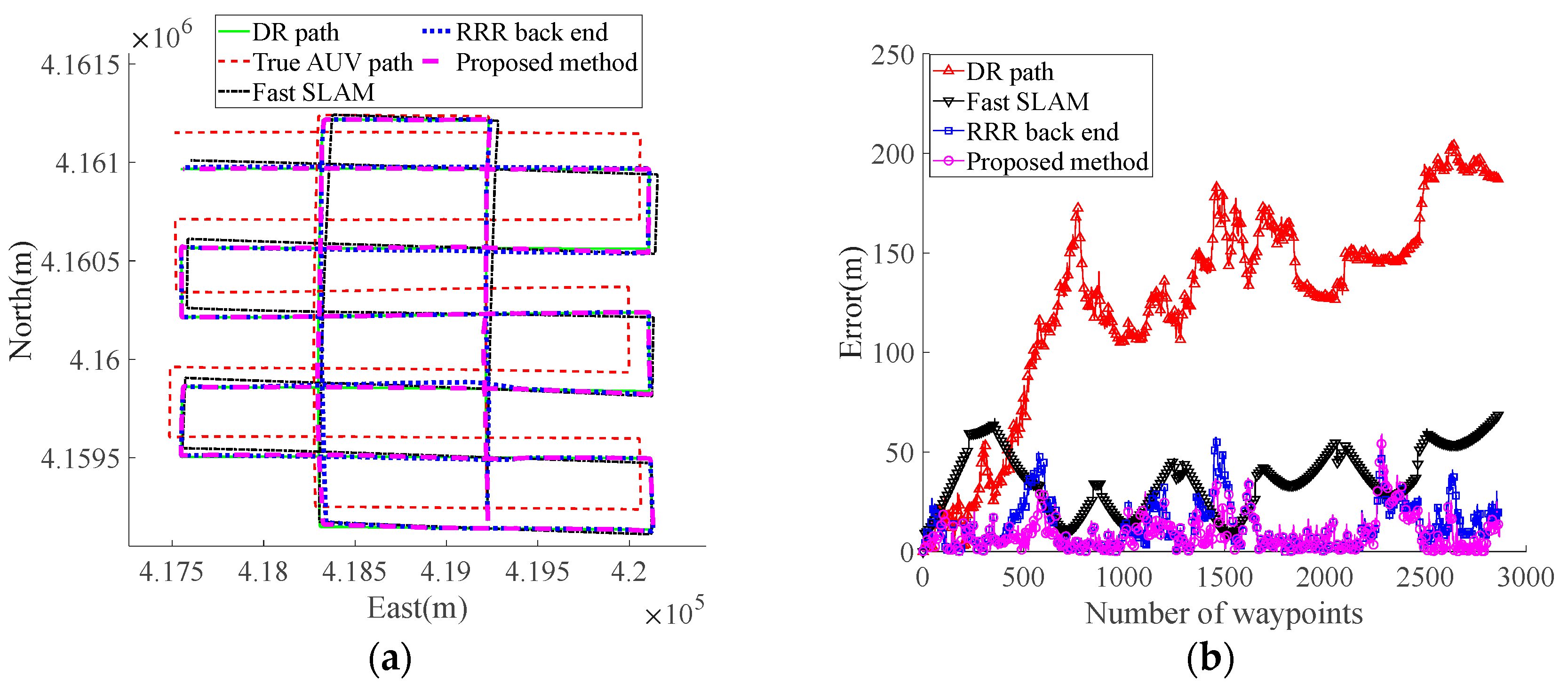
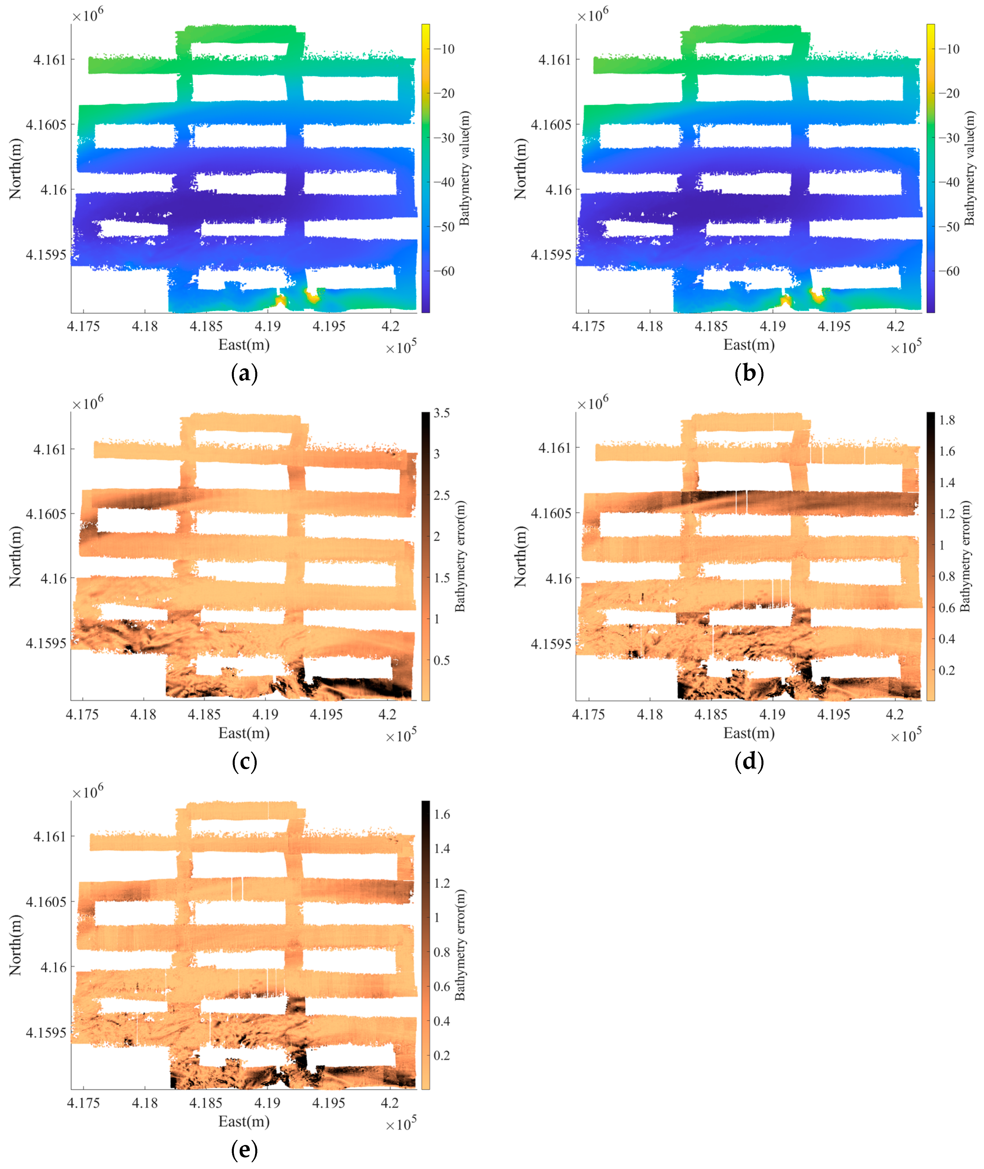
5.2. Back-End Optimization Results

There are 2868 pose nodes, 10 bathymetric loop-closure factors, 2867 DR factors, and 158 magnetic-beacon-observation factors in the factor graph. To verify the significance of magnetic beacons, the factor graph is optimized in two situations. First, all of the factors and nodes in the joint graph are put into the optimizer designed in Section 4.2. Second, only the bathymetric loop-closure and DR factors are used for back-end optimization of pose nodes. The optimization results and errors computed are shown in Figure 11a,b. It can be seen that both situations can give good optimization results that are much closer to the truth than is the DR result. The magnetic beacons can further improve the optimization accuracy compared with the case of using only bathymetric loop closures.

The RRR method [36] and Fast SLAM algorithm [44] are compared at last to evaluate the accuracy and efficiency of the proposed algorithm. Fast SLAM uses 100 particles for filtering estimation. Both the Fast SLAM and RRR methods are performed using the same factor graph with the proposed algorithm. The optimized paths and positioning errors of the three methods are shown in Figure 12. The Fast SLAM method can reduce the DR error to a great extent, but the overall error tends to diverge. The RRR method is able to detect and exclude bad loop closures and has a better performance than Fast SLAM but is inferior to the proposed algorithm. The path estimated by proposed method is the closest to the truth and the average error is less than 10 m. Statistics of the running time of three methods are also made on the computer that has 16G RAM and Intel i7-11700 CPU with 2.5 GHz main frequency. The running time of the proposed SLAM, RRR, and Fast SLAM methods were 521.4 s, 665.6 s, and 752.0 s, respectively.

With the true bathymetric map of the research area shown in Figure 13a as a reference, the mapping errors for pure DR, RRR, Fast SLAM, and the proposed algorithm are computed and shown in Figure 13b–e, respectively. It is obvious that the proposed method has the highest mapping accuracy.

6. Conclusions

To overcome the shortcomings of using pure seabed topographic data in underwater navigation in unknown environments, a joint graph-based underwater SLAM approach that fuses bathymetric and magnetic-beacon observations is proposed in this paper. In the dual-stage bathymetric data association method, the coarse registration method can provide good initialization for the fine registration method using the GICP algorithm. More accurate bathymetric loop closures have been obtained compared with using pure GICP. The combination of Euler-deconvolution method and clustering algorithms make the vehicle able to identify and localize the magnetic beacons deployed on the seafloor accurately. A robust back-end optimizer is also designed to identify the false loop closures in the factor graph. Experiments verified that much better SLAM estimates can be achieved using the proposed joint-factor graph than using classic bathymetric methods. However, there are still some limitations in the paper that need further exploration. The first is that the magnetic-beacon detection is sensitive to environmental noise. Shielding the environmental magnetic-field noise generated by the AUV electronic devices is a challenge. The second is that as the magnetic-field strength decays rapidly with the increase of vehicle-to-beacon distance, it will be difficult to use this method in very large sea areas. We will focus on two works in the near future. The first is combining the geomagnetic anomaly field and magnetic beacons to further enrich the factor graph. The second is improving the robustness of the magnetic-beacon-detection algorithm against environment noises.

References

1. Chutia, S.; Kakoty, N.M.; Deka, D. A Review of Underwater Robotics, Navigation, Sensing Techniques and Applications. In Advances in Robotics; Association for Computing Machinery: New York, NY, USA, 2017; pp. 1–6. [Google Scholar]
2. Sun, K.; Cui, W.; Chen, C. Review of Underwater Sensing Technologies and Applications. Sensors 2021, 21, 7849. [Google Scholar] [CrossRef]
3. Paull, L.; Saeedi, S.; Seto, M.; Li, H. AUV Navigation and Localization: A Review. IEEE J. Ocean. Eng. 2014, 39, 131–149. [Google Scholar] [CrossRef]
4. Zhang, B.; Ji, D.; Liu, S.; Zhu, X.; Xu, W. Autonomous Underwater Vehicle Navigation: A Review. Ocean Eng. 2023, 273, 113861. [Google Scholar] [CrossRef]
5. Deng, Z.; Ge, Y.; Guan, W.; Han, K. Underwater Map-Matching Aided Inertial Navigation System Based on Multi-Geophysical Information. Front. Electr. Electron. Eng. China 2010, 5, 496–500. [Google Scholar] [CrossRef]
6. Chen, P.; Li, Y.; Su, Y.; Chen, X.; Jiang, Y. Review of AUV Underwater Terrain Matching Navigation. J. Navig. 2015, 68, 1155–1172. [Google Scholar] [CrossRef]
7. Zhao, H.; Zhang, N.; Xu, L.; Lin, P.; Liu, Y.; Li, X. Summary of Research on Geomagnetic Navigation Technology. IOP Conf. Ser. Earth Environ. Sci. 2021, 769, 032031. [Google Scholar] [CrossRef]
8. Ånonsen, K.B.; Hagen, O.K. An Analysis of Real-Time Terrain Aided Navigation Results from a HUGIN AUV. In Proceedings of the OCEANS 2010 MTS/IEEE SEATTLE, Seattle, WA, USA, 20–23 September 2010; pp. 1–9. [Google Scholar]
9. Anonsen, K.B.; Hallingstad, O.; Hagen, O.K. Bayesian Terrain-Based Underwater Navigation Using an Improved State-Space Model. In Proceedings of the 2007 Symposium on Underwater Technology and Workshop on Scientific Use of Submarine Cables and Related Technologies, Tokyo, Japan, 17–20 April 2007; pp. 499–505. [Google Scholar]
10. Hagen, O.K.; Ånonsen, K.B. Using Terrain Navigation to Improve Marine Vessel Navigation Systems. Mar. Technol. Soc. J. 2014, 48, 45–58. [Google Scholar] [CrossRef]
11. Meduna, D.K.; Rock, S.M.; McEwen, R. Low-Cost Terrain Relative Navigation for Long-Range AUVs. In Proceedings of the OCEANS 2008, Quebec City, QC, Canada, 15–18 September 2008; pp. 1–7. [Google Scholar]
12. Meduna, D.K.; Rock, S.M.; McEwen, R.S. Closed-Loop Terrain Relative Navigation for AUVs with Non-Inertial Grade Navigation Sensors. In Proceedings of the 2010 IEEE/OES Autonomous Underwater Vehicles, Monterey, CA, USA, 1–3 September 2010; pp. 1–8. [Google Scholar]
13. Roman, C.; Singh, H. Improved Vehicle Based Multibeam Bathymetry Using Sub-Maps and SLAM. In Proceedings of the 2005 IEEE/RSJ International Conference on Intelligent Robots and Systems, Edmonton, AB, Canada, 2–6 August 2005; pp. 3662–3669. [Google Scholar]
14. Roman, C.; Singh, H. A Self-Consistent Bathymetric Mapping Algorithm. J. Field Robot. 2007, 24, 23–50. [Google Scholar] [CrossRef]
15. Huang, Y.; Wu, L.-H.; Sun, F. Underwater Continuous Localization Based on Magnetic Dipole Target Using Magnetic Gradient Tensor and Draft Depth. IEEE Geosci. Remote Sens. Lett. 2014, 11, 178–180. [Google Scholar] [CrossRef]
16. Alimi, R.; Fisher, E.; Nahir, K. In Situ Underwater Localization of Magnetic Sensors Using Natural Computing Algorithms. Sensors 2023, 23, 1797. [Google Scholar] [CrossRef]
17. Chang, S.; Lin, Y.; Fu, X.; Wan, C. A Simultaneous Localization and Mapping Approach Based on Detection of Magnetic Beacons. IEEE Magn. Lett. 2021, 12, 1–5. [Google Scholar] [CrossRef]
18. Chang, S.; Wan, C.; Zhang, D.; Li, H.; Lin, Y. An Underwater SLAM Approach Using Regularly Distributed Magnetic Beacons. In Advances in Guidance, Navigation and Control; Yan, L., Duan, H., Deng, Y., Eds.; Springer Nature: Singapore, 2023; pp. 300–308. [Google Scholar]
19. Du, C.P.; Xia, M.Y.; Huang, S.X.; Xu, Z.H.; Peng, X.; Guo, H. Detection of a Moving Magnetic Dipole Target Using Multiple Scalar Magnetometers. IEEE Geosci. Remote Sens. Lett. 2017, 14, 1166–1170. [Google Scholar] [CrossRef]
20. Wu, M.; Yao, J. Adaptive UKF-SLAM Based on Magnetic Gradient Inversion Method for Underwater Navigation. In Proceedings of the 2015 International Conference on Unmanned Aircraft Systems (ICUAS), Denver, CO, USA, 9–12 June 2015; pp. 839–843. [Google Scholar]
21. Zhao, W.; He, T.; Sani, A.Y.M.; Yao, T. Review of SLAM Techniques for Autonomous Underwater Vehicles. In Proceedings of the 2019 International Conference on Robotics, Intelligent Control and Artificial Intelligence, New York, NY, USA, 20 September 2019; Association for Computing Machinery: New York, NY, USA, 2019; pp. 384–389. [Google Scholar]
22. Hidalgo, F.; Bräunl, T. Review of Underwater SLAM Techniques. In Proceedings of the 2015 6th International Conference on Automation, Robotics and Applications (ICARA), Queenstown, New Zealand, 17–19 February 2015; pp. 306–311. [Google Scholar]
23. Lee, K.-M.; Li, M. Magnetic Tensor Sensor for Gradient-Based Localization of Ferrous Object in Geomagnetic Field. IEEE Trans. Magn. 2016, 52, 4002610. [Google Scholar] [CrossRef]
24. Palomer, A.; Ridao, P.; Ribas, D.; Mallios, A.; Gracias, N.; Vallicrosa, G. Bathymetry-Based SLAM with Difference of Normals Point-Cloud Subsampling and Probabilistic ICP Registration. In Proceedings of the 2013 MTS/IEEE OCEANS—Bergen, Bergen, Norway, 10–13 June 2013; pp. 1–8. [Google Scholar]
25. Palomer, A.; Ridao, P.; Ribas, D. Multibeam 3D Underwater SLAM with Probabilistic Registration. Sensors 2016, 16, 560. [Google Scholar] [CrossRef]
26. Jung, J.; Park, J.; Choi, J.; Choi, H.-T. Bathymetric Pose Graph Optimization With Regularized Submap Matching. IEEE Access 2022, 10, 31155–31164. [Google Scholar] [CrossRef]
27. Bichucher, V.; Walls, J.M.; Ozog, P.; Skinner, K.A.; Eustice, R.M. Bathymetric Factor Graph SLAM with Sparse Point Cloud Alignment. In Proceedings of the OCEANS 2015—MTS/IEEE Washington, Washington, DC, USA, 19–22 October 2015; pp. 1–7. [Google Scholar]
28. Kim, J.; Jung, H.S. An Approach towards Online Bathymetric SLAM. In Proceedings of the OCEANS’11 MTS/IEEE KONA, Waikoloa, HI, USA, 19–22 September 2011; pp. 1–6. [Google Scholar]
29. Barkby, S.; Williams, S.B.; Pizarro, O.; Jakuba, M.V. A Featureless Approach to Efficient Bathymetric SLAM Using Distributed Particle Mapping. J. Field Robot. 2011, 28, 19–39. [Google Scholar] [CrossRef]
30. Callmer, J.; Skoglund, M.; Gustafsson, F. Silent Localization of Underwater Sensors Using Magnetometers. Eurasip J. Adv. Signal Process. 2010, 2010, 1–8. [Google Scholar] [CrossRef]
31. Torroba, I.; Cella, M.; Terán, A.; Rolleberg, N.; Folkesson, J. Online Stochastic Variational Gaussian Process Mapping for Large-Scale Bathymetric SLAM in Real Time. IEEE Robot. Autom. Lett. 2023, 8, 3150–3157. [Google Scholar] [CrossRef]
32. He, B.; Ying, L.; Zhang, S.; Feng, X.; Yan, T.; Nian, R.; Shen, Y. Autonomous Navigation Based on Unscented-FastSLAM Using Particle Swarm Optimization for Autonomous Underwater Vehicles. Measurement 2015, 71, 89–101. [Google Scholar] [CrossRef]
33. Barkby, S.; Williams, S.B.; Pizarro, O.; Jakuba, M.V. Bathymetric Particle Filter SLAM Using Trajectory Maps. Int. J. Robot. Res. 2012, 31, 1409–1430. [Google Scholar] [CrossRef]
34. Ling, Y.; Li, Y.; Ma, T.; Cong, Z.; Xu, S.; Li, Z. Active Bathymetric SLAM for Autonomous Underwater Exploration. Appl. Ocean Res. 2023, 130, 103439. [Google Scholar] [CrossRef]
35. Sünderhauf, N.; Protzel, P. Switchable Constraints for Robust Pose Graph SLAM. In Proceedings of the 2012 IEEE/RSJ International Conference on Intelligent Robots and Systems, Algarve, Portugal, 7–12 October 2012; pp. 1879–1884. [Google Scholar]
36. Latif, Y.; Cadena, C.; Neira, J. Realizing, Reversing, Recovering: Incremental Robust Loop Closing over Time Using the iRRR Algorithm. In Proceedings of the 2012 IEEE/RSJ International Conference on Intelligent Robots and Systems, Algarve, Portugal, 7–12 October 2012; pp. 4211–4217. [Google Scholar]
37. Hitchcox, T.; Forbes, J.R. A Point Cloud Registration Pipeline Using Gaussian Process Regression for Bathymetric SLAM. In Proceedings of the 2020 IEEE/RSJ International Conference on Intelligent Robots and Systems (IROS), Las Vegas, NV, USA, 24 October 2020; pp. 4615–4622. [Google Scholar]
38. Donoso, F.A.; Austin, K.J.; McAree, P.R. How Do ICP Variants Perform When Used for Scan Matching Terrain Point Clouds? Robot. Auton. Syst. 2017, 87, 147–161. [Google Scholar] [CrossRef]
39. Fischler, M.A.; Bolles, R.C. Random Sample Consensus: A Paradigm for Model Fitting with Applications to Image Analysis and Automated Cartography. Commun. ACM 1981, 24, 381–395. [Google Scholar] [CrossRef]
40. Segal, A.; Hhnel, D.; Thrun, S. Generalized-ICP. In Proceedings of the Robotics: Science and Systems V, University of Washington, Seattle, WA, USA, 28 June–1 July 2009. [Google Scholar]
41. Ren, Y.; Hu, C.; Xiang, S.; Feng, Z. Magnetic Dipole Model in the Near-Field. In Proceedings of the 2015 IEEE International Conference on Information and Automation, Lijiang, China, 8–10 August 2015; pp. 1085–1089. [Google Scholar]
42. Teixeira, F.C.; Pascoal, A. Magnetic Navigation and Tracking of Underwater Vehicles. IFAC Proc. Vol. 2013, 46, 239–244. [Google Scholar] [CrossRef]
43. Tran, T.N.; Drab, K.; Daszykowski, M. Revised DBSCAN Algorithm to Cluster Data with Dense Adjacent Clusters. Chemom. Intell. Lab. Syst. 2013, 120, 92–96. [Google Scholar] [CrossRef]
44. Montemerlo, M.; Thrun, S.; Koller, D.; Wegbreit, B. FastSLAM: A Factored Solution to the Simultaneous Localization and Mapping Problem. In Proceedings of the Eighteenth National Conference on Artificial Intelligence, Edmonton, AB, Canada, 28 July–1 August 2002; pp. 593–598. [Google Scholar]
Figure 1. Denoising and down-sampling of bathymetric point cloud. (a) Origin bathymetric point cloud; (b) denoising result; and (c) down-sampling result.
Jmse 12 00954 g001
Figure 2. Schematic diagram of scale selection.  s c a l e _ i   ( i = 1,2 , 3 )  indicates the length of the  i -th square window.
Jmse 12 00954 g002
Figure 3. Procedure of coarse bathymetric point cloud registration.
Jmse 12 00954 g003
Figure 4. Factor graph of the joint SLAM. The arrows indicate the AUV motion direction.
Jmse 12 00954 g004
Figure 5. Calculation of bathymetric loop-closure factor.
Jmse 12 00954 g005
Figure 6. Schematic diagram of false factor detection in back-end.
Jmse 12 00954 g006
Figure 7. Bathymetric map and magnetic-beacon distribution.
Jmse 12 00954 g007
Figure 8. Data association by magnetic-beacon observations. The nine sub-frames in (a) are used to show the relative positions of magnetic-beacon-detection results in enlarged views. (a) Magnetic-beacon-location result; and (b) the magnetic-beacon-observation factors.
Jmse 12 00954 g008
Figure 9. Multibeam submaps and data association. The symbols ① to ⑩ indicate the numbers of loop closures.
Jmse 12 00954 g009
Figure 10. Bathymetric data-association example. The subfigures (a,d,g,j) are the coarse registration results of the loop closures ①, ④, ⑦ and ⑨ in Figure 9. Correspondingly, the subfigures (b,e,h,k) are the fine registration results, and (c,f,I,l) are the registration results using the GICP method.
Jmse 12 00954 g010
Figure 11. Comparison of back-end results with and without magnetic beacons. (a) Comparison of optimized path; and (b) comparison of path errors.
Jmse 12 00954 g011
Figure 12. Comparison of AUV paths using different SLAM methods. (a) Comparison of optimized paths; (b) Comparison of path errors.
Jmse 12 00954 g012
Figure 13. Bathymetric map errors from different methods. (a) True bathymetric map; (b) mapping error of DR; (c) mapping error of Fast SLAM; (d) mapping error of RRR; and (e) mapping error of proposed SLAM.
Jmse 12 00954 g013
Disclaimer/Publisher’s Note: The statements, opinions and data contained in all publications are solely those of the individual author(s) and contributor(s) and not of MDPI and/or the editor(s). MDPI and/or the editor(s) disclaim responsibility for any injury to people or property resulting from any ideas, methods, instructions or products referred to in the content.