Article

Identification of Wind Load Exerted on the Jacket Wind Turbines from Optimally Placed Strain Gauges Using C-Optimal Design and Mathematical Model Reduction

1
Yantai Research Institute, Harbin Engineering University, Yantai 264000, China
2
College of Shipbuilding Engineering, Harbin Engineering University, Harbin 150001, China
*
Author to whom correspondence should be addressed.
J. Mar. Sci. Eng. 2024, 12(4), 563; https://doi.org/10.3390/jmse12040563
Submission received: 4 March 2024 / Revised: 24 March 2024 / Accepted: 24 March 2024 / Published: 27 March 2024
(This article belongs to the Special Issue Ship Motions and Wave Loads—2nd Edition)

Abstract

:
Wind turbine towers experience complex dynamic loads during actual operation, and these loads are difficult to accurately predict in advance, which may lead to inaccurate structural fatigue and strength assessment during the structural design phase, thereby posing safety risks to the wind turbine tower. However, online monitoring of wind loads has become possible with the development of load identification technology. Therefore, an identification method for wind load exerted on wind turbine towers was developed in this study to estimate the wind loads using structural strain, which can be used for online monitoring of wind loads. The wind loads exerted on the wind turbine tower were simplified into six equivalent concentrated forces on the topside of the tower, and the initial mathematical model for wind load identification was established based on dynamic load identification theory in the frequency domain, in which many candidate sensor locations and directions were considered. Then, the initial mathematical model was expressed as a linear system of equations. A numerical example was used to verify the accuracy and stability of the initial mathematical model for the wind load identification, and the identification results indicate that the initial mathematical model combined with the Moore–Penrose inverse algorithm can provide stable and accurate reconstruction results. However, the initial mathematical model uses too many sensors, which is not conducive to engineering applications. Therefore, D-optimal and C-optimal design methods were used to reduce the dimension of the initial mathematical model and determine the location and direction of strain gauges. The C-optimal design method adopts a direct optimisation search strategy, while the D-optimal design method adopts an indirect optimisation search strategy. Then, four numerical examples of wind load identification show that dimensionality reduction of the mathematical model leads to high accuracy, in which the C-optimal design algorithm provides more robust identification results. Moreover, the fatigue damage calculated based on the load identification wind loads closely approximates that derived from finite element simulation wind load, with a relative error within 6%. Therefore, the load identification method developed in this study offers a pragmatic solution for the accurate acquisition of the actual wind load of a wind turbine tower.

1. Introduction

Offshore wind turbine towers confront significant challenges in measuring wind loads due to their intricate designs and the severe operational environments in which they are situated. The complexity of these structures, coupled with the dynamic nature of marine conditions, necessitate precise wind load data. Such data is crucial for evaluating the structural fatigue life of these towers, thereby underscoring the importance of reliable load identification methods [1,2]. Recent advancements in this field have led to the bifurcation of load identification into two principal approaches: time-domain and frequency-domain identifications, each offering unique perspectives on dynamic load analysis [3,4].
Current research within the domain of frequency-domain load identification has progressed from the initial efforts of early investigators [5], expanding its scope to include a variety of engineering structures, such as bridge monitoring [6] and bearing fault diagnosis [7]. This broadening scope demonstrates the increasing applicability and significance of frequency-domain analysis techniques in structural engineering. Frequency-domain methodologies, which are essential for identifying steady-state or stationary stochastic loads, require a comprehensive set of measurement data [8,9]. Moreover, the frequency response function (FRF) matrix, a key component of frequency-domain analysis, tends to exhibit ill-posed resonance points, presenting substantial challenges for numerical precision and stability. Conversely, the time-domain approach, which builds on the system’s dynamic equations, determines the dynamic time history by analysing the complex convolution relationship between excitation and response, effectively avoiding errors from sample truncation, as well as being suitable for identifying non-stationary loads [10,11]. In recent years, as research into load identification technologies has deepened, a variety of innovative methods have been explored and developed, including wavelet transform techniques [12,13], data-driven approaches [4,14], and statistical energy analysis methods [15]. These advancements have significantly improved the accuracy of load identification.
Load identification is an inverse problem. Inverse problems are often ill posed, and regularisation methods have emerged as pivotal for addressing these challenges. Key regularisation techniques include the Tikhonov regularization method (TRM) [16,17], Truncated Singular Value Decomposition (TSVD) [18], and Damped Singular Value Decomposition (DSVD) [19], along with a variety of iterative regularisation approaches, such as the Landweber iteration [20], the Conjugate Gradient iteration [21], and the Least Squares QR (LSQR) iteration method [10].
An alternative approach to addressing ill-posed problems involves the construction of mathematical models with reduced ill posedness. Determining the transfer matrix is the initial step in the identification of stochastic dynamic loads in the frequency domain and dynamic loads in the time domain based on Green’s function, which lays the groundwork for formulating the system of linear equations for load identification. This matrix, serving as the system’s coefficient matrix, significantly influences the solution’s precision. Optimising the transfer matrix by selecting efficient rows (or columns) for matrix inversion is crucial for developing a mathematically robust model. The condition number of the transfer function matrix, indicative of the matrix’s ill posedness, suggests that a lower condition number corresponds to reduced ill posedness. Gupta et al. developed a D-optimal design (DOD) algorithm, leveraging a Sequential Exchange Algorithm (SEA) for strategic sensor positioning and orientation, proven versatile across different structures via numerical examples [22]. Zhang advanced a C-optimal design (COD) method, utilising a Sequential Reduction Algorithm (SRA) for precise sensor placement, aimed at mitigating ill conditioning in mechanical systems [23,24,25,26,27].
Currently, there are relatively few studies on wind load identification for offshore wind turbines, with existing studies focusing on the damage [28], stresses [29], and structural response of wind turbine support structures under external excitation [30]. In his study, Henderson employed a forward analysis approach to calculate the wind loads on offshore wind turbines [31]. The research introduces a reverse calculation strategy to deduce wind loads at the top of offshore wind turbine towers by analysing tower structure response data, offering an effective alternative to direct measurements, particularly under real operational conditions. This study advances the field of frequency-domain random dynamic load identification by proposing a novel technique that utilises response point optimisation algorithms and the Moore–Penrose pseudo-inverse method, thereby constructing mathematical models with inherently lower degrees of ill posedness without relying on traditional regularisation methods. This approach not only improves load identification accuracy but also significantly reduces the sensor count required, aligning with practical engineering needs.
This paper is structured as follows: Section 2 lays the theoretical foundation for wind load identification at turbine tops. Section 3 details the construction of the mathematical model for wind load identification on turbines. Section 4 introduces the method for creating models with lower ill posedness via response point optimisation algorithms. Section 5 validates the feasibility of these algorithms through fatigue analysis of turbine tower structures, utilising the wind load spectrum data derived in Section 4. Section 6 corroborates the proposed method’s effectiveness and accuracy with additional numerical examples. Finally, Section 7 summarises the study’s innovations, acknowledges its limitations, and outlines avenues for future research.

2. Theory of Wind Load Identification for Offshore Wind Turbines

2.1. Frequency-Domain Dynamic Load Identification Theory

Fan blades are continuously exposed to wind loads in offshore jacket wind turbine structures. We decompose these loads into components in six directions ( F x , F y , F z , M x , M y and M z ) to enhance the precision of identifying wind loads on these structures. The wind turbine tower structure is treated as a linear time-invariant system, characterised by a linear relationship between the input (wind load) and the output (structural response). This input-output relationship is articulated as follows [8].
S y y ( ω ) = H ( ω ) S x x ( ω ) H ( ω ) H
where H ( ω ) C n × m symbolises the FRF matrix that encapsulates the physical interrelation between the points of excitation under-identification and the points where responses are measured. ω represent the frequencies. the superscript H represents the conjugate transpose. S x x ( ω ) C m × m is the excitation power spectral density (PSD) matrix, and S y y ( ω ) C n × n is the response PSD matrix.
The relationship between the elements of the response PSD matrix S y y ( ω ) indicates that this matrix is a Hermitian matrix. Matrix S y y ( ω ) can be expressed as follows, based on the properties of Hermitian matrices [8].
S y y ( ω ) = j = 1 r λ j φ j φ j H
where λ j and φ j represent the j-th eigenvalue and eigenvector of the response PSD matrix S y y ( ω ) , respectively. r denotes the rank of the matrix S y y ( ω ) .
The pseudo-response vector r j is constructed as shown in the following equation, utilising each order of eigenpair [8].
r j = λ j φ j e i ω t
where e i ω t denotes a unit harmonic excitation. The response PSD matrix S y y ( ω ) can be transformed as follows [8]:
S y y = j = 1 r r j r j H
The pseudo-response vector r j constructed in Equation (4) can be regarded as generated by a pseudo-excitation vector l j [8]:
r j = H l j
Multiplying both sides of Equation (5) by H + on the left yields the virtual excitation vector l j :
l j = H + r j
where the superscript + denotes the generalised inversion. The excitation PSD matrix S x x ( ω ) can be derived as follows:
S x x ( ω ) = j = 1 r l j l j H

2.2. Ill Posedness of Systems of Linear Equations

Equation (5) is abstracted into an operator equation, A x = y , to analyse the reasons for the emergence of the ill-posed problem in the system of linear equations. Assuming the coefficient matrix is error-free, the operator equation is reformulated due to the inevitable noise present in data collected by sensors in practical scenarios, as follows [32]:
A x + e r r = y δ
where e r r is the error in the response data.
The singular value decomposition of A is performed as follows [32].
A = U S V T = i = 1 n u i s i v i T
where U = ( u 1 , u 2 , , u n ) and V = ( v 1 , v 2 , , v n ) are, respectively, filled with orthonormal columns and satisfy U H U = V H V = I , I is the identity matrix. S = d i a g ( s 1 , s 2 , , s n ) is a non-negative real diagonal matrix, whose diagonal elements are called singular values and are arranged in descending order.
If an inverse matrix exists for the coefficient matrix A , the external excitation can be estimated by substituting Equation (9) into Equation (8) [32]:
x δ = x + i = 1 n s i 1 ( u i T e r r ) v i
In Equation (10), it is evident that errors in the identified excitation occur in two primary domains: (1) smaller singular values result in larger perturbations; and (2) the presence of noise in the response data contributes to a reduction in the accuracy of the identified excitation.
For an operator equation A x = y , the condition number of the coefficient matrix A can serve as an indicator of the degree of ill-posedness, as follows [8].
c o n d ( A ) = A A 1
where A represents the norm of A . Common norms include A 1 = m a x 1 j n i = 1 n | a i j | , A 2 = λ m a x ( A T A ) , and A = m a x 1 i n j = 1 n | a i j | , where λ m a x ( A T A ) denotes the maximum eigenvalue of A T A . In this study, A 2 is utilised to calculate the condition number of matrix A . The larger the condition number, the greater the ill posedness of the linear system.
Another parameter used to assess the degree of ill posedness in a system of linear equations is the determinant obtained through the computation of the transfer matrix A , denoted as D e t ( A ) , as presented in Equation (12) [22]:
D e t ( A ) = A T × A
where A T is the transpose matrix of the transfer matrix A . The larger D e t ( A ) is, the less ill conditioned the linear system becomes.

2.3. Methods for Linear Systems

For the system of linear equations A x = y , if there exists an invertible matrix for A , then x = A 1 y . If there is no invertible matrix for A , then x = A + y . The superscript ‘+’ denotes the Moore–Penrose inverse of the matrix A [33]. The Moore–Penrose pseudo-inverse method is applicable to systems of linear equations that exhibit low levels of ill posedness, whereas systems with severe ill posedness necessitate the use of regularisation methods. From Equation (10), it is evident that the essence of regularisation methods lies in manipulating the smaller singular values. Common direct regularisation methods include TRM and TSVD. Regularisation involves the introduction of a regular operator to mitigate the impact of small singular values.
The regularisation operator for the TRM [32] is
f ( α , s i ) = s i 2 α 2 + s i 2
The corresponding regularisation is
x α , δ = i = 1 n s i ( u i T y δ ) s i 2 + α 2 v i
The regular operator for the TSVD method [18] is
f ( α , s ) = 1 s 2 α 0 s 2 < α
The corresponding regularisation is
x α , δ = s 2 α s i 1 ( u i T y δ ) v i
Both regularisation operators incorporate the regularisation parameter α . The correct selection of the parameters α is crucial and is typically achieved using the L-curve [10] and generalised cross-validation (GCV) criteria [34].
This section summarises five solution methods as follows, each of which has certain limitations and needs to be selected based on the actual situation.
(1)
Moore–Penrose pseudo-inverse method;
(2)
TRM + L-curve: solving a system of linear equations using the TRM, where the regularisation parameter is derived by the L-curve criterion;
(3)
TRM + GCV: solving a system of linear equations using the TRM, where the regularisation parameter is derived using the GCV criterion;
(4)
TSVD + L-curve: solving a system of linear equations using the TSVD method, where the regularisation parameter is derived using the L-curve criterion;
(5)
TSVD + GCV: solving a system of linear equations using the TSVD method, where the regularisation parameter is derived using the GCV criterion.

3. Mathematical Model for Dynamic Load Identification in the Frequency Domain

3.1. Determination of Sensor Orientation

Torsion at the top of a tower results in the distribution of shear stress along the radial direction on the tower surface, as understood from material mechanics principles. Intercepting a micro-element cross-section within the shaft forms a unit body approximated as a positive hexahedron. The absence of stress on the element’s front and rear faces allows for its projection onto a plane parallel to these faces, simplifying the representation of the quadrilateral ABCD, as illustrated in Figure 1. In this configuration, the following relationships hold [35]:
σ x = σ y = 0 ,         τ x y = τ
In the field of material mechanics, the following relationship is established through the outcomes of a two-way stress state analysis [35]:
σ 1 σ 3 = σ x + σ y 2 + ( σ x σ y 2 ) 2 + τ x y 2
t a n 2 α 0 = 2 τ x y σ x σ y
where α 0 is the angle between the direction of the principal stress and the x-axis, which is determined clockwise from the x-axis. σ x , σ y , and τ x y are the transverse, longitudinal, and shear stress components at a point, respectively.
Equation (19) is calculated: α 0 = 4 5 ° or 13 5 ° .
The analyses show that the structural elements oriented at 45° and −45° to the axis endure the maximal tensile and compressive stresses, respectively. Attaching resistive strain gauges at a 45° angle to the inner surface of the tower enhances the precision of the structure’s response. The orientation of the resistive strain gauge at a response point is set to 0°, 45°, and −45° from the axis to enhance the accuracy of structural responses, as illustrated in Figure 2c.
An offshore jacket wind turbine is composed of a jacket foundation, tower, and turbine unit. Ideally, it is assumed that the structural response generated by wind loads at the top of the tower is collected by strain sensors placed on the inner wall of the tower structure, which does not align with reality. Both wave loads and wind loads acting on the surface of the tower, as well as wind loads at the tower’s top, contribute to responses within the tower segment, meaning the structural response captured by actual sensors results from the combined effects of multiple loads. The influence of wave loads and wind loads acting on the tower’s surface on the sensor-collected data is analysed below.

3.2. Analysis of the Effects of Wave Loading on Wind Turbine Structures

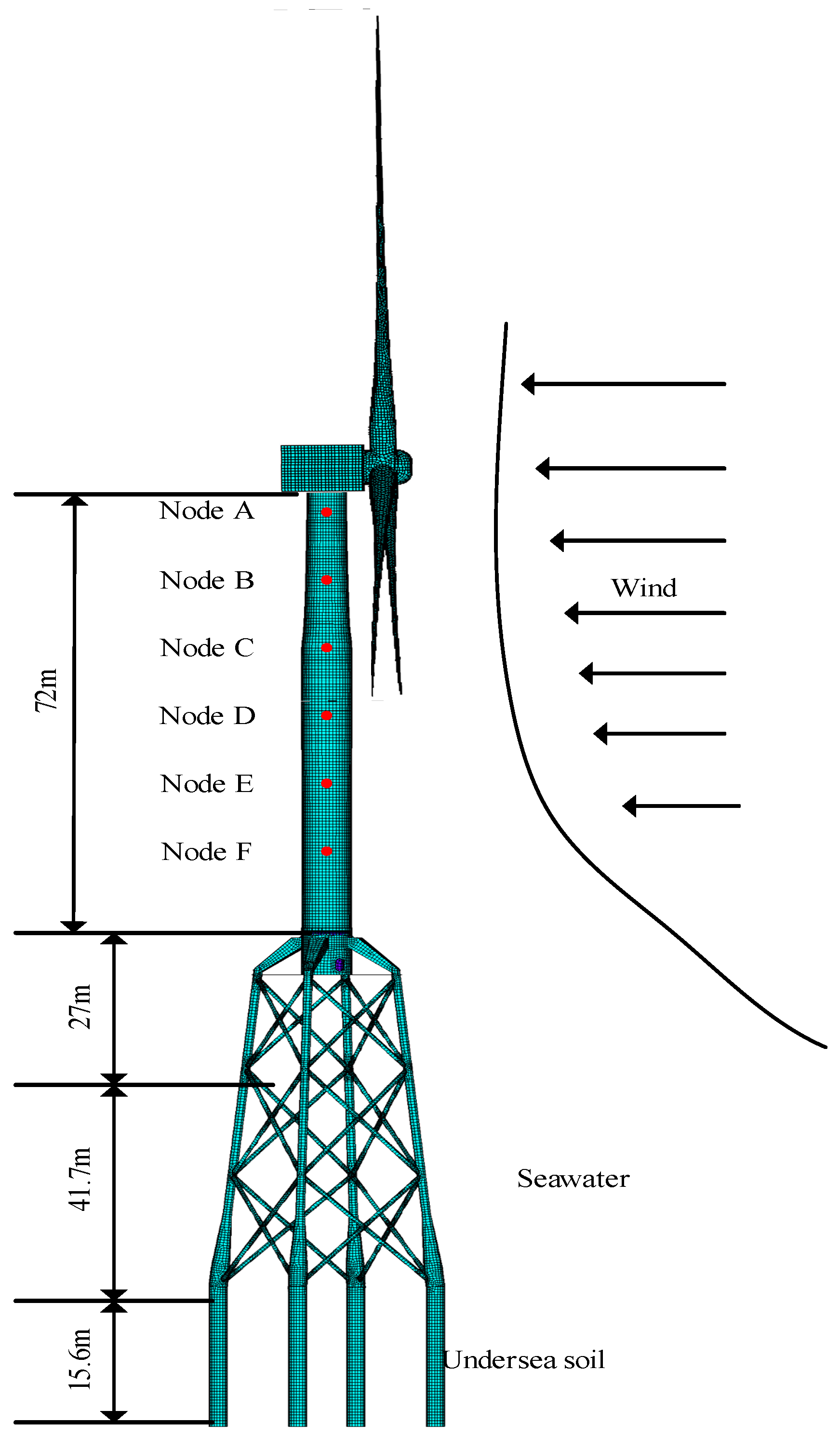
This investigation centred on a wind turbine in the South China Sea, anchored by a jacket-frame foundation. This research aimed at the precise identification of wind loads on this specific turbine, as illustrated in Figure 3. The turbine’s jacket foundation rises to 84.3 m, supported by a 15.6 m pile leg structure embedded in the seabed, while the tower itself soars to a height of 72 m. The following analysis employs Ansys 2022 R1 to examine the effects induced by wave loads.
First, a finite element model (FEM) of the wind turbine structure was created, as depicted in Figure 3. The jacket frame and tower structures were established using shell units, whereas the wind turbine unit was modelled with mass units on the shaft atop the tower.
The joint probability distribution of wind and wave conditions for the specified maritime region is depicted in Figure A1. Analysis of the table reveals the following probabilities: a 29% likelihood for wind speeds under 8 m/s; 18.3% for wind speeds exactly at 8 m/s; 18% for wind speeds of 10 m/s; 12.5% for wind speeds of 12 m/s; and a 22.2% chance for wind speeds exceeding 12 m/s, with a minimal 0.3% probability for extreme wind speeds surpassing 23 m/s. This study selects wind speeds of 8 m/s, 10 m/s, and 12 m/s as the primary scenarios, given their highest probabilities within the joint distribution. With a peak occurrence rate of 5.7% for a 12 m/s wind speed, this study chooses corresponding wave parameters, featuring a wave height of 1.25 m and a period of 4.25 s.
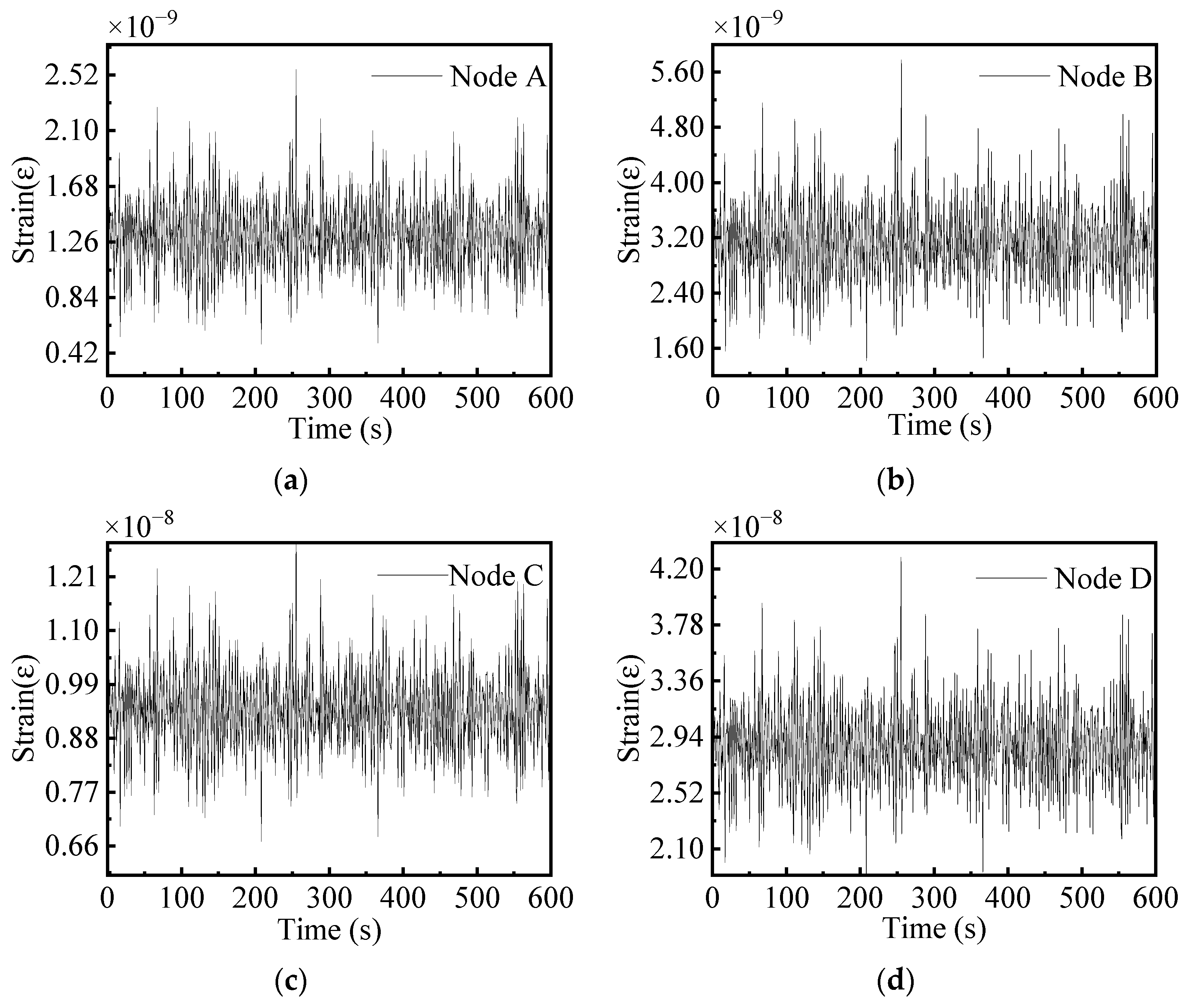
The JONSWAP spectrum [36], a model designed to characterise the energy distribution of sea waves, is employed. Utilising the chosen wave parameters, this study conducts wave condition simulations within the Ansys Aqwa environment based on the JONSWAP spectrum for the defined maritime area. The calculated wave load was then applied to the FEM of the entire wind turbine structure, initiating a transient dynamics analysis to determine the structural response of the entire system under the wave load. The first principal strain data for the six nodes of the tower structure is shown in Figure 4.
The strain range observed in the tower structure was 1 0 9 1 0 7 under wave loading. It is noted that the structural response to wave loads decreases progressively towards the upper sections of the tower. The impact of wave loading on the wind turbine tower’s structural behaviour is considered negligible, due to resistance strain gauges’ limitation in detecting strains smaller than 1 0 6 .

3.3. Effects of Wind Loads on Wind Turbine Tower Structures

The structural response of the tower in practical operation is commonly influenced by the combined effects of wave loads, wind loads at the tower’s top, and wind loads on the tower surface. This study simplifies the analysis by assuming the structural response is primarily due to wind loads at the top. Preliminary analysis indicates that the impact of wave loads on the structural response is relatively minor, and thus, it is neglected in further studies. This section focuses on the impact of wind loads on the tower surface on the structural response, conducting a detailed simulation analysis using Ansys software.
Winds within the atmospheric boundary layer near the Earth’s surface impact structures in two primary forms: mean winds and fluctuating winds. Mean winds, responsible for static loads, can lead to wind-induced vibrations, vortex-induced vibrations, and stability issues under static conditions. Fluctuating winds, on the other hand, are key in driving dynamic responses, notably in bridges. The velocity of wind within this layer varies complexly with elevation due to the frictional effects of surface roughness, showing an increase in mean velocity with altitude. Dynamic factors like surface roughness and thermal factors such as atmospheric stability, which are often represented by logarithmic or exponential profiles, intricately affect this vertical distribution of mean wind velocity [37,38]. In the surface layer, which reaches up to 300 m above ground, variations in shear stress are deemed negligible, simplifying the representation of the wind velocity profile to the following relationship [39]:
U ( z ) = u k l n ( z z 0 ) + 5.75 z z g
where U ( z ) is the mean wind speed at height z above the ground, u is the friction velocity, u = 0.775   m / s , k is the Karman constant, k 0.4 , z 0 is the ground roughness length, and z 0 = 0.01 , z g is the gradient height, it can be considered that the wind velocity assumes a constant value when the altitude exceeds the gradient height. z g = 0.175 u / f c f c is the Coriolis constant, f c = 2 ω s i n Φ , ω is the angular velocity of Earth’s rotation, ω = 7.27 × 1 0 5   r a d / s , and Φ is the latitude.
The nature of wind inflow is intrinsically time-variant, and spectral methods are prevalently utilised to simulate the temporal fluctuations in inflow characteristics. Employing empirical wind field data sourced from coastal regions in China, the subsequent horizontal fluctuating wind speed spectrum is proposed for modelling the temporal variations in wind velocity [40]:
n S u ( n ) σ u 2 = 23.41 f ( 1 + 30.63 f ) 5 / 3
where S u ( n ) is the horizontal wind speed power spectrum, n is the frequency, σ u is the horizontal pulsating wind speed root variance, σ u 2 = 0.05 + 1.26 u 2 , f = n z / U is the dimensionless frequency (also known as the Monin similarity coordinate), and U is the mean wind speed.
The computational domain’s dimensions were meticulously defined for simulations with Ansys Fluent 2022 R1, as illustrated in Figure 5a, to closely mimic realistic environmental conditions. The domain’s extensive span of 3000 m in length, 1600 m in width, and 1500 m in height, with 500 m upstream and 2500 m downstream, was chosen based on preliminary tests to ensure minimal boundary effects on the simulation results. Figure 5b–d showcase the finite volume models, illustrating a comprehensive approach to capturing the complex fluid dynamics around the turbine. The inlet wind speed, crucial for accurate load simulation, was determined using Equations (20) and (21). Simulations conducted at a granular 0.01 s time step over 100 s offered high-resolution insights into the wind load dynamics. Post-processing involved considering the tower’s top generator set and fan blades as a mass point to streamline the analysis without compromising accuracy.
A fundamental assumption of this study is that the tower structure is primarily influenced by wind loads at the top of the tower. Two sets of transient dynamic analyses were conducted to verify this hypothesis in Ansys. In the first set, the wind loads in the six directions extracted in the previous step were applied to the mass point at the top of the tower, along with the pressure from the wind field applied to the surface of the tower. In the second set, the wind loads in the six directions were applied solely to the mass point at the top of the tower.
The tower structure was segmented into four parts: windward, leeward, and two sideward surfaces in this study. Nodes 1 to 6 represent the 6 nodes on the windward face arranged from top to bottom, Nodes 7 to 12 correspond to the sideward face 1 in the same top-down arrangement, Nodes 13 to 18 for the leeward face, and Nodes 19 to 24 for the sideward face 2. This research compared two sets of data to assess the simulation of the tower structure’s response: the first set provides a more comprehensive structural response, whereas the second offers a simplified version. Given the preference for simplified data processing methods in practical engineering applications, this study explored the feasibility of substituting the first set of data with the second. The difference obtained by subtracting the second set of data from the first was considered noise, and this study further analysed its proportion relative to the first set. The noise level was assessed using the signal-to-noise ratio (SNR), which is the ratio of signal power to noise power, measured in decibels (dB). A higher SNR indicates lesser noise within the signal. The calculated SNR values for the 24 nodes are shown in Table 1, where the second column represents the SNR values for the structural response in the direction parallel to the axis, the third column for the response at a 45 angle to the axis, and the fourth column for the response at a −45 angle.
Overall, the SNR values span approximately from 24 dB to 56 dB, with the minimum SNR value being 24.7581 dB, observed in the direction at a 45° angle to the axis at Node 12; the maximum SNR value reaches 56.9636 dB, noted in the direction parallel to the axis at Node 16. There is a general tendency for the SNR to increase with elevation, examining the trend along the height of the tower. This pattern suggests that the structural responses in the lower regions of the tower are more influenced by wind loads on the tower’s surface, indicating a higher contribution of surface wind loads to the structural response in these areas. Conversely, the top regions of the tower are less affected by surface wind loads. Observing from the perspective of sensor orientation, the SNR values in directions parallel to the tower’s axis are higher than those in the other two directions, indicating lower noise levels and a reduced impact of surface wind loads in the axial direction.

3.4. Determination of Initial Sensor Position

The analysis clearly demonstrates a reduction in the noise levels within the measured structural response data as the placement of the sensors ascends towards the tower’s upper, as initially depicted in Figure 2. The tower, standing at a height of 72 m, required a careful strategy to minimise the effects of both wave and wind loads on its structural integrity. Consequently, sensors were methodically arranged at vertical intervals of 3 m, starting from a height of 24 m up to the tower’s full height of 72 m. At each specified level, the sensors were uniformly distributed in a circumferential pattern at intervals of 15 degrees, resulting in a configuration of 24 sensors for each circular layer. This comprehensive setup resulted in a total of 16 sensor layers, culminating in an extensive network of 1152 sensors.

3.5. Mathematical Modelling and Analysis of the Effects of Load Identification

The process of constructing a wind load identification model for wind turbines is illustrated through the following steps, using the structure described above as an example.
Step 1: Analyses in Section 3.3 indicate that offshore wind turbines primarily face aerodynamic blade loads during actual operations. This study adopted GH Bladed 4.3, renowned for its foundation in blade momentum theory, for the aerodynamic load analysis of offshore wind turbines, due to the slow calculation speed of Ansys Fluent software. GH Bladed demands inputs like blade specifications, airfoil details, tower characteristics, generator set properties, and wind conditions for accurate calculations. The model parameters of the blades are listed in Table 2.
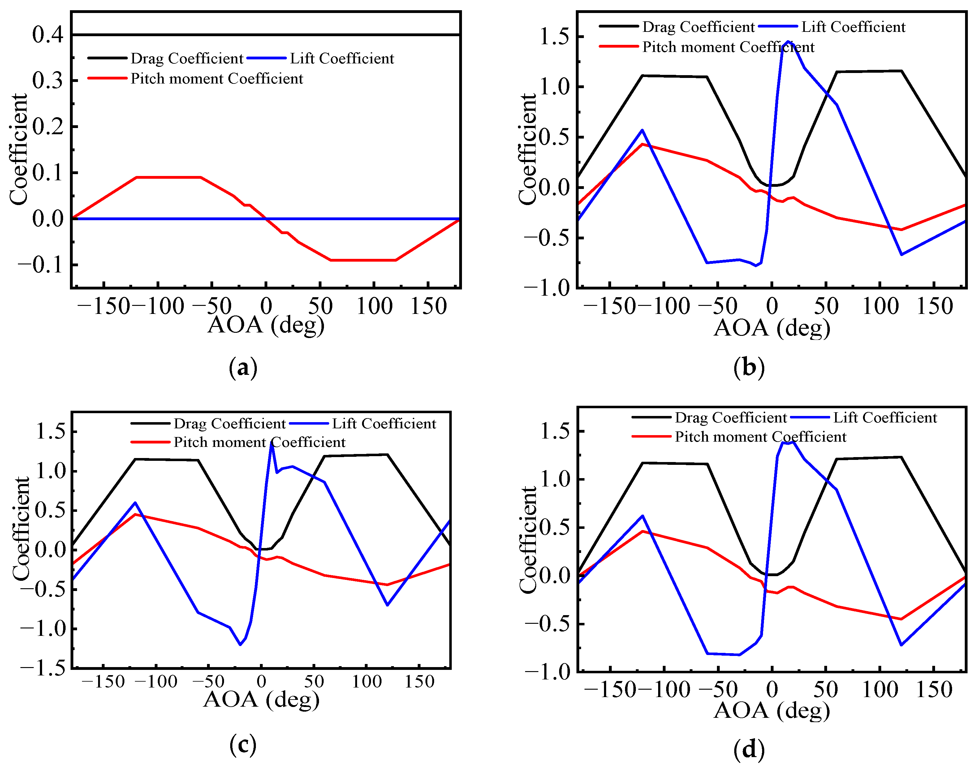
The graphs depicting the variations in the lift and drag coefficients with respect to the angle of attack (AOA) for the four airfoil cross-sections outlined in Table 2 are presented in Figure 6.
The mass and stiffness parameters of the blades are shown in Table 3.
The complexity of the airflow around offshore wind turbines necessitates selecting a suitable turbulence model. This study used the GH Bladed software, opting for the improved von Karman model’s longitudinal component. Table 4 lists the model’s parameters, specific to the project’s location.
The time-course curve for the wind loads was computed following the outlined procedures. This calculation was conducted with an average wind speed of 8 m/s, a duration of 600 s, and a time step of 0.02 s, as illustrated in Figure 7.
Step 2: The wind load components ( F x , F y , F z , M x , M y , and M z ) were imposed on the mass cell utilising Ansys software, initiating transient dynamics calculations on the structure to extract stress-time data at specific nodes. The stress data parallel to the axial direction of the tower are denoted as y 1 ( t ) , y 2 ( t ) , , y 384 ( t ) , the data at a −45° angle to the axial direction are represented as y 385 ( t ) , y 386 ( t ) , , y 768 ( t ) , and the data at a 45° angle to the axial direction are denoted as y 769 ( t ) , y 770 ( t ) , , y 1152 ( t ) . Autocorrelation and cross-correlation functions were computed for these datasets, followed by a Fourier transformation based on the Wiener–Sinchin theorem [41] on the resultant outcomes to derive the spectral matrix of the response of the structure. For example, the autocorrelation and cross-correlation functions were calculated for y 1 ( t ) and y 2 ( t ) , and a Fourier transform was applied to obtain S y 1 , S y 2 , S y 1 y 2 , and S y 2 y 1 . Their positions in the response spectrum matrix S y y were designated as (1,1), (2,2), (1,2), and (2,1), respectively.
Step 3: Harmonic response analyses were conducted using ANSYS software, where six distinct unit load components were applied individually to the mass unit. The real and imaginary parts of the micro-strain response generated by the structure at the monitoring point locations for each frequency were extracted and amalgamated into complex numbers. The responses at the monitoring site were denoted as H y 1 x 1 , H y 2 x 1 , H y 1152 x 1 ( F x direction), H y 1 x 2 , H y 2 x 2 , H y 1152 x 2 ( F y direction), H y 1 x 3 , H y 2 x 3 , H y 1152 x 3 ( F z direction), H y 1 x 4 , H y 2 x 4 , H y 1152 x 4 ( M x direction), H y 1 x 5 , H y 2 x 5 , H y 1152 x 5 ( M y direction), and H y 1 x 6 , H y 2 x 6 , H y 1152 x 6 ( M z direction). A frequency response function matrix H , with dimensions of 1152×6, was constructed by employing the combination rule outlined in Step 2.
Step 4: Five distinct inverse methods were applied to calculate the wind loads in Equation (22). Each method offers unique advantages in addressing ill-posed problems and improving solution stability. A comparative analysis was conducted to identify the most effective approach for the specific application. The optimal method was selected based on its overall performance across these criteria, ensuring the most reliable wind load computation.
S y 1152 y 1152 = H y 1152 x 6 × S x x × H y 1152 x 6 H
TRM + L-curve was used to solve Equation (22), and the load identification results are presented in Figure 8.
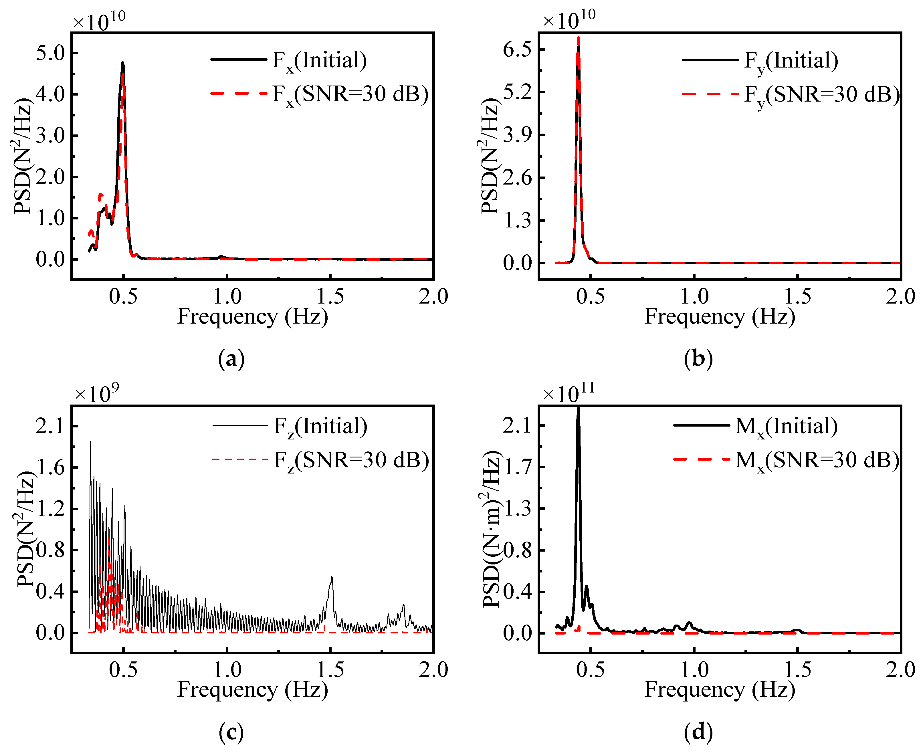
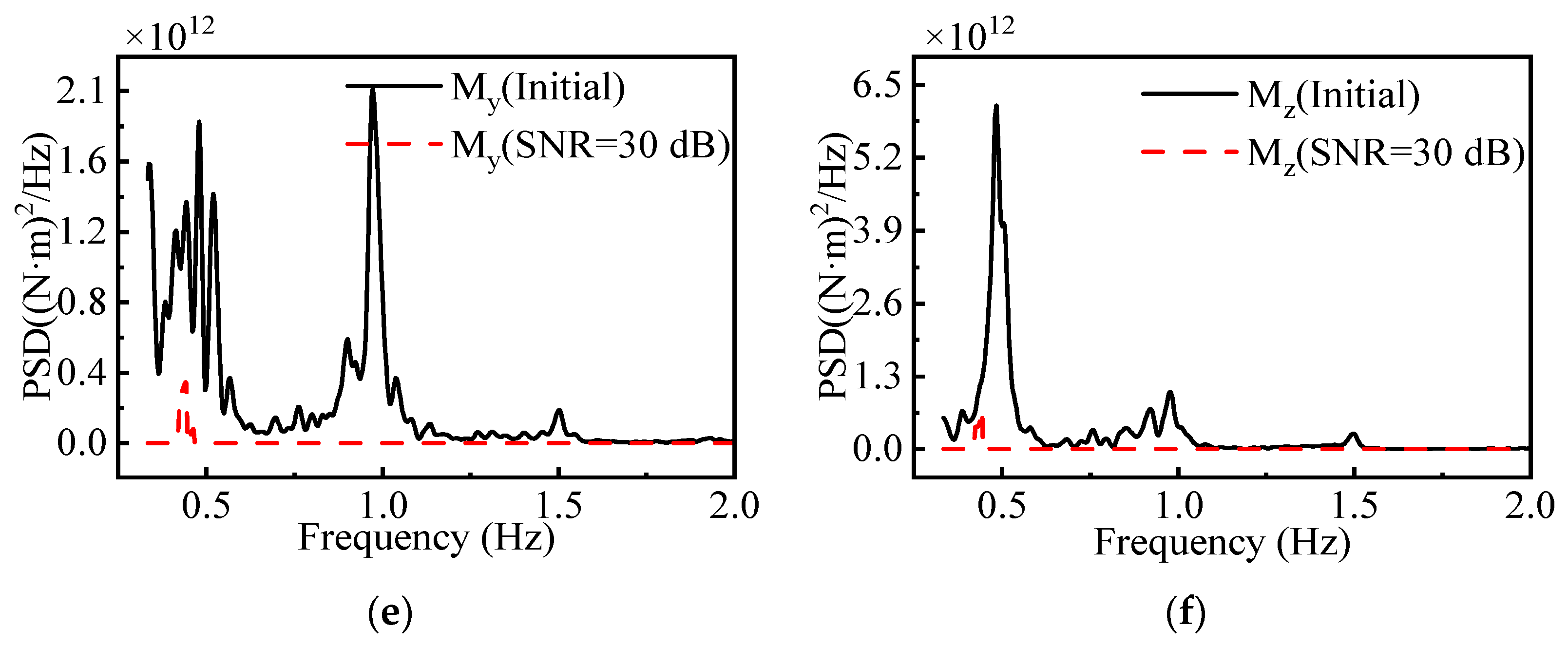
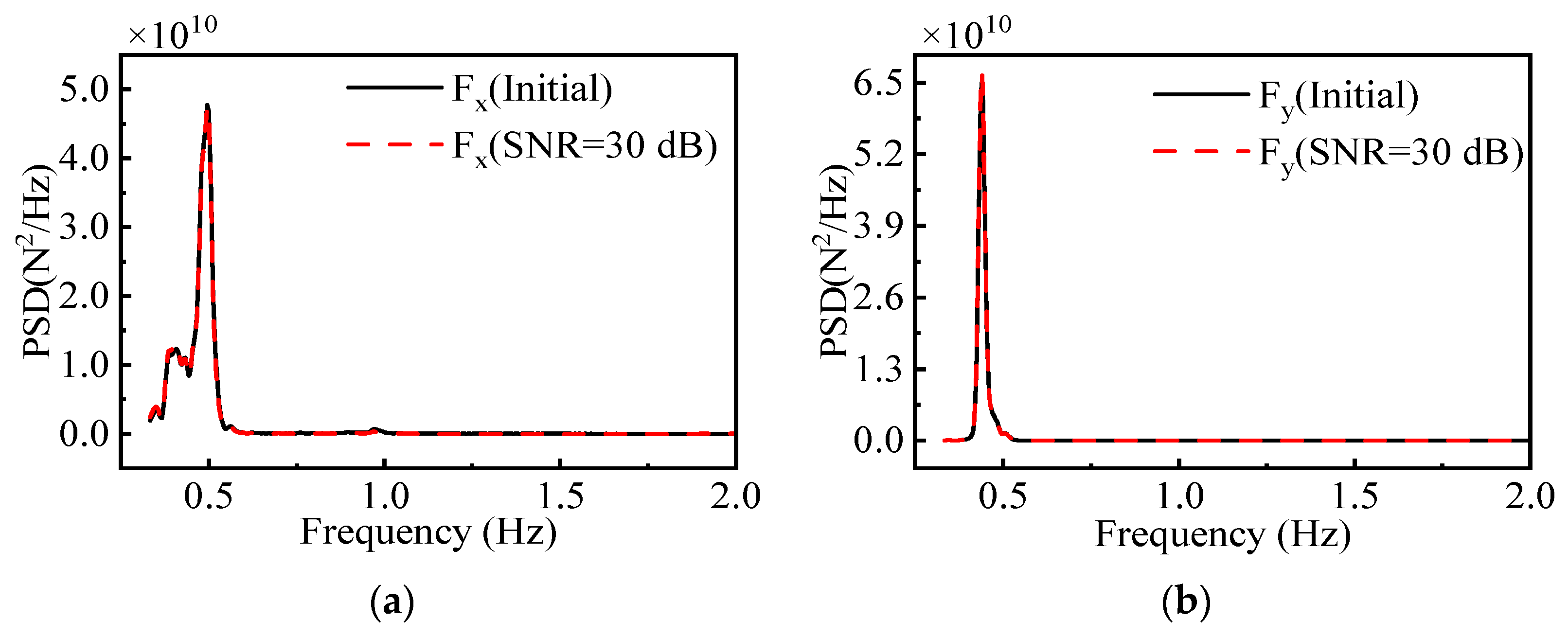
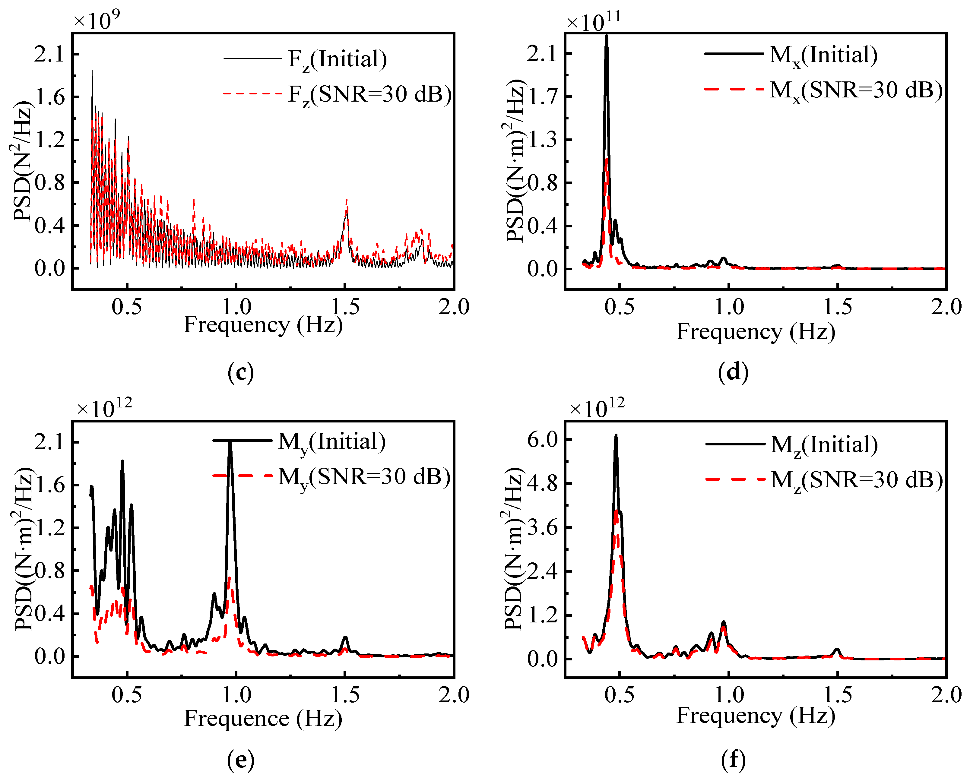
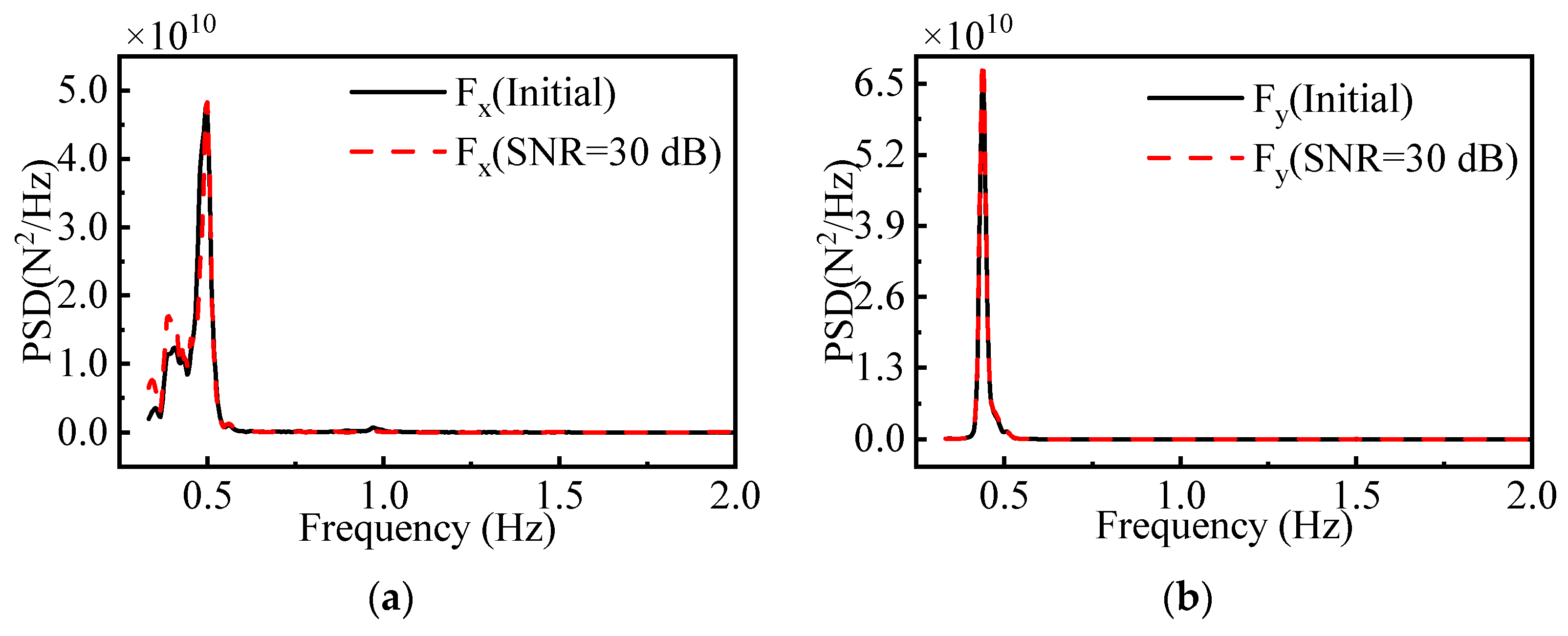
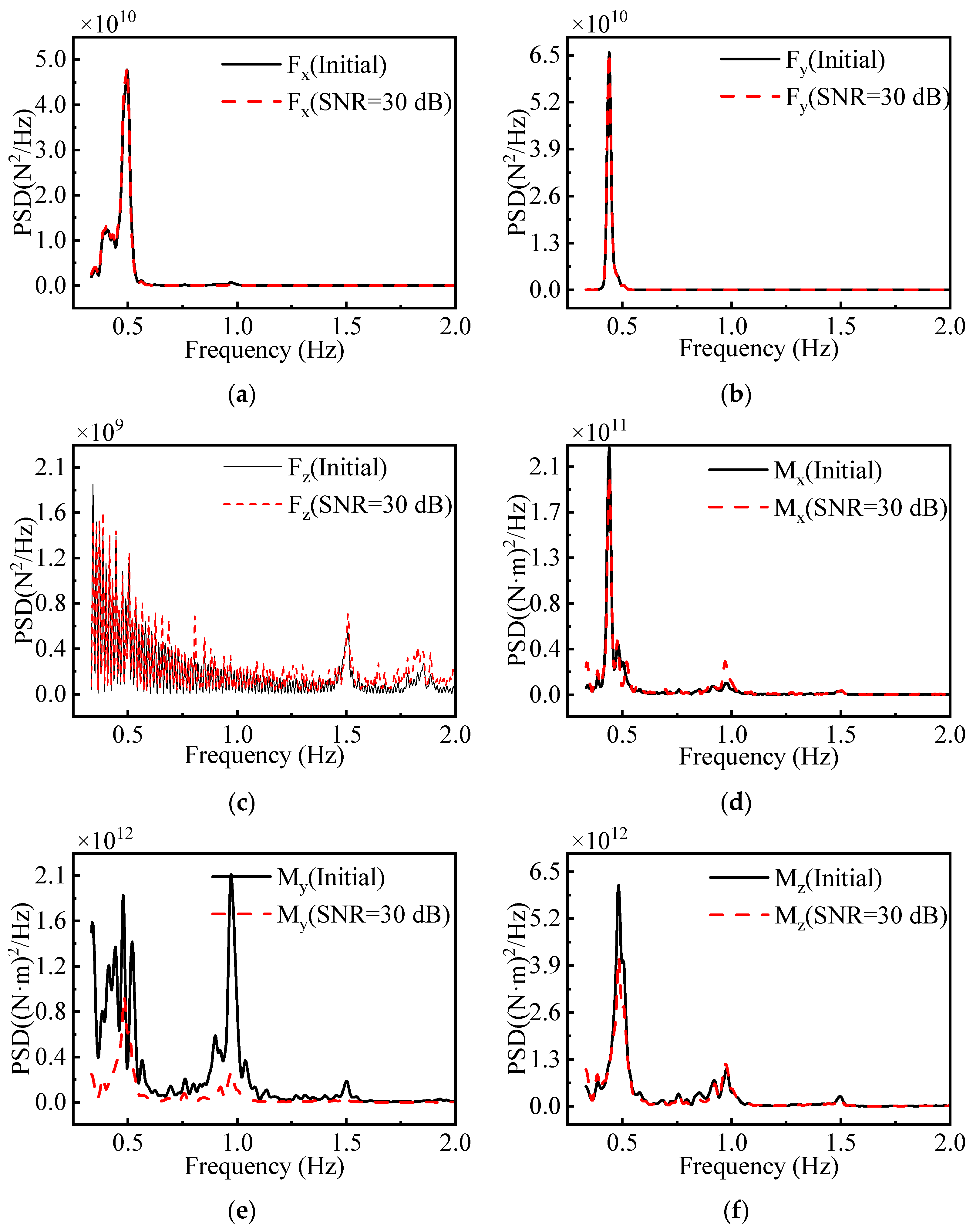
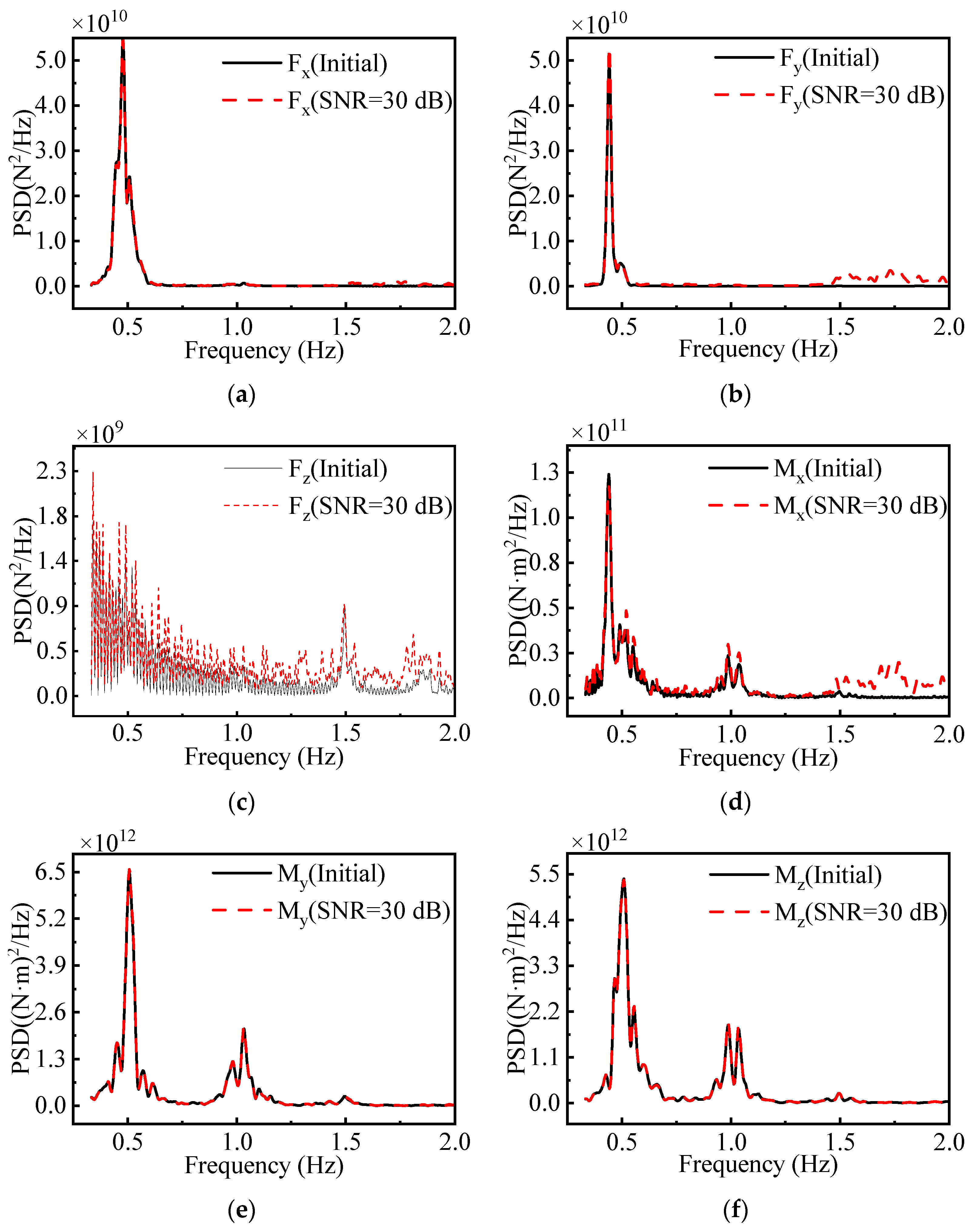
The preceding analysis led to the assumption that the wave load had a negligible effect on the sensor-monitored data from the tower structure. However, the wind load directly impacting the tower surface influenced the sensor-monitored data, with SNR values ranging approximately between 30 and 50 dB, approaching 40 dB. Additionally, the sensors themselves contributed to the overall noise. Gaussian white noise [42] was introduced to the structural response data from the finite element calculations, with the SNR set at 30 dB, to enhance the realism of the simulation experiments. Figure 9 illustrates that the load spectra were accurately identified in the F x and F y directions, yet identification was less effective in the F z , M x , M y , and M z directions. This observation indicates the inefficacy of the TRM + L-curve method for the given load identification mathematical model.
TRM + GCV was used to solve Equation (22), and the load identification results are shown in Figure 9.
TSVD + L-curve was used to solve Equation (22), and the load identification results are presented in Figure 10.
The identified load spectra in the F x and F y directions were closely aligned with the initial wind load spectra, revealing a higher accuracy in load identification. However, in the F z direction, there was a noticeable deviation between the identified and initial load spectra. In the M x , M y , and M z directions, the identified load spectra exhibited significant disparities from the initial wind load spectra. This disparity was particularly pronounced around 0.5 Hz and 1.0 Hz, corresponding to peaks in the actual wind load spectrum. Notably, there was a substantial gap between the identified load and initial wind load spectra during these peak frequencies. Overall, the load spectrum identified using the TSVD + L-curve solution method lacked accuracy.
TSVD + GCV was used to solve Equation (22), and the load identification results are presented in Figure 11.
In the F x and F y directions, the identified load spectra exhibited a strong correspondence, particularly in the 0.5 Hz region, where the initial wind load spectrum peaked. This resulted in effective overall identification. Conversely, in the F z direction, there was a noticeable deviation between the identified load and initial wind load profiles, primarily observed in the frequency range from 0.5 to 2 Hz, where the power of the load profiles was comparatively lower. For the M x and M z directions, the identified load profiles demonstrated high overall accuracy, although a slight decrease in accuracy occurred around 0.5 Hz and 1.0 Hz. However, the M y direction generally exhibited poor performance with low accuracy in the identified load spectrum. In conclusion, the TSVD + GCV solution method proved unsuitable.
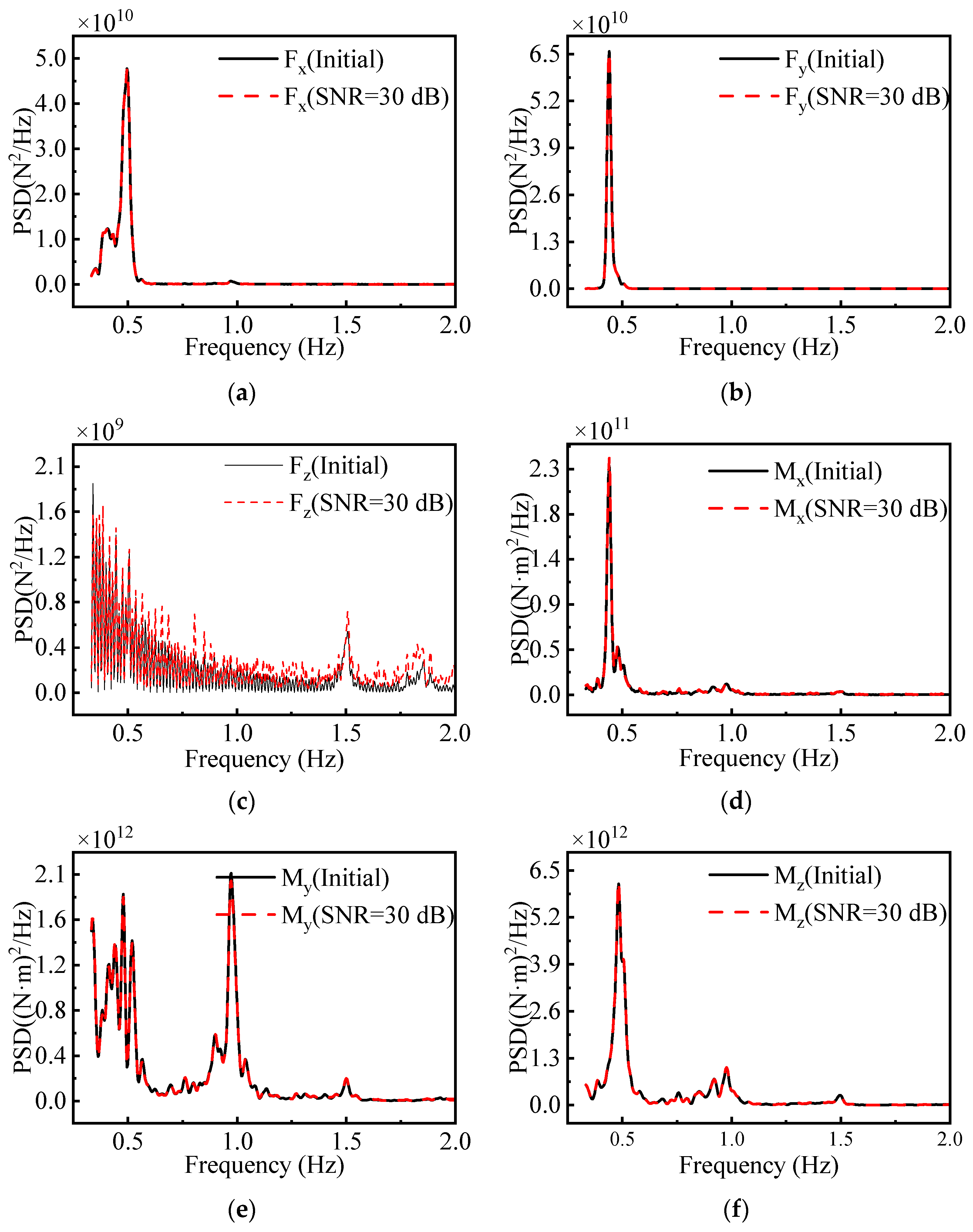
The Moore–Penrose pseudo-inverse method was used to solve Equation (22), and the load identification results are presented in Figure 12.
In the F x , F y , M x , M y , and M z directions, the identified load spectra closely resembled the actual load spectra, revealing a high level of accuracy in load identification. However, in the F z direction, load identification was less effective, as is evident in the power spectrum in Figure 12. The power spectrum in the F z direction had an order of magnitude represented by 1 0 9 , significantly differing from the magnitudes observed in the other five directions. Although the load identification in this direction was suboptimal, its impact on the overall accuracy was minimal. The Moore–Penrose inverse method exhibited excellent solution accuracy and noise immunity within the context of this mathematical model.
M A E ( X , h ) = 1 m i = 1 m | h ( x i ) y i |
Mean absolute error (MAE) denotes the average of the absolute errors between the predicted and initial values [43], as shown in Equation (23). A comparative analysis, utilising Mean absolute error (MAE) as the evaluation criterion and detailed in Table 5, was conducted to discern the optimal solution method among the five options.
The analysis of data from Table 5 and Figure 12 reveals that in the F x and F y directions, where the original load spectrum peaks were of magnitude 1 0 10 , the Moore–Penrose pseudo-inverse method exhibited identification errors of magnitude 1 0 7 , which were lower than the errors from the other four methods. In the F z direction, with original load spectrum peaks of magnitude 1 0 9 , the identification errors of the Moore–Penrose pseudo-inverse method, of magnitude 1 0 7 , were comparable to those of the other four methods. For the M x direction, where the original load spectrum peaks were of magnitude 1 0 11 , the Moore–Penrose pseudo-inverse method’s identification errors, of magnitude 1 0 7 , were lower than those of the other methods. Furthermore, in the M y and M z directions, with original load spectrum peaks of magnitude 1 0 12 , the identification errors of the Moore–Penrose pseudo-inverse method, of magnitude 1 0 9 , were significantly lower than those of the other four methods. Overall, the magnitude of identification errors from the Moore–Penrose pseudo-inverse method was 2 to 3 orders lower than the magnitude of the original load spectrum peaks. This finding indicates that the Moore–Penrose pseudo-inverse method offers enhanced accuracy and stability within the mathematical model developed for this study.

4. Sensor Arrangement Optimisation Methods

The Moore–Penrose pseudo-inverse method enhances load identification accuracy, yet optimising sensor arrangements is crucial due to the extensive sensor data in engineering. This study identified inefficient data points within the linear equation system for removal. Both COD and DOD methods were used for sensor optimisation. This led to a reduction in sensors from 1152 to 6. The COD method simplifies matrix conditions measurement, using a SRA to efficiently filter matrices, as detailed below [44]:
(1)
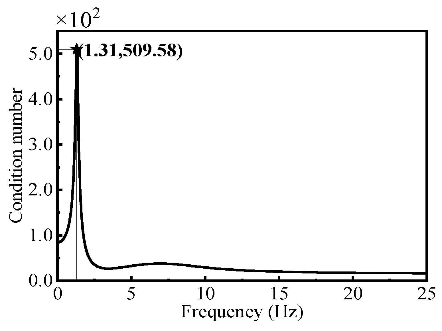
For the variation in the condition number of H n × m in the initial mathematical model, as shown in Figure 13, the frequency response function matrix corresponding to the maximum condition number is selected. For this frequency response function matrix H n × m , compute all its remaining matrices to obtain H 1 ( n 1 ) × m , H 2 ( n 1 ) × m ,..., and H n ( n 1 ) × m .
(2)
Calculate all remaining condition numbers of the matrix H n × m , that is, the condition numbers of H 1 ( n 1 ) × m , H 2 ( n 1 ) × m ,..., and H n ( n 1 ) × m .
(3)
Select the residual matrix corresponding to the smallest number of residual conditions; that is, the matrix H n × m becomes H ( n 2 ) × m , completing the first reduction.
(4)
Calculate all remaining condition numbers of the matrix H ( n 1 ) × m , that is, the condition numbers of H 1 ( n 2 ) × m , H 2 ( n 2 ) × m , …, and H n ( n 2 ) × m .
(5)
Select the residual matrix corresponding to the smallest residual condition number; that is, the matrix H ( n 1 ) × m becomes H ( n 2 ) × m , completing the second reduction.
(6)
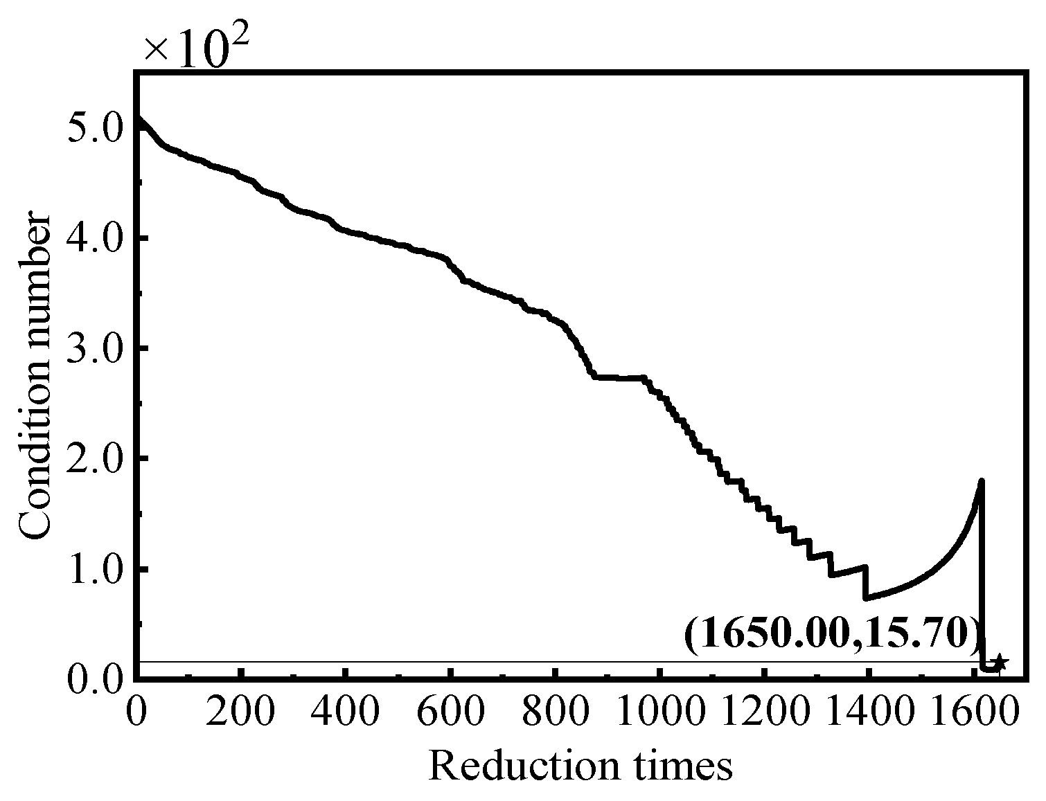
This continues until the matrix H n × m is reduced to H p × m . The change in the frequency response function matrix condition number as the number of reductions increases is shown in Figure 14. As shown in this figure, the condition number decreased from more than 500 to approximately 15, showing an obvious change.
(7)
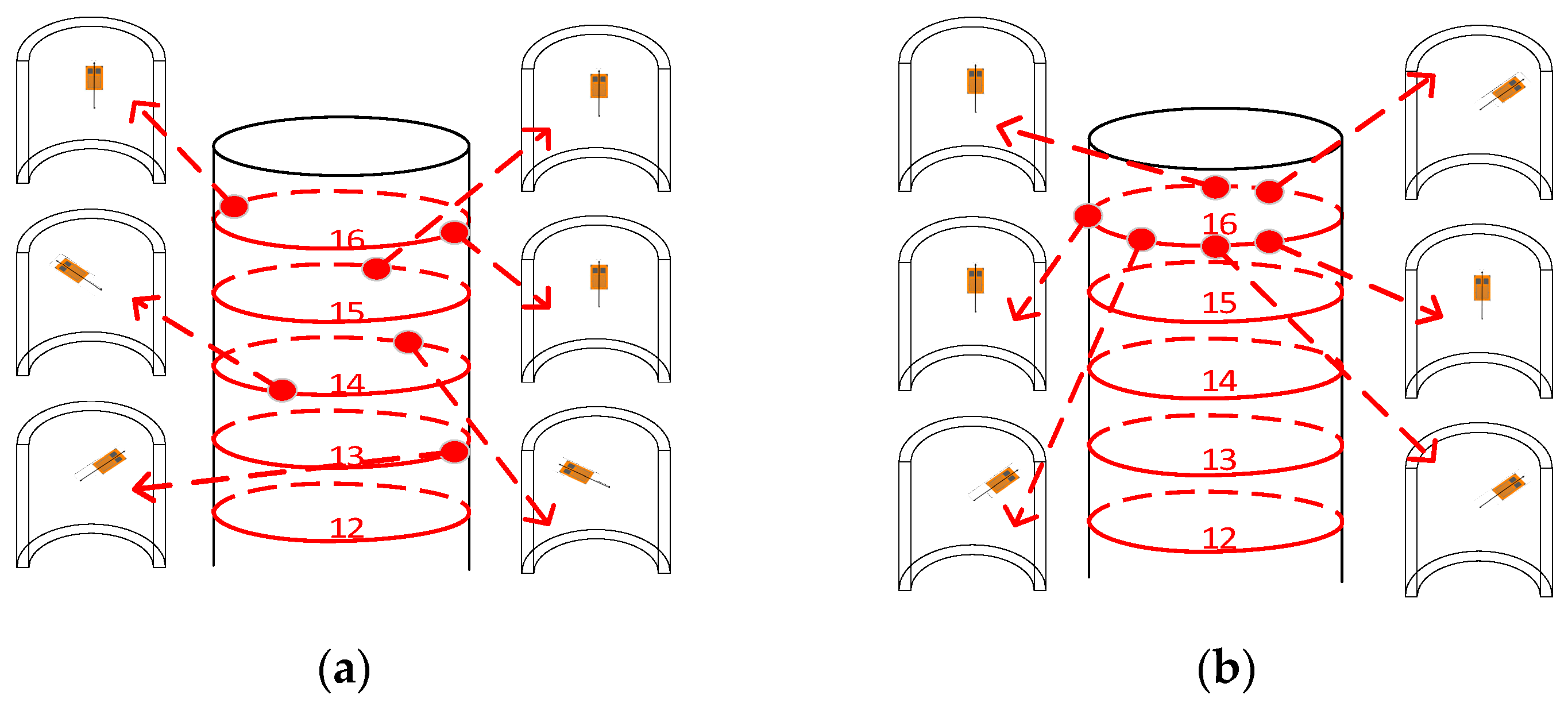
Compare matrix H p × m with matrix H n × m to determine the final measurement point location. The final locations of the measurement points are shown in Figure 15b.
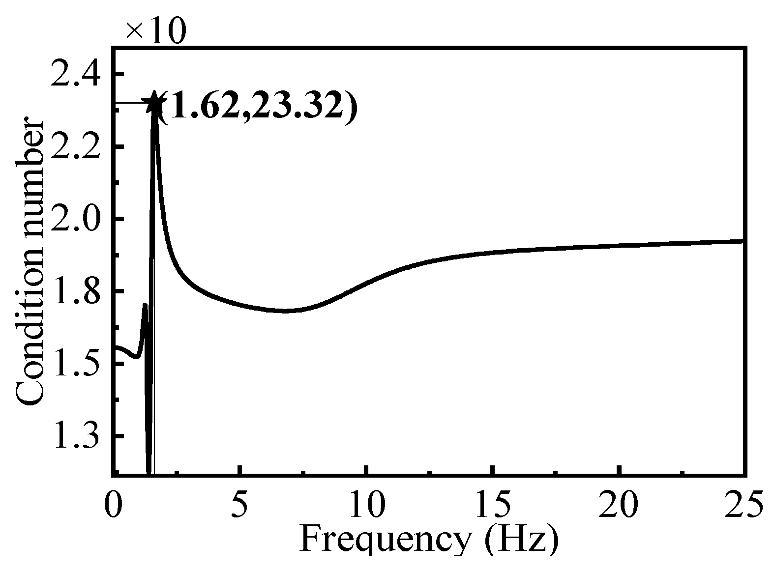
The variation of the condition number of the optimised frequency response function matrix with frequency is illustrated in Figure 16. The maximum condition number of the matrix optimised by the COD method is 23.32, which represents a significant reduction of 486.26 from the condition number of the unoptimised matrix. This substantial decrease highlights the COD method’s effectiveness in reducing the condition number of the frequency response function matrix, playing a pivotal role in optimising sensor placements. The reduced condition number indicates improved numerical stability and potential for more accurate inversion results, which is crucial for reliable load identification.
The wind load spectrum identification mathematical model, constructed using the optimised frequency response function matrix and the corresponding structural response spectrum matrix, is presented in Equation (24). This model integrates the enhancements achieved through the COD method, aiming to provide a more robust framework for accurately determining wind loads based on optimised sensor data.
S y 6 y 6 = H y 6 x 6 × S x x × H y 6 x 6 H
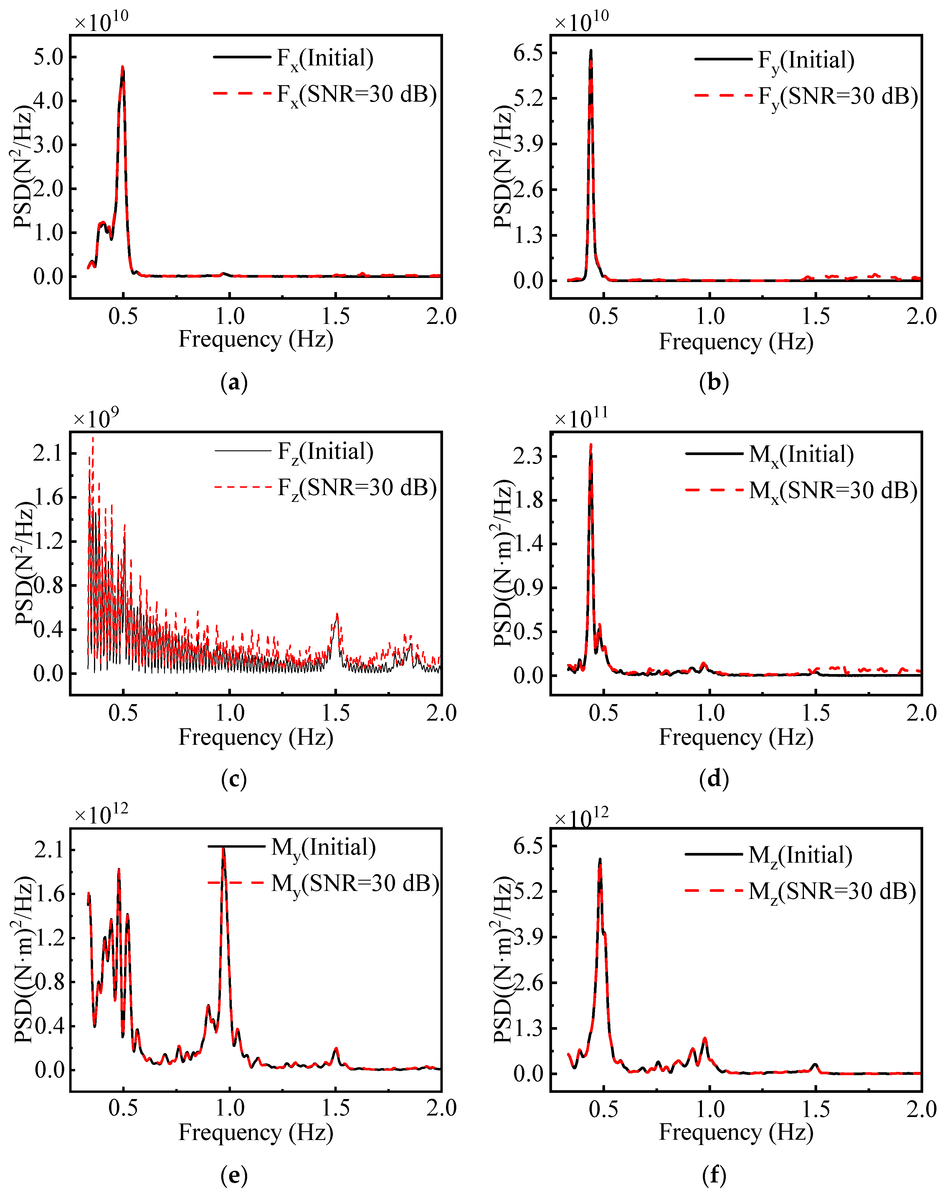
The Moore–Penrose pseudo-inverse method was used to solve Equation (24), and the load identification results are presented in Figure 17.
In the F x , F y , M x , M y , and M z directions, the identified load spectrum largely aligns with the original load spectrum, with a notable exception in the F z direction, where a deviation from the original spectrum was observed. The overall accuracy of the identified wind load spectrum remains high, given the lower magnitude of the load spectrum in the F z direction compared to the other five directions. This high degree of accuracy underscores the efficacy of the optimised sensor placement scheme in precisely identifying the wind load spectrum imposed on the wind turbine tower structure. It also highlights the pivotal role played by the COD method in optimising the sensor arrangement, ensuring that even with a reduced number of sensors, critical load components can be accurately captured.
The DOD method enhances the accuracy of the inverse by maximising | H T n × m × H n × m | through a SEA. In the mathematical model presented in this section, H n × m is a complex matrix, posing a challenge for traditional DOD in efficiently filtering out row vectors in H n × m . Modifying the objective function of DOD to reflect the condition number of the matrix H n × m is imperative to address this limitation [25]. The aim is to minimise the condition number of the matrix H n × m through a SEA, thereby improving the accuracy of load identification. The detailed execution process of DOD is outlined below [22].
(1)
Select the frequency response function matrix corresponding to the peak of the condition number in Figure 13 and randomly select m rows in this frequency response function matrix H n × m to obtain the initial matrix H m × m and the remaining matrix H ( n m ) × m .
(2)
Select a row from the remaining matrix H ( n m ) × m and add it to H m × m to obtain the expanded matrix H ( m + 1 ) × m . There are (n–m) expanded matrices H ( m + 1 ) × m in total.
(3)
Calculate the condition numbers of all the expanded matrices and obtain the expanded matrix H ( m + 1 ) × m corresponding to the minimum condition number.
(4)
Delete one row from the expanded matrix H ( m + 1 ) × m to obtain the original dimension matrix H m × m . There are (m + 1) original dimension matrices H m × m in total.
(5)
Calculate the condition numbers of all the original dimension matrices H m × m to obtain the original dimension matrix H m × m corresponding to the minimum condition number.
(6)
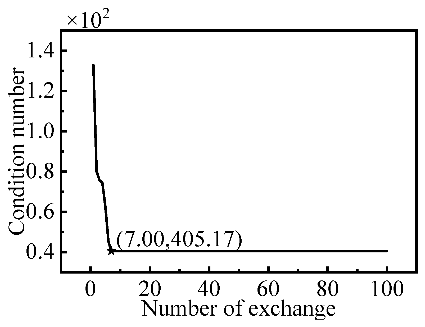
Steps (2)–(4) are the exchanges of measurement point positions. Repeat steps (2)–(4) until the number of conditions is no longer reduced, or the number of sequential exchanges is defined artificially, and the loop is jumped out when the number of runs is achieved. The entire process is shown in Figure 18.
(7)
Compare the final matrix H m × m with the total matrix H n × m to determine the location of the final measurement point. The final location of the measurement point is shown in Figure 15a.
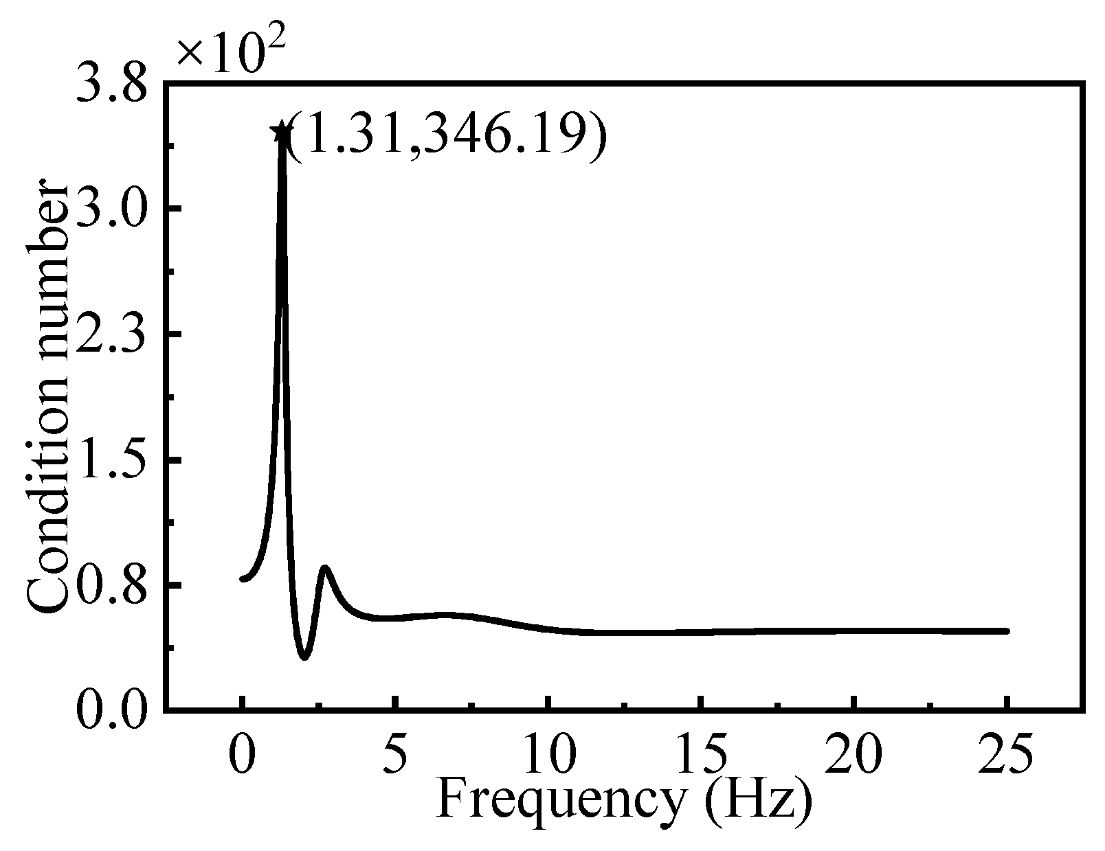
Figure 19 shows how the condition number of the frequency response function matrix, optimised using the DOD method, varies with frequency. From the figure, it can be observed that after optimisation using the DOD method, the maximum condition number of the frequency response function matrix was reduced to 346.19, which is a decrease of 163.39 from the maximum condition number before optimisation. This indicates that the DOD method can optimise the frequency response function matrix to a certain extent; however, the optimisation effect is not as significant as that achieved by the COD method.
The load identification results for the optimised mathematical model using the DOD method were obtained using the Moore–Penrose pseudo-inverse method and are presented in Figure 20.
As illustrated in Figure 20, the DOD method demonstrated satisfactory accuracy in the directions F x , F y , M y , and M z . However, significant discrepancies were observed in the load spectra identified in the F z and M x directions when employing the DOD-optimised mathematical model, exhibiting errors substantially greater than those encountered with the COD method. MAE was adopted as the criterion for evaluating load identification accuracy to facilitate a more rigorous comparison between these two sensor arrangement optimisation algorithms. Table 6 presents the load identification errors both prior to and subsequent to the application of the sensor arrangement optimisation algorithm.
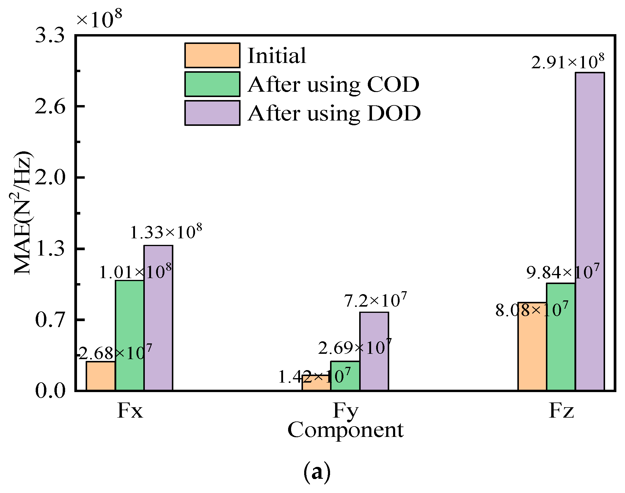
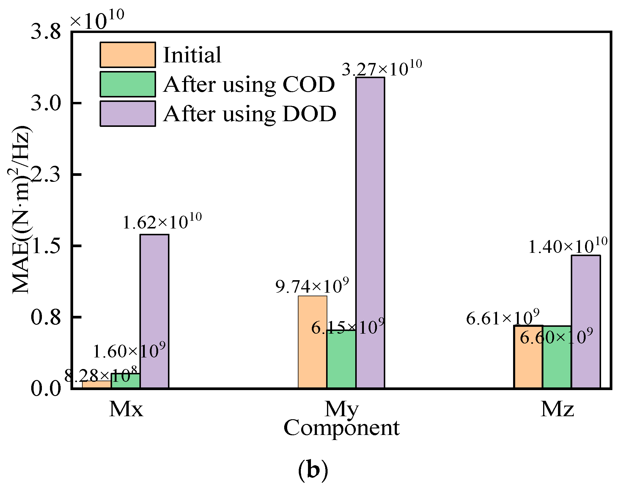
The data in Table 5 and Table 6 are graphically represented as histograms in Figure 21.
As shown in Table 6 and Figure 21, the load identification errors in the directions of F x , F y , F z , and M x increased after optimisation using both the COD and DOD methods. However, the COD method performed better than the DOD method, and the optimised load identification errors were still significantly lower than the peak values of the original load spectra in these four directions. Although the use of the COD method resulted in a slight decrease in load identification accuracy in the directions of F x , F y , F z , and M x , considering the improvement in the identification accuracy in the directions with the highest magnitudes of the original load spectra peaks, M y and M z , the overall load identification accuracy remained at the same level as before optimisation. The DOD method introduced a level of randomness, resulting in different outcomes with each optimisation iteration. The COD method was selected as the sensor placement optimisation algorithm, based on overall performance considerations. Furthermore, the COD method significantly reduced the number of sensors. The initial sensor placement involved 1152 sensors, while the optimised arrangement utilised only 6, and the total number of sensors is 0.5% of the initial number, proving to be very practical for real-world engineering applications.

5. Frequency-Domain Fatigue Analysis

The stress range solution for fatigue calibration is determined based on the hotspot stress. According to specification DNV–OS–J101 [45], the hotspot stress for welded pipe nodes is obtained by extrapolating the first principal stress from the two reference points. In the plane stress state, the first principal stress is calculated using Equation (18):
The power spectrum density function of the stress under wind loading is typically broadband. Approximation methods are commonly employed to calculate fatigue damage, because of the absence of a theoretical solution for the stress range probability density function in broadband spectra. The following methods are predominantly utilised in the domain of ship and ocean engineering.
(1)
The narrowband approximation, which employs Equation (25) for damage calculation, represents a more conservative methodology [46].
D N B = T v 0 C ( 2 2 λ 0 ) m Γ ( m 2 + 1 )
where T is the structural design service life, C and m are S–N curve parameters, v 0 is the average trans-zero rate, λ 0 is the zeroth-order spectral moment of the power spectral density function, and Γ ( ) is the gamma function.
(2)
The bandwidth correction method involves the application of a correction to Equation (27), as expressed in Equation (26)
D W B = ρ W B D N B
where ρ W B is the bandwidth correction factor. The main methods for calculating the bandwidth correction factor ρ W B are the Wirsching–Light [47], Ortiz–Chen [48], and Lutes–Larson methods [49].
(3)
Fatigue damage can be computed using an approximate probability density function formula, widely acknowledged as the Dirlik formula [50].
The semiempirical model devised by Dirlik incorporates a Rayleigh distribution and two exponential distributions. The distribution pattern of this model closely approximates the stress range distribution obtained from rainfall counting. Consequently, this model accurately calculates the fatigue damage caused by broadband stochastic processes. A mathematical representation of the Dirlik model is presented in Equations (27) and (28) with stress ranges following the Dirlik distribution, as shown in Equation (29).
D D i r l i k = v p T C 0 [ S m p R F C D K ( S ) ] d S
D = 0 [ S m p R F C D K ( S ) ] d S
p R F C D K ( S ) = 1 ( λ 0 ) 1 2 G 1 Q e x p ( z Q ) + G 2 z R 2 e x p ( z 2 2 R 2 ) + G 3 z e x p ( z 2 2 )
Based on the DNV GL standard [51], this study determined the parameters for the S-N curve used in the Dirlik formula. The fatigue damage values for six monitoring nodes, as shown in Figure 2, were calculated based on the designed service life of offshore wind turbines being 25 years, with the results presented in Table 7. The fatigue life calculations in the second column are based on structural response spectra obtained from finite element analysis. The structural response spectra were deduced in reverse by applying the load spectra obtained through the load identification method to Equation (1). The fatigue damage values for the six nodes were further calculated based on these response spectra, as shown in the third column of Table 7. A comparison of the data in Table 7 reveals that the relative error between the fatigue damage values calculated based on the identified load spectra and those obtained from finite element simulation response spectra is controlled within 1.5%. This outcome verifies the high accuracy of the identified load spectra, proving its applicability for fatigue damage assessment in engineering analysis.

6. Algorithm Validation

Section 3.2’s analysis establishes that wind speeds in the designated marine area typically range from 8 m/s to 12 m/s, with extremes up to 24 m/s. This section includes numerical examples for wind speeds of 10 m/s, 12 m/s, and the extreme 24 m/s to validate the effectiveness of the proposed model in identifying wind loads atop the jacket wind turbine tower. The analysis in Section 4 reveals that sensor placements at the upper part of the tower, which are optimised through an algorithm, aim to minimize interference from wind loads on structural response measurements as much as possible. The SNR at the tower top under a 12 m/s wind condition is approximately 50 dB, as noted in Section 3.3. For all conditions, 30 dB of Gaussian white noise has been added to the structural response data to replicate actual measurement noise disturbances.

6.1. Identification of Wind Loads at a Wind Speed of 10 m/s

Wind load data at a wind speed of 10 m/s was initially generated using the GH Bladed software, following the procedures detailed in Section 3.5 and Section 4. Subsequently, a mathematical model for wind load identification was established based on this wind speed condition. The COD method was employed to perform dimensionality reduction on the original mathematical model, enhancing the computational efficiency and solution accuracy. The reduced model was then solved using the Moore–Penrose pseudo-inverse method. Figure 22 presents a comparative plot of the wind load identification results, aimed at validating the accuracy and reliability of the proposed method.
The MAE of this load identification is shown in Table 8.
The analysis of Figure 22 and Table 8 reveals that in the directions of F x and F y , where the magnitude of the original load spectrum peaks is approximately 1 0 10 , the magnitude of identified load spectrum errors is about 1 0 8 , significantly lower than the original peaks, indicating a high accuracy in load identification for F x and F y directions. In contrast, for the F z direction, despite the original load spectrum peak being at the magnitude of 1 0 9 , the identification error escalated to 1 0 8 , indicating a reduced accuracy in load identification. For the directions of M x , M y , and M z , with the original load spectrum peaks ranging between 1 0 11 to 1 0 13 in magnitude, the identification errors remained at 1 0 9 , demonstrating high precision in load identification for these directions. Overall, despite the reduced accuracy of the F z direction, the high precision of the M y and M z directions compensates for this inadequacy, validating the effectiveness of the proposed wind load spectrum identification method at a wind speed of 10 m/s in a comprehensive manner.
The calculated structural fatigue damage values from Section 5 are shown in Table 9.
The data in Table 9 show that the fatigue damage estimates obtained through the load identification method closely align with those calculated from structural response spectra derived from finite element simulation, exhibiting a maximum error of only 3.3%. Such a level of error is entirely acceptable within the context of engineering applications. This finding further substantiates the accuracy and reliability of the wind load identification technique proposed in this study, especially under wind speed conditions of 10 m/s.

6.2. Identification of Wind Loads at a Wind Speed of 12 m/s

This example employed GH Bladed to simulate a wind speed of 12 m/s. A mathematical model was constructed for frequency-domain random load identification, and the results were analysed accordingly. A comparative plot of the load identification outcomes is shown in Figure 23.
Table 10 presents the MAE of the load identification.
According to Figure 23 and Table 10, in the directions of F x and F y , the magnitude of the peak areas in the original load spectra is approximately 1 0 10 , while the magnitude of the errors in the identified load spectra is about 1 0 8 , significantly lower than the original peaks, indicating a high level of accuracy in load identification for these directions. In contrast, for the F z direction, with the original load spectrum peak at 1 0 9 , the identification error increased to 1 0 8 , demonstrating a lower accuracy in load identification. For the M x direction, the magnitude of the original load spectrum peak is 1 0 11 , but the identification error is only 1 0 9 , and, combined with Figure 23d, this suggests a moderate accuracy in load identification for the M x direction. In the M y and M z directions, the magnitude of the original load spectrum peaks is 1 0 12 , but the identification error is merely 1 0 9 , indicating a high accuracy in load identification for these directions. Overall, despite the lesser accuracy of the F z direction, the high precision of the M y and M z directions compensates for this inadequacy, validating the overall effectiveness of the proposed method in wind load spectrum identification under wind speeds of 12 m/s.
The fatigue damage values calculated from the identified load spectra are presented in Table 11.
Table 11 reveals that the fatigue damage values calculated using the identified wind load spectra are highly accurate, closely aligning with the fatigue damage values computed based on simulation experiments, with a maximum relative error of 1.8%. This indirectly indicates the high accuracy of the identified load spectra, further substantiating the feasibility and precision of the wind load spectrum identification method proposed in this study.

6.3. Identification of Wind Loads at a Wind Speed of 24 m/s

The maximum wind speed recorded in the region reaches 24 m/s, as indicated by the joint probability distribution of wind and waves presented in Figure A1.
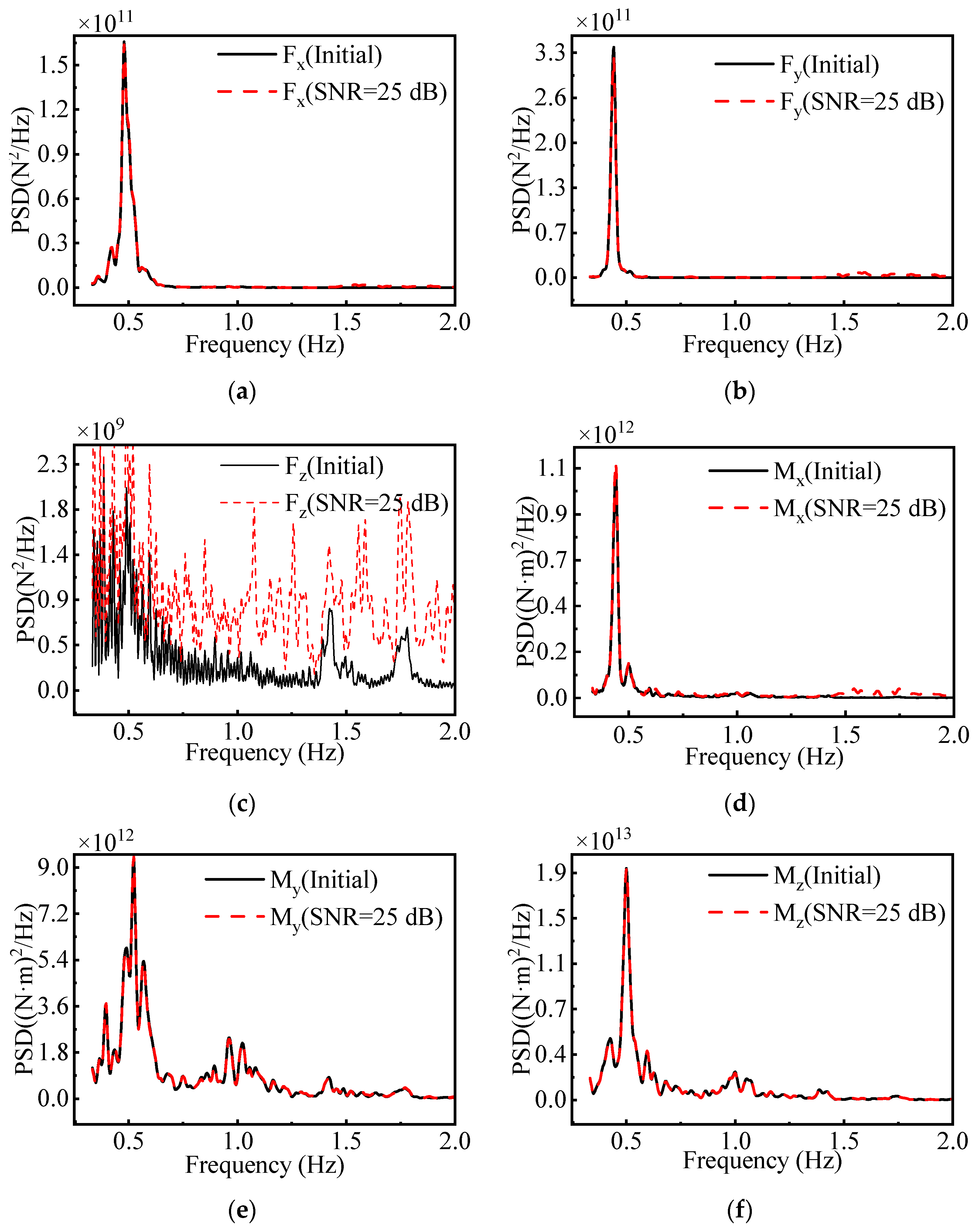
Wind load identification at a wind speed of 24 m/s is conducted to test the established mathematical model’s feasibility and accuracy under extreme conditions. An addition of 25 dB Gaussian white noise to the structure response data is proposed to enhance realism, given the increased disturbance to sensors under extreme conditions. The other settings are similar for wind speeds of 8 m/s, 10 m/s, and 12 m/s. The results of the load identification are presented in Figure 24.
Table 12 presents the MAE of the load identification.
From Figure 24 and Table 12, it is observed that in the directions of F x and F y , the magnitude of the peak areas in the original load spectra is approximately 1 0 11 , while the magnitude of the errors in the identified load spectra ranges between 1 0 8 and 1 0 9 , significantly lower than the original peaks, indicating high accuracy in load spectrum identification for these directions. However, in the F z direction, the identified load spectrum significantly deviates from the original load spectrum, with an identification error magnitude reaching 1 0 8 , closely approaching the magnitude of the original load spectrum peaks, suggesting a low accuracy in load identification for this direction. In the directions of M x , M y , and M z , the magnitude of the identification errors is 2 to 3 orders of magnitude lower than that of the original load spectrum peaks, indicating a high accuracy in load spectrum identification for these directions. Similar to the results analysed for wind speeds of 8 m/s, 10 m/s, and 12 m/s, the accuracy of load identification in the F z direction is relatively lower. However, considering that the magnitude of the load spectrum in the F z direction is inherently the lowest, it can be concluded that the identified wind load spectrum, overall, possesses a commendable level of accuracy.
The fatigue damage values calculated from the identified load spectra are presented in Table 13.
According to the data presented in Table 13, the fatigue damage values calculated using the identified wind load spectra are slightly higher than those obtained through finite element simulation, with the maximum error reaching 5.7%. In comparison, the maximum error in fatigue damage calculations under wind speeds of 8 m/s, 10 m/s, and 12 m/s is approximately 2%, indicating a significant increase in error under the condition of a 24 m/s wind speed. This suggests a reduction in the accuracy of wind load identification at a wind speed of 24 m/s. However, such an error level remains within the acceptable range for practical engineering applications. Moreover, the fact that the fatigue damage values calculated based on the identified wind load spectra are higher than those derived from finite element simulation data represents a conservative approach, aligning with the requirements for addressing engineering problems.

7. Conclusions

The wind load of a wind turbine is usually determined by the statistical parameters of wind speed in the nearby sea area in the design stage of the offshore wind turbine tower. However, the pre-estimated load is different from the actual load encountered by the wind turbine, which leads to uncertainty in the safety of the wind turbine structure. A wind load identification method was developed in this study to accurately obtain the actual wind load encountered by the wind turbine, in which the wind loads are estimated with the input of structural strain response. This is an indirect monitoring method for wind loads. This study utilises the dynamic load identification theory in frequency to reconstruct the PSD of equivalent concentrated wind loads. The candidate strain gauge locations and directions were optimised using DOD and COD algorithms, and then the optimised mathematical model can be obtained and used for PSD reconstruction. Four numerical examples of wind load identification were performed, and the following conclusions can be made.
The wind load identified through the initial mathematical model has excellent accuracy, but a large number of strain gauges is not favourable for practical application. The DOD and COD algorithms can provide optimal mathematical models for the identification of wind loads by optimising strain gauge locations and directions, in which the optimal mathematical model derived from the COD algorithm is better than that derived from the DOD algorithm with the index of the condition number. The identification accuracy of the mathematical model derived from the COD algorithm is better than that of the mathematical model derived from the DOD algorithm. The structural fatigue damage corresponding to the identified wind loads closely approximates that derived from finite element simulation wind loads, with a relative error within 6%.
This study has its limitations. It assumes the frequency response function matrix to be error-free, overlooking potential variations in the system’s frequency response due to changes in material parameters, a condition that may not hold true in practice. While this study has been validated at a theoretical level, its application in real-world engineering projects may require further adjustments and validation. Future research should focus on addressing the uncertainties of the frequency response function matrix, exploring more flexible and accurate models to adapt to the complexities encountered in practical applications.

Author Contributions

F.Z.: conceptualisation, methodology, software, formal analysis, writing—original draft, and validation; M.Z.: resources, project administration, funding acquisition, and writing—review and editing; F.M.: data curation and visualisation; Z.L.: investigation and writing—review and editing; X.Q.: supervision and writing—review and editing. All authors have read and agreed to the published version of the manuscript.

Funding

This work was sponsored and supported by the National Natural Science Foundation of China (52301365), the Natural Science Fund project of Shandong province (ZR2022QE106), the Natural Science Fund project of Heilongjiang province (LH2023E075), the Science and Technology Plan Project of Yantai City (2023JMRH004), the Leading Innovation Project of China National Nuclear Corporation (KY90200220002), and the Special fund for Taishan Industrial Leading Talent Project.

Institutional Review Board Statement

Not applicable.

Informed Consent Statement

Not applicable.

Data Availability Statement

Data are contained within the article.

Conflicts of Interest

The authors declare no conflicts of interest.

Nomenclature

F x The force in the X-direction
F y The force in the Y-direction
F z The force in the Z-direction
M x The moment in the X-direction
M y The moment in the Y-direction
M z The moment in the Z-direction
H Frequency response function matrix
H The superscript denotes the conjugate transpose
S x x Excitation PSD matrix
S y y Response PSD matrix
λ Eigenvalue
φ Eigenvector
r Pseudo-response vector
l Pseudo-excitation vector
e i ω t Unit harmonic excitation
+ The superscript denotes generalised inversion
e r r Error in the response data
U Left singular vector matrix
V Right singular vector matrix
I Identity matrix
S Singular value matrix
Matrix norm
Det ( ) Determinant of a matrix
T The superscript denotes transpose
α The regularisation parameter
σ x Stress in the X-direction
σ y Stress in the Y-direction
τ x y Shear stress
σ 1 First principal stress
σ 3 Third principal stress
α 0 Angle between the direction of the principal stress and the x-axis
U Mean wind speed
u Friction velocity
k Karman constant
D Fatigue damage value
λ 0 Zeroth-order spectral moment
C Parameters of the S-N curve
m Parameters of the S-N curve
ρ W B Bandwidth correction factor
v Average number of cycles per unit time
Φ latitude
S u horizontal wind speed power spectrum
σ u horizontal pulsating wind speed root variance
z 0 ground roughness length
z g gradient height
f c Coriolis constant

Appendix A

Figure A1. Joint probability distribution of wind and waves.
Jmse 12 00563 g0a1

References

  1. Kappel, J.; Wiemann, M.; Kasgen, J.; Jackel, M.; Maetz, T.; Moll, J.; Huhn, H.; Kraemer, P. Development and Installation of a Robust and Reliable Research Structural Health Monitoring System for Grouted Joints of Offshore Wind Turbines. In Proceedings of the the 14th International Workshop on Structural Health Monitoring, Stanford, CA, USA, 12–14 September 2023; Destech Publications, Inc.: Lancaster, PA, USA. [Google Scholar]
  2. Zhang, J.; Li, J. Hybrid Deloading Control Strategy in MMC-Based Wind Energy Conversion Systems for Enhanced Frequency Regulation. Energies 2024, 17, 1253. [Google Scholar] [CrossRef]
  3. Sun, Y.; Luo, L.; Chen, K.; Qin, X.; Zhang, Q. A Time-Domain Method for Load Identification Using Moving Weighted Least Square Technique. Comput. Struct. 2020, 234, 106254. [Google Scholar] [CrossRef]
  4. Wang, C.; Chen, D.; Chen, J.; Lai, X.; He, T. Deep Regression Adaptation Networks with Model-Based Transfer Learning for Dynamic Load Identification in the Frequency Domain. Eng. Appl. Artif. Intell. 2021, 102, 104244. [Google Scholar] [CrossRef]
  5. Bartlett, F.D.; Flannelly, W.G. Model Verification of Force Determination for Measuring Vibratory Loads. J. Am. Helicopter Soc. 1979, 24, 10–18. [Google Scholar] [CrossRef]
  6. Faridi, M.A.; Kuncham, E.; Roy, K.; Singhal, V. Using Limited Roving Sensors to Monitor Bridge Subjected to Random Traffic Load. J. Civ. Struct. Health Monit. 2024, 1–18. [Google Scholar] [CrossRef]
  7. Wu, C.; Jiang, R.; Wu, X.; Zhong, C.; Huang, C. A Time–Frequency Residual Convolution Neural Network for the Fault Diagnosis of Rolling Bearings. Processes 2023, 12, 54. [Google Scholar] [CrossRef]
  8. He, Z.C.; Zhang, Z.; Li, E. Multi-Source Random Excitation Identification for Stochastic Structures Based on Matrix Perturbation and Modified Regularization Method. Mech. Syst. Signal Process. 2019, 119, 266–292. [Google Scholar] [CrossRef]
  9. Liu, Y.; Wang, L. A Two-Step Weighting Regularization Method for Stochastic Excitation Identification under Multi-Source Uncertainties Based on Response Superposition-Decomposition Principle. Mech. Syst. Signal Process. 2023, 182, 109565. [Google Scholar] [CrossRef]
  10. Kong, S.; Cui, H.; Tian, Y.; Ji, S. Identification of Ice Loads on Shell Structure of Ice-Going Vessel with Green Kernel and Regularization Method. Mar. Struct. 2020, 74, 102820. [Google Scholar] [CrossRef]
  11. Liu, J.; Li, K. Sparse Identification of Time-Space Coupled Distributed Dynamic Load. Mech. Syst. Signal Process. 2021, 148, 107177. [Google Scholar] [CrossRef]
  12. Wang, L.; Xu, H.; Liu, Y. A Novel Dynamic Load Identification Approach for Multi-Source Uncertain Structures Based on the Set-Theoretical Wavelet Transform and Layered Noise Reduction. Structures 2023, 51, 91–104. [Google Scholar] [CrossRef]
  13. Guo, L.; Wang, S.; Chen, H.; Shi, Q. A Load Identification Method Based on Active Deep Learning and Discrete Wavelet Transform. IEEE Access 2020, 8, 113932–113942. [Google Scholar] [CrossRef]
  14. Baek, S.-M.; Park, J.-C.; Jung, H.-J. Impact Load Identification Method Based on Artificial Neural Network for Submerged Floating Tunnel under Collision. Ocean Eng. 2023, 286, 115641. [Google Scholar] [CrossRef]
  15. Mao, B.Y.; Xie, S.L.; Xu, M.L.; Zhang, X.N.; Zhang, G.H. Simulated and Experimental Studies on Identification of Impact Load with the Transient Statistical Energy Analysis Method. Mech. Syst. Signal Process. 2014, 46, 307–324. [Google Scholar] [CrossRef]
  16. Jiang, J.; Tang, H.; Mohamed, M.S.; Luo, S.; Chen, J. Augmented Tikhonov Regularization Method for Dynamic Load Identification. Appl. Sci. 2020, 10, 6348. [Google Scholar] [CrossRef]
  17. Zhang, C.; Xu, Y. Comparative Studies on Damage Identification with Tikhonov Regularization and Sparse Regularization. Struct. Control Health Monit. 2016, 23, 560–579. [Google Scholar] [CrossRef]
  18. Chen, T.; Kusche, J.; Shen, Y.; Chen, Q. A Combined Use of TSVD and Tikhonov Regularization for Mass Flux Solution in Tibetan Plateau. Remote Sens. 2020, 12, 2045. [Google Scholar] [CrossRef]
  19. Tian, B.; Ren, H.; Yi, X.; Du, G.; Jiang, C. Noise Suppression Method for Magnetic Resonance Sounding Signals Based on Double Singular Value Decomposition. Radio Sci. 2019, 54, 517–530. [Google Scholar] [CrossRef]
  20. Wang, L.; Han, X.; Liu, J.; Chen, J. An Improved Iteration Regularization Method and Application to Reconstruction of Dynamic Loads on a Plate. J. Comput. Appl. Math. 2011, 235, 4083–4094. [Google Scholar] [CrossRef]
  21. Yue, X.; Jian, C.; Jiazhu, L. A Joint Method of Denoising Correction and Regularization Preconditioned Iteration for Dynamic Load Identification in Time Domain. J. Vib. Eng. 2013, 26, 854–862. [Google Scholar]
  22. Gupta, D.K.; Dhingra, A.K. Input Load Identification from Optimally Placed Strain Gages Using D-Optimal Design and Model Reduction. Mech. Syst. Signal Process. 2013, 40, 556–570. [Google Scholar] [CrossRef]
  23. Zhang, M.; Qiu, B.; Zhu, M.; Qu, X. Novel Computation Method of Reducing Ill-Posedness for Structural Static Distributed Load Identification by Optimising Strain Gauge Locations. Mech. Syst. Signal Process. 2019, 124, 83–110. [Google Scholar] [CrossRef]
  24. Zhang, M.; Qiu, B.; Wei, Q.; Qu, X.; Shi, D. Indirect Ice Load Monitoring and Strength Analysis of a Steel Gate Considering Uncertainties. Measurement 2019, 148, 106919. [Google Scholar] [CrossRef]
  25. Zhang, M.; Qiu, B.; Qu, X.; Shi, D. Improved C-Optimal Design Method for Ice Load Identification by Determining Sensor Locations. Cold Reg. Sci. Technol. 2020, 174, 103027. [Google Scholar] [CrossRef]
  26. Zhang, M.; Qiu, B.; Kalhori, H.; Qu, X. Hybrid Reconstruction Method for Indirect Monitoring of an Ice Load of a Steel Gate in a Cold Region. Cold Reg. Sci. Technol. 2019, 162, 19–34. [Google Scholar] [CrossRef]
  27. Zhang, M.; Sun, L.; Xie, Y. A Monitoring Method of Hull Structural Bending and Torsional Moment. Ocean Eng. 2024, 291, 116344. [Google Scholar] [CrossRef]
  28. Jeong, S.; Kim, E.-J.; Shin, D.H.; Park, J.-W.; Sim, S.-H. Data Fusion-Based Damage Identification for a Monopile Offshore Wind Turbine Structure Using Wireless Smart Sensors. Ocean Eng. 2020, 195, 106728. [Google Scholar] [CrossRef]
  29. Wang, Z.; Qiao, D.; Tang, G.; Wang, B.; Yan, J.; Ou, J. An Identification Method of Floating Wind Turbine Tower Responses Using Deep Learning Technology in the Monitoring System. Ocean Eng. 2022, 261, 112105. [Google Scholar] [CrossRef]
  30. Xu, M.; Au, F.T.K.; Wang, S.; Wang, Z.; Peng, Q.; Tian, H. Dynamic Response Analysis of a Real-World Operating Offshore Wind Turbine under Earthquake Excitations. Ocean Eng. 2022, 266, 112791. [Google Scholar] [CrossRef]
  31. Henderson, A.R. Analysis Tools for Large Floating Offshore Wind Farms; University of London, University College London: London, UK, 2000; ISBN 1-339-31386-3. [Google Scholar]
  32. Wang, L.; Huang, Y.; Xie, Y.; Du, Y. A New Regularization Method for Dynamic Load Identification. Sci. Prog. 2020, 103, 0036850420931283. [Google Scholar] [CrossRef]
  33. Barata, J.C.A.; Hussein, M.S. The Moore–Penrose Pseudoinverse: A Tutorial Review of the Theory. Braz. J. Phys. 2012, 42, 146–165. [Google Scholar] [CrossRef]
  34. Roozbeh, M. Generalized Cross-Validation for Simultaneous Optimization of Tuning Parameters in Ridge Regression. Trans. A Sci. 2020, 44, 473–485. [Google Scholar] [CrossRef]
  35. Pilkey, W.D.; Pilkey, W.D. Formulas for Stress, Strain, and Structural Matrices; John Wiley & Sons: Hoboken, NJ, USA, 2005; Volume 107, ISBN 0-471-52746-7. [Google Scholar]
  36. Mazzaretto, O.M.; Menéndez, M.; Lobeto, H. A Global Evaluation of the JONSWAP Spectra Suitability on Coastal Areas. Ocean Eng. 2022, 266, 112756. [Google Scholar] [CrossRef]
  37. Tamura, Y.; Iwatani, Y.; Hibi, K.; Suda, K.; Nakamura, O.; Maruyama, T.; Ishibashi, R. Profiles of Mean Wind Speeds and Vertical Turbulence Intensities Measured at Seashore and Two Inland Sites Using Doppler Sodars. J. Wind Eng. Ind. Aerodyn. 2007, 95, 411–427. [Google Scholar] [CrossRef]
  38. Choi, E.C. Field Measurement and Experimental Study of Wind Speed Profile during Thunderstorms. J. Wind Eng. Ind. Aerodyn. 2004, 92, 275–290. [Google Scholar] [CrossRef]
  39. Lin, M. Field Measurement of the Natural Wind Characteristics In Coastal Region and Research of Buffeting Response of Long Span Bridge. Ph.D. Thesis, Southwest Jiaotong University, Chengdu, China, 2013. [Google Scholar]
  40. Liu, M.; Liao, H.; Li, M.; Ma, C.; Yu, M. Long-Term Field Measurement and Analysis of the Natural Wind Characteristics at the Site of Xi-Hou-Men Bridge. J. Zhejiang Univ. Sci. A 2012, 13, 197–207. [Google Scholar] [CrossRef]
  41. Luis, A. Spatial and Temporal Coherence via Polarization Mutual Coherence Function. Phys. Scr. 2024, 99, 025501. [Google Scholar] [CrossRef]
  42. Jiang, J.; Ding, M.; Li, J. A Novel Time-Domain Dynamic Load Identification Numerical Algorithm for Continuous Systems. Mech. Syst. Signal Process. 2021, 160, 107881. [Google Scholar] [CrossRef]
  43. Tipu, R.K.; Batra, V.; Suman; Pandya, K.S.; Panchal, V.R. Enhancing Load Capacity Prediction of Column Using eReLU-Activated BPNN Model. Structures 2023, 58, 105600. [Google Scholar] [CrossRef]
  44. Li, Z.; Zhang, M. A Reconstruction Method for Structural Stress Distribution of Wind Turbine Tower Using Optimised Mathematical Model. Ocean Eng. 2024, 301, 117562. [Google Scholar] [CrossRef]
  45. Veritas, D.N. Design of Offshore Wind Turbine Structure. Offshore Stand. DNV-OS-J101 2004, 162–163. [Google Scholar]
  46. Veritas, D.N. Recommended Practice–Riser Fatigue; DNV-RP-F204; DNV: Høvik, Norway, 2004; p. 28. [Google Scholar]
  47. Wirsching, P.H.; Light, M.C. Fatigue under Wide Band Random Stresses. J. Struct. Div. 1980, 106, 1593–1607. [Google Scholar] [CrossRef]
  48. Ortiz, K.; Chen, N.K. Fatigue Damage Prediction for Stationary Wideband Processes. In Proceedings of the Fifth International Conference on Applications of Statistics and Probability in Soil and Structural Engeenering, Vancouver, BC, Canada, 25–29 May 1987. [Google Scholar]
  49. Lutes, L.D.; Larsen, C.E. Improved Spectral Method for Variable Amplitude Fatigue Prediction. J. Struct. Eng. 1990, 116, 1149–1164. [Google Scholar] [CrossRef]
  50. Dirlik, T. Application of Computers in Fatigue Analysis. Ph.D. Thesis, University of Warwick, Coventry, UK, 1985. [Google Scholar]
  51. Det Norske Veritas. Fatigue Design of Offshore Steel Structures; DNVGL-RP-C203; DNV: Bærum, Norway, 2004; p. 23. [Google Scholar]
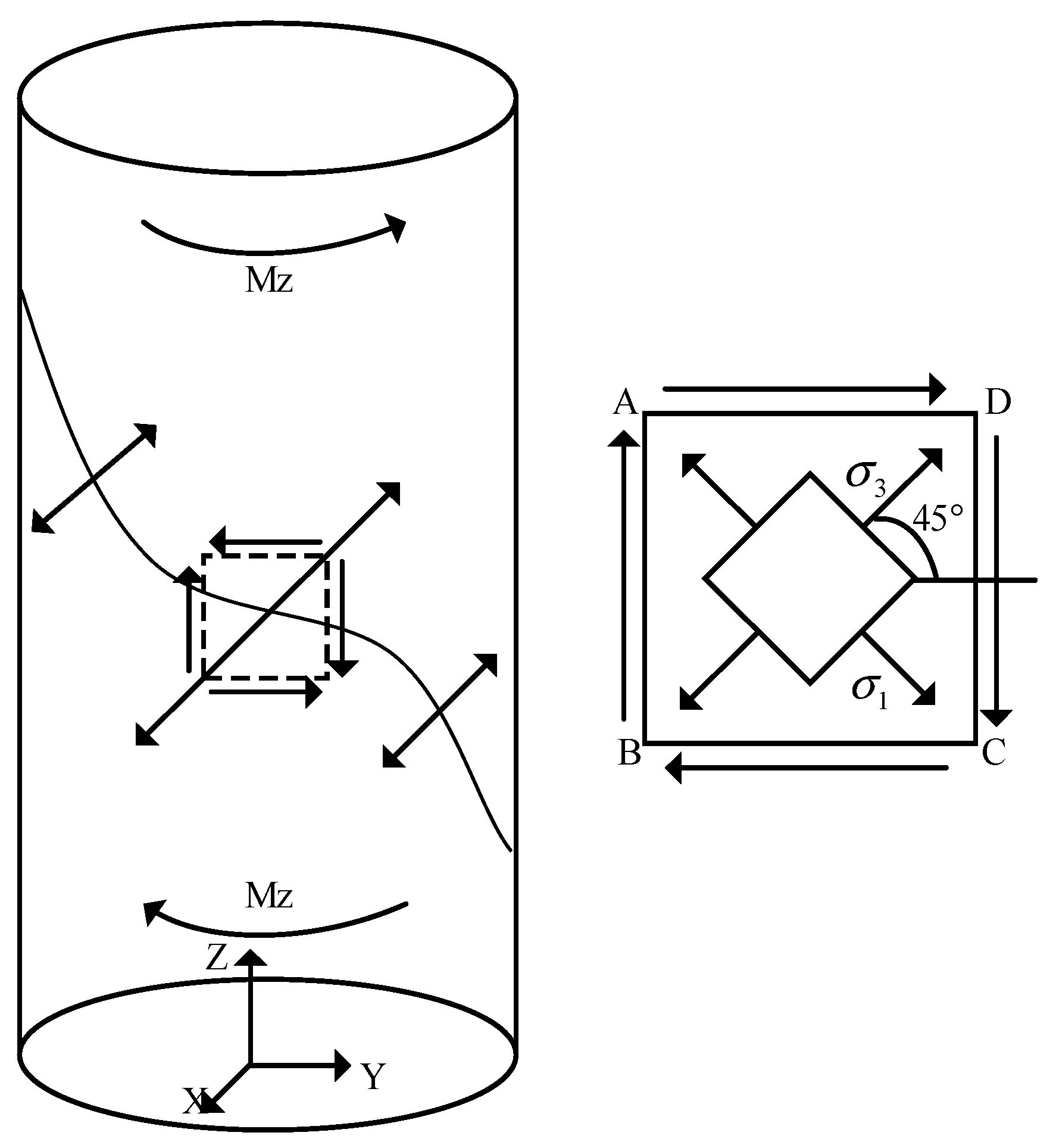
Figure 1. Stress distribution of a cylinder under a bending moment.
Jmse 12 00563 g001
Figure 2. Layout of sensors on the tower structure. (a) Sensor arrangement along the height direction; (b) sensor arrangement in the circumferential direction; (c) sensor arrangement on the inner wall of towers.
Jmse 12 00563 g002
Figure 3. Finite element model of an offshore wind turbine structure.
Jmse 12 00563 g003
Figure 4. Strain range of nodes on the tower drum. (a) First principal strain versus time curve at Node A; (b) first principal strain versus time curve at Node B; (c) first principal strain versus time curve at Node C; (d) first principal strain versus time curve at Node D; (e) first principal strain versus time curve at Node E; (f) first principal strain versus time curve at Node F.
Jmse 12 00563 g004aJmse 12 00563 g004b
Figure 5. Schematic diagrams of finite volume models in the computational domain. (a) Schematic diagram of the computational domain range; (b) finite volume mesh division within the computational domain; (c) detailed view of finite volume grid in the computational domain; (d) detailed view of finite volume grid in the computational domain.
Jmse 12 00563 g005
Figure 6. Airfoil characteristic curve. (a) No. 1 airfoil characteristic curve, R e = 2 × 1 0 6 ; (b) No. 2 airfoil characteristic curve, R e = 8 × 1 0 6 ; (c) No. 3 airfoil characteristic curve, R e = 8 × 1 0 6 ; (d) No. 4 airfoil characteristic curve, R e = 6 × 1 0 6 .
Jmse 12 00563 g006
Figure 7. Time history of aerodynamic load (wind speed = 8 m/s). (a) Time history of concentrated force at the top of the tower; (b) time history of concentrated moment at the top of the tower.
Jmse 12 00563 g007
Figure 8. Load identification of the TRM + L-curve. (a) Power spectral density curve of original load and identified load in F x direction; (b) power spectral density curve of original load and identified load in F y direction; (c) power spectral density curve of original load and identified load in F z direction; (d) power spectral density curve of original load and identified load in M x direction; (e) power spectral density curve of original load and identified load in M y direction; (f) power spectral density curve of original load and identified load in M z direction.
Jmse 12 00563 g008aJmse 12 00563 g008b
Figure 9. Load identification of TRM + GCV. (a) Power spectral density curve of original load and identified load in F x direction; (b) power spectral density curve of original load and identified load in F y direction; (c) power spectral density curve of original load and identified load in F z direction; (d) power spectral density curve of original load and identified load in M x direction; (e) power spectral density curve of original load and identified load in M y direction; (f) power spectral density curve of original load and identified load in M z direction.
Jmse 12 00563 g009aJmse 12 00563 g009b
Figure 10. Load identification of TSVD+L-curve. (a) Power spectral density curve of original load and identified load in F x direction; (b) power spectral density curve of original load and identified load in F y direction; (c) power spectral density curve of original load and identified load in F z direction; (d) power spectral density curve of original load and identified load in M x direction; (e) power spectral density curve of original load and identified load in M y direction; (f) power spectral density curve of original load and identified load in M z direction.
Jmse 12 00563 g010aJmse 12 00563 g010b
Figure 11. Load identification of TSVD + GCV. (a) Power spectral density curve of original load and identified load in F x direction; (b) power spectral density curve of original load and identified load in F y direction; (c) power spectral density curve of original load and identified load in F z direction; (d) power spectral density curve of original load and identified load in M x direction; (e) power spectral density curve of original load and identified load in M y direction; (f) power spectral density curve of original load and identified load in M z direction.
Jmse 12 00563 g011
Figure 12. Load identification of Moore–Penrose. (a) Power spectral density curve of original load and identified load in F x direction; (b) Power spectral density curve of original load and identified load in F y direction; (c) power spectral density curve of original load and identified load in F z direction; (d) power spectral density curve of original load and identified load in M x direction; (e) power spectral density curve of original load and identified load in M y direction; (f) power spectral density curve of original load and identified load in M z direction.
Jmse 12 00563 g012
Figure 13. Change in the condition number of the initial frequency response function matrix.
Jmse 12 00563 g013
Figure 14. Execution process of C-optimal design.
Jmse 12 00563 g014
Figure 15. Optimised measurement point position. (a) Optimised sensor placement by the D-optimal design; (b) optimised sensor placement by the C-optimal design.
Jmse 12 00563 g015
Figure 16. Change in the condition number of the frequency response function matrix after C-optimal design.
Jmse 12 00563 g016
Figure 17. Load identification for C-optimal design. (a) Power spectral density curve of original load and identified load in F x direction; (b) power spectral density curve of original load and identified load in F y direction; (c) power spectral density curve of original load and identified load in F z direction; (d) power spectral density curve of original load and identified load in M x direction; (e) power spectral density curve of original load and identified load in M y direction; (f) power spectral density curve of original load and identified load in M z direction.
Jmse 12 00563 g017
Figure 18. Execution process of D-optimal design.
Jmse 12 00563 g018
Figure 19. Change in the condition number of the frequency response function matrix after D-optimal design.
Jmse 12 00563 g019
Figure 20. Load identification for DOD. (a) Power spectral density curve of original load and identified load in F x direction; (b) power spectral density curve of original load and identified load in F y direction; (c) power spectral density curve of original load and identified load in F z direction; (d) power spectral density curve of original load and identified load in M x direction; (e) power spectral density curve of original load and identified load in M y direction; (f) power spectral density curve of original load and identified load in M z direction.
Jmse 12 00563 g020
Figure 21. Comparison of load identification errors before and after sensor arrangement optimisation. (a) Comparison of mean absolute error values for load identification in the F x , F y , and F z directions without sensor optimisation, C-optimal design optimisation, and D-optimal design optimisation. (b) Comparison of mean absolute error values for load identification in the M x , M y , and M z directions without sensor optimisation, C-optimal design optimisation, and D-optimal design optimisation.
Jmse 12 00563 g021aJmse 12 00563 g021b
Figure 22. Load identification at a wind speed of 10 m/s. (a) Power spectral density curve of original load and identified load in F x direction; (b) power spectral density curve of original load and identified load in F y direction; (c) power spectral density curve of original load and identified load in F z direction; (d) power spectral density curve of original load and identified load in M x direction; (e) power spectral density curve of original load and identified load in M y direction; (f) power spectral density curve of original load and identified load in M z direction.
Jmse 12 00563 g022
Figure 23. Load identification at a wind speed of 12 m/s. (a) Power spectral density curve of original load and identified load in F x direction; (b) power spectral density curve of original load and identified load in F y direction; (c) power spectral density curve of original load and identified load in F z direction; (d) power spectral density curve of original load and identified load in M x direction; (e) power spectral density curve of original load and identified load in M y direction; (f) power spectral density curve of original load and identified load in M z direction.
Jmse 12 00563 g023
Figure 24. Load identification at a wind speed of 24 m/s. (a) Power spectral density curve of original load and identified load in F x direction; (b) power spectral density curve of original load and identified load in F y direction; (c) power spectral density curve of original load and identified load in F z direction; (d) power spectral density curve of original load and identified load in M x direction; (e) power spectral density curve of original load and identified load in M y direction; (f) power spectral density curve of original load and identified load in M z direction.
Jmse 12 00563 g024
Table 1. Signal-to-noise ratio of six nodes.
Node NumberSNR (dB)SNR (dB)SNR (dB)
Node 139.092038.828439.9995
Node 252.205737.070932.1821
Node 352.751637.708633.5127
Node 450.922636.714532.8440
Node 550.857938.989135.6809
Node 650.778940.126937.3964
Node 752.407241.672650.6944
Node 852.707633.089144.4267
Node 949.732727.891840.9444
Node 1047.392327.952140.2653
Node 1144.917826.032440.7441
Node 1243.710124.758140.8920
Node 1347.661338.267943.3208
Node 1455.928636.268240.8216
Node 1556.956539.306442.9643
Node 1656.963639.589241.6206
Node 1756.350242.316444.4427
Node 1855.914143.986646.2169
Node 1943.656539.754443.4904
Node 2037.446534.263936.1277
Node 2129.783932.007131.5327
Node 2233.422734.382931.2402
Node 2333.973435.414630.3160
Node 2433.992336.178129.2770
Table 2. Geometric parameters of blades.
Distance from Root
(m)
Chord
(m)
Twist
(deg)
Thickness
(%)
Pitch Axis
(%)
Foil Section
Number
02.902099.9950.001
103.8212.2865.8550.851
204.296.9136.2847.752
303.413.5732.7643.212
402.631.2031.1939.872
502.06−0.4929.6737.283
601.61−1.4326.8336.993
701.17−0.2822.2737.764
78.90.052.5421.0049.204
Table 3. Mass and stiffness parameters of blades.
Distance from Root
(m)
Centre of
Mass (x’)
(%)
Centre of
Mass (y’)
(%)
Mass Axis
Orientation
(deg)
Radius of
Gyration Ratio
00.0050.010.001.00
10−0.0949.7419.350.83
20−0.2847.6510.280.56
30−0.7544.757.440.54
40−0.7942.264.590.50
50−0.8840.202.340.49
600.0940.120.610.45
702.8640.081.290.38
78.92.5349.533.040.20
Table 4. von Karman spectrum calculation parameters.
ParameterValue
Latitude (deg)34
Surface roughness0.01
Average wind speed (m/s)8
Angular velocity of earth’s rotation (rad/s) 7.292 × 10 5
Height of hub centre of wind turbine (m)103
Table 5. Mean absolute error of five solving methods.
ComponentTRM +
L-Curve
TRM +
GCV
TSVD+
L-Curve
TSVD +
GCV
Moore–Penrose
F x ( N 2 / H z )6.60 × 1081.23 × 1086.24 × 1082.12 × 1082.68 × 107
F y ( N 2 / H z )4.91 × 1072.65 × 1078.58 × 1072.24 × 1071.42 × 107
F z ( N 2 / H z )2.09 × 1086.33 × 1079.02 × 1076.46 × 1078.08 × 107
M x ( ( N m ) 2 / H z )8.44 × 1095.01 × 1096.27 × 1092.89 × 1098.28 × 108
M y ( ( N m ) 2 / H z ))3.44 × 10112.16 × 10112.88 × 10112.68 × 10119.74 × 109
M z ( ( N m ) 2 / H z ))4.46 × 10111.17 × 10112.16 × 10111.14 × 10116.61 × 109
Table 6. Mean absolute error of load identification.
ComponentMAE (COD)MAE (DOD)MAE (Initial)
F x ( N 2 / H z )1.01 × 1081.33 × 1082.68 × 107
F y ( N 2 / H z )2.69 × 1077.20 × 1071.42 × 107
F z ( N 2 / H z )9.84 × 1072.91 × 1088.08 × 107
M x ( ( N m ) 2 / H z )1.60 × 1091.62 × 10108.28 × 108
M y ( ( N m ) 2 / H z ))6.15 × 1093.27 × 10109.74 × 109
M z ( ( N m ) 2 / H z ))6.60 × 1091.40 × 10106.61 × 109
Table 7. Comparison of fatigue damage values.
Node NumberFatigue Damage Values Calculated by SimulationFatigue Damage Values Calculated from
Identified Load Spectra
Percentage of
Relative Error
Node A6.37 × 10−46.43 × 10−40.9%
Node B7.17 × 10−47.09 × 10−41.2%
Node C1.87 × 10−51.86 × 10−50.2%
Node D8.26 × 10−48.26 × 10−40.1%
Node E8.63 × 10−48.65 × 10−40.2%
Node F1.00 × 10−39.95 × 10−40.5%
Table 8. MAE of load identification.
ComponentMAE
F x ( N 2 / H z )1.34 × 10⁸
F y ( N 2 / H z )2.99 × 10⁸
F z ( N 2 / H z )1.17 × 10⁸
M x ( ( N m ) 2 / H z )2.27 × 10⁹
M y ( ( N m ) 2 / H z ))7.31 × 10⁹
M z ( ( N m ) 2 / H z ))8.03 × 10⁹
Table 9. Comparison of fatigue damage values.
Node NumberFatigue Damage Values Calculated by SimulationFatigue Damage Values Calculated from
Identified Load Spectra
Percentage of
Relative Error
Node A2.43 × 10−32.51 × 10−33.3%
Node B1.17 × 10−31.15 × 10−31.8%
Node C1.17 × 10−51.17 × 10−50.0%
Node D1.51 × 10−31.51 × 10−30.4%
Node E1.14 × 10−31.14 × 10−30.1%
Node F1.60 × 10−31.58 × 10−31.3%
Table 10. Mean absolute error of load identification.
ComponentMAE
F x ( N 2 / H z )1.41 × 10⁸
F y ( N 2 / H z )3.41 × 10⁸
F z ( N 2 / H z )1.56 × 10⁸
M x ( ( N m ) 2 / H z )2.29 × 10⁹
M y ( ( N m ) 2 / H z ))1.17 × 10¹⁰
M z ( ( N m ) 2 / H z ))1.10 × 10¹⁰
Table 11. Comparison of fatigue damage values.
Node NumberFatigue Damage Values Calculated by SimulationFatigue Damage Values Calculated from
Identified Load Spectra
Percentage of
Relative Error
Node A3.36 × 10−43.39 × 10−40.9%
Node B1.86 × 10−31.83 × 10−31.8%
Node C2.66 × 10−52.66 × 10−50.1%
Node D2.10 × 10−32.10 × 10−30.0%
Node E7.48 × 10−47.48 × 10−40.0%
Node F1.61 × 10−31.59 × 10−31.7%
Table 12. Mean absolute error of load identification.
ComponentMAE
F x ( N 2 / H z )3.40 × 10⁸
F y ( N 2 / H z )1.03 × 10⁹
F z ( N 2 / H z )5.98 × 10⁸
M x ( ( N m ) 2 / H z )6.64 × 10⁹
M y ( ( N m ) 2 / H z ))3.01 × 10¹⁰
M z ( ( N m ) 2 / H z ))3.45 × 10¹⁰
Table 13. Comparison of fatigue damage values.
Node NumberFatigue Damage Values Calculated by SimulationFatigue Damage Values Calculated from
Identified Load Spectra
Percentage of
Relative Error
Node A6.23 × 10−56.59 × 10−55.7%
Node B2.14 × 10−42.26 × 10−44.2%
Node C7.31 × 10−57.68 × 10−55.1%
Node D5.68 × 10−45.74 × 10−41.1%
Node E4.13 × 10−34.29 × 10−33.9%
Node F6.35 × 10−56.68 × 10−55.2%
Disclaimer/Publisher’s Note: The statements, opinions and data contained in all publications are solely those of the individual author(s) and contributor(s) and not of MDPI and/or the editor(s). MDPI and/or the editor(s) disclaim responsibility for any injury to people or property resulting from any ideas, methods, instructions or products referred to in the content.