Abstract
Underwater localization is one of the key techniques for positioning, navigation, timing (PNT) services that could be widely applied in disaster warning, underwater rescues and resource exploration. One of the reasons why it is difficult to achieve accurate positioning for underwater targets is due to the influence of uneven distribution of underwater sound velocity. The current sound-line correction positioning method mainly aims at scenarios with known target depth. However, for nodes that are non-cooperative nodes or lack depth information, sound-line tracking strategies cannot work well due to non-unique positional solutions. To solve this problem, we propose an iterative ray tracing 3D underwater localization (IRTUL) method for stratification compensation. To demonstrate the feasibility of fast stratification compensation, we first derive the signal path as a function of initial |grazing angle, and then prove that the signal propagation time and horizontal propagation distance are monotonic functions of the initial grazing angle, which guarantees the fast achievement of ray tracing. Simulation results indicate that IRTUL has the most significant correction effect in the depth direction, and the average accuracy has been improved by about 3 m compared to a localization model with constant sound velocity.
1. Introduction
Underwater localization is one of the most essential techniques for building marine positioning, navigation and timing (PNT) systems, and could be widely used for disaster warning, underwater rescue and resource exploring. Compared with radio or optical signal, acoustic wave has become the most popular signal carrier in underwater localization [1]. However, unlike terrestrial radio, the acoustic localization faces many challenges due to the special underwater environment, such as the difficulty in clock synchronization [1,2], the multipath effect [3], insufficient reference nodes [3] and the stratification effect [4,5].
Comprehensive surveys of challenges and techniques in localization have been carried out in [1,2,3,4]. Because of the features of underwater acoustic channels, high-precision positioning faces challenges mentioned above. To improve the reliability and accuracy of the positioning, early positioning work mainly focused on the clock asynchronization problem for accurate underwater positioning [6,7,8,9,10]. With the development of urban positioning and indoor wireless positioning technology, many advanced signal processing technologies have emerged to weaken multipath signals or enhance the main path signals, such as sparse channel estimation [11,12], turbo equalization [13,14], decision feedback equalization [15], time reversal mirror in [16], etc. As the scale of underwater networks expands, large-scale positioning has received widespread attention and various methods have been proposed to tackle this problem [17,18,19,20].
The aforementioned methods and algorithms have provided good solutions for dealing with high latency, strong multipath and limited node coverage for positioning. However, they overlooked an important issue, that is, that the non-uniformly distributed underwater sound velocity leads to a significant Snell effect in the signal propagation trajectory [1,2,4]. A strong Snell effect leads to signal propagation path bending, which makes it difficult to accurately measure the signal propagation range. To reduce the accuracy loss of positioning caused by sound velocity estimation error, some works have been carried out to study how to correct the positioning error caused by sound velocity, which is called stratification compensation in this paper.
Diamant and Lampe regard the sound velocity as an invariant parameter to be solved in their proposed localization algorithm [21]. Liu et al. proposed a joint synchronization and localization method in [22] and Zhang et al. combined TDOA and AOA measurements for localization with a constrained weighted least-squares estimator in [23]. Refs. [22,23] addressed the problem of stratification compensation, but mainly focused on system nodes with known target depth information. For detected target nodes or nodes with damaged depth sensor, existing stratification compensation methods are difficult to apply.
In order to accurately locate non-cooperative targets or cooperative targets with damaged depth sensor, we propose a stratification compensation 3D underwater localization method based on iterative ray tracing (IRTUL). The core idea is to optimize the matching degree between simulated sound field and measured sound field based on ray tracing theory, and iteratively correct the target location. To accelerate the positioning algorithm, we derive the signal propagation time and horizontal propagation distance in ray theory as a function of the initial grazing angle, and prove that they are both monotonically related to the initial grazing angle, so that the dichotomy method can be used for rapid searching of sound lines. Meanwhile, we propose a simplified expression method for the SVP, which reduces the sampling points and reduces the computational burden of ray tracing while ensuring the accuracy of signal ray tracing. The contributions of this paper are summarized as follows:
- To accurately localize underwater targets without knowing depth information, we propose an IRTUL method that could accurately locate targets without prior depth information.
- To demonstrate the feasibility of fast ray tracing, we derive the signal path as a function of initial grazing angle, then prove the executability of fast ray tracing.
- To accelerate the ray tracing process, we propose an SVP simplification method, which reduces the computational cost of ray tracing.
The rest of this paper is organized as follows. In Section 2, related works about acoustic localization are reviewed. In Section 3, we propose the IRTUL method for underwater target positioning, conduct some mathematical analyses and present the fast achievement flowchart for IDAUL. Experimental results are discussed in Section 4, and conclusions are given in Section 5.
2. Related Works
Youngberg proposed a buoy-based long baseline positioning system in [24], in which several buoys are used to form a long-baseline underwater acoustic localization system and provide navigation services for underwater users. In 1995, Thomas introduced a GPS-assisted intelligent buoy underwater positioning system. Afterwards, commercial acoustic positioning systems were produced by various companies, such as Kongsberg Simrad in Norway, Link Quest in the United States, Nautronix in Australia and Sonardyne in the United Kingdom.
In order to improve the reliability and real-time performance of acoustic positioning, many terrestrial positioning algorithms have migrated to underwater positioning systems; however, the natural characteristics of underwater environments poses challenges for improving the accuracy and real-time performance of positioning algorithms. Erol et al. conducted research on existing architectures and positioning algorithms in [25], analyzing the differences between acoustic networks and terrestrial internet of things (IoT), as well as the impact of high attenuation, high latency and other special characteristics of the marine environment on underwater positioning. Tan et al. and Luo et al., respectively, analyzed the difficulties and challenges in underwater target positioning in [1,4], and pointed out the main factors affecting positioning accuracy, such as the change of sound velocity, clock asynchrony and movement of sensor nodes.
According to the positioning mode, localization algorithms can be divided into non-ranging and ranging-based positioning algorithms. The non-ranging localization algorithm mainly estimates the approximate position of targets based on the coverage area of reference nodes [26,27,28,29,30,31,32,33]. The non-ranging positioning algorithms have the advantage of low communication energy consumption and long life periods, but with the accuracy performance it is difficult to meet the growing accuracy demand.
For accurate positioning, ranging-based positioning algorithms leveraging sound field observation information such as time of arrival (TOA), time difference of arrival (TDOA), angle of arrival (AOA) and received signal strength indicator (RSSI) have been widely studied. Early positioning algorithms mainly addressed the clock asynchronous problem [6,7,8,9], these positioning algorithms provide excellent solutions for dealing with asynchronous clocks of underwater nodes, but require a certain number of static anchor nodes. The localization of underwater nodes typically requires at least four reference nodes; however, due to the limited communication coverage of reference nodes, there may not be enough reference nodes for some nodes to be located. Many works have been proposed to tackle this problem and solve the problem of large-scale network localization [17,18,34,35,36,37,38,39,40,41,42].
The research works mentioned above provide various solutions for positioning in different scenarios, and combined with advanced signal processing algorithms, the impact of clock asynchronization and limited reference node’s coverage on positioning accuracy can be effectively reduced. However, due to the spatio-temporal variability of underwater sound velocity, there will be obvious stratification effects. Therefore, there may be significant positioning errors when assuming that the signal propagates in a straight line. To tackle this issue, Diamant and Lampe regarded the sound velocity as a parameter to be solved in positioning [21], but the unknown sound velocity is assumed to be invariant, limiting its application scenarios of deep ocean coverage. Ramezani et al. adopted the Time-of-Flight (ToF) measurements in [43] to compensate for the stratification. Based on [43], Liu et al. proposed a joint synchronization and localization method in [22], and Zhang et al. combined TDOA and AOA measurements for localization with a constrained weighted least-squares estimator in [23]. Refs. [22,23,44,45] addressed the problem of stratification compensation, but mainly aimed at system nodes with known target depth information, and their applications are limited for situations where the target depth information is unknown or inaccurate. Gong et al. adopted deep neural networks to detect and locate a mobile underwater target in [46]; however, only average sound speed could be estimated. Inspired by [46], Yan et al. proposed a broad-learning-based localization algorithm with isogradient SVPs in [47], but faced the same problem as [22,23,44,45] when the depth is unknown. The deep-learning-based algorithms in [46,47] have historical memory to update position output, but suffer from a time-consuming training process due to a large number of parameters in filters and layers.
The stratification effect seriously affects the accuracy of underwater localization and has received widespread attention. However, existing works with stratification compensation rely on the depth information measured by depth sensors. When the depth information is unknown or inaccurate, it is a challenge to accurately locate the target.
3. Iterative Ray-Tracing-Based Acoustic Localization for IoUT
3.1. System Model
To solve the multi-solution issue during ray tracing, we propose an IRTUL method, in which the 3D underwater localization problem is separated into multiple 2D localization problems. The localization system construction is shown in Figure 1.
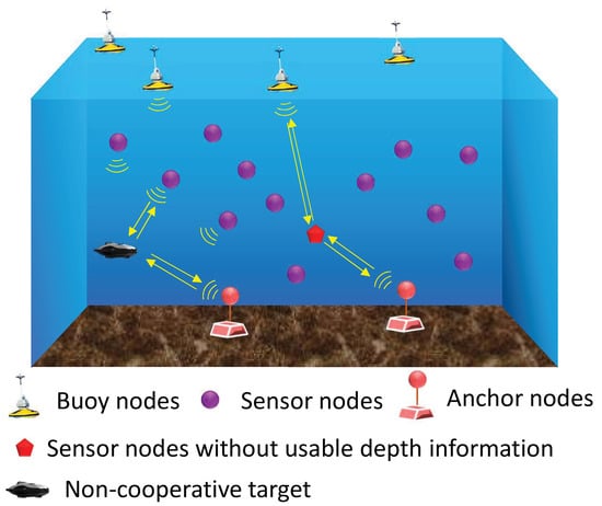
Figure 1.
Localization system for underwater networks.
In this paper, we introduce our positioning method based on underwater networks. The localization network system consists of three types of reference nodes: buoy nodes, sensor nodes and anchor nodes. The position of buoy nodes is obtained via GPS and updated in real time. Anchor nodes are fixed by carrying heavy objects and sinking to the seabed, which only need to be located when they are deployed. Sensor nodes are periodically located with the help of buoy and anchor nodes. There are two kinds of nodes to be located in our system, one is the sensor node whose depth information could not be directly measured through depth sensors, the other is the non-cooperative target whose depth information is an unknown parameter. The sensor node can communicate and interact with the reference node to achieve distance measurement, while non-cooperative targets need to use detection signals for round-trip distance measurement.
There are two stages as shown in Figure 2; one is the sensor positioning stage, during which the sensor target is located, and it can be further divided into location request stage and location response stage. The other is the observation stage, during which the non-cooperative target is located, and it can be further divided into four stages: listening, starting, detecting and collecting. Both the sensor target and the non-cooperative target are located through the round-trip TOA to reduce ranging errors caused by clock asynchronization.
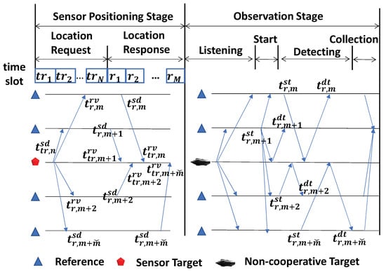
Figure 2.
Positioning stage division.
3.1.1. Sensor Node Localization
During the sensor positioning stage, time division multiplexing is adopted to complete the transmission of messages between nodes by considering the sparse distribution of underwater nodes. During the location request stage, the sensor target node that needs to be located broadcasts the location request information in the preset time slot according to the node number order. Then, in the location response stage, reference nodes also answer the location request in sequence by node number. Once a sensor node is located, it could act as a new reference node. The position of reference nodes floating on the sea or in water will move with the movement of water flow, so in order to reduce the positioning error caused by this, the positioning process needs to be executed periodically. However, within a single positioning cycle, due to a communication time of typically only a few seconds, we ignore the impact of node mobility.
Assume the position of the nth sensor target is , and the position of the mth reference node is . At time , the sensor target node asks for positioning, and its messages arrive at reference node m at time . The single-trip distance observation value will be:
where is the real distance between sensor target n and reference node m, is the ranging error caused by clock asynchronization, is the ranging error caused by using constant sound speed value as 1500 m/s and is the error caused by environmental noise.
Without losing generality, let the reference node answer the location request at time , and the answer message arrive at the sensor target at time , the nth sensor target’s clock lags behind the reference node m with an amount of ; then, the round-trip ranging will be:
Let , ; Equation (2) will be:
where the clock asynchronization error could be eliminated through round-trip TOA.
Because the depth information is not known in this paper, there should be at least four reference nodes to finish the localization. Assume the number of reference nodes that lays within the communication coverage of the sensor target is ; there will be:
where is the estimated location of the sensor target node. The optimization objective of the positioning model will be:
3.1.2. Non-Cooperative Node Localization
During the observation stage, the reference sensor node detects the non-cooperative target through active sonar to eliminate the time synchronization errors. All reference nodes start at the listening stage. Once a random reference node hears the radiated noise, it initiates a detection process as a temporary head node. The head node first sends out a detection signal and uses it to awaken neighboring reference nodes, which respectively send their detection signals for target ranging.
Different from sensor node localization, the detection signals will be immediately returned upon reaching the target surface, so there is no signal processing delay on the target node, and the time asynchronization error could also be eliminated through round-trip transmission similar to Equation (2). Let the th reference node be the head node; the detection signal is sent out at time , and returned at time ; then, the round-trip ranging will be:
where means non-cooperative target.
3.2. IRTUL for Target without Depth Information
For a given SVP , where is the (i + 1)th sampling depth, is the corresponding sound speed value; the signal propagation time and horizontal distance are provided in [48] as:
where is the sound speed value of the first sampling depth, is the initial grazing angle and means the gradient of sound speed of the ith depth layer, which satisfies:
A representative example of signal propagation is shown in Figure 3. Signal propagation has symmetry. When the transmission angle of the reply signal is the same as the arrival angle of the received signal, the signal will return along the original path.
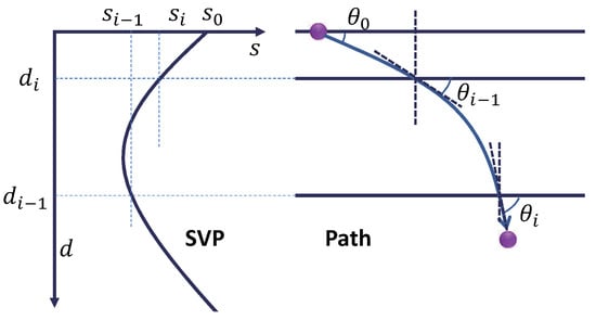
Figure 3.
An example of signal propagation.
According to Snell’s law of refraction:
where is the refractive index at the ith depth layer. There will be:
Considering the trigonometric relationship:
Equations (8) and (9) can be, respectively, derived as:
where ,. Equations (16) and (17) indicate that the signal propagation time and horizontal propagation distance can be expressed as a function of the initial grazing angle. However, the prerequisite is that the depth range of signal propagation is given. When the transmission depth is not prior information, the application of Equations (16) and (17) will be restricted.
To achieve accurate positioning, we propose the IRTUL that is shown in Figure 4. At the beginning, the target node is roughly located as with a linear propagation model based on the average ocean sound speed 1500 m/s. When coming into the bth turn of iteration, based on the current positioning depth of the target node, the first step is to search the initial grazing angle of the signal through Equation (16) that exactly takes time to be transmitted from the reference node to the current target depth. The second step is to calculate the horizontal transmitted distance of the signal through Equation (17). Assume there are reference nodes; then, similar to Equation (4), there will be:
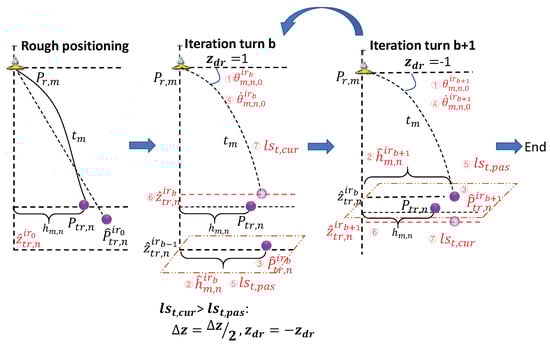
Figure 4.
Scheme of IRTUL.
Subtract the first term from each sub-equation in Equation (18); we can obtain Equations (19) and (20):
where .
where , A and B satisfy:
Equation (20) can be solved through the least square (LS) method:
The third step is to form the position of target node after horizontal distance correction. At the fourth step, the new initial grazing angle is searched according to Equation (17). Then, the signal propagation time before depth tuning is simulated according to (16), and the time lose function is defined by the fifth step as:
where is the measured signal propagation time related to reference node m. At the sixth step, the depth will be adjusted by , where at the beginning. The step size is controlled by , while the direction is controlled by . After depth tuning, the final signal propagation time is simulated again and the final lose function is calculated as:
Through comparison of and , the depth tuning step and direction will be modified. For example, if , it is indicated that the sound field matching error is increased after depth tuning; thus, and . The aforementioned process will continue until , where is a preset threshold.
The position of reference nodes used in Figure 4 is an instantaneous position. Therefore, the positioning result also corresponds to an instantaneous moment position. That is to say, position changes of buoys due to the float of water current will not affect the execution of the positioning algorithm.
3.3. Fast Achievement of Iterative Ray Tracing Localization
The localization approach is based on the iterative idea, so with the computational efficiency it is quite important to achieve real-time positioning. In this section, we first analyze the feasibility of fast ray tracing, then propose the fast IRTUL algorithm and give the computational complexity.
3.3.1. Feasibility Analysis of Fast Ray Tracing
In IRTUL, there are two ways to speed up the algorithm, one is setting the number of SVP depth layers during one ray tracing, and the other is the signal ray searching method.
Simplification of the SVP
According to the derived ray tracing theory Equations (16) and (17), the complexity of calculating signal propagation time and horizontal propagation distance depends on the number of layers in the given SVP. Ray tracing is a model based on linear layering of SVP. Although the actual SVP is non-linear, when high-density sampling is performed on an SVP, the sound speed distribution between sampling points can be linearized to maintain high ray tracing accuracy. Therefore, if an SVP is reasonably linearized and simplified with a small number of sparse points, the computational cost during single sound ray tracing could be significantly reduced with a small amount of accuracy loss.
To simplify a given SVP, we propose a simplification expression method for SVP based on maximizing distance reduction criterion as shown in Figure 5. During each turn of iteration, the candidate feature point will be searched for in new sub-intervals, and the point with maximum distance to the current simplified SVP will be selected as new feature point, while the unselected point will be stored for the next iteration. The convergence process of the algorithm is controlled by the number of preset feature points, or by comparing the root mean square error (RMSE) of the simplified SVP with the original SVP. A detailed introduction to the SVP simplification method can be found in our previous work [49], which is called distance-minimization-based (maximum distance reduction) equal-interval control point searching (DM-EICPS).
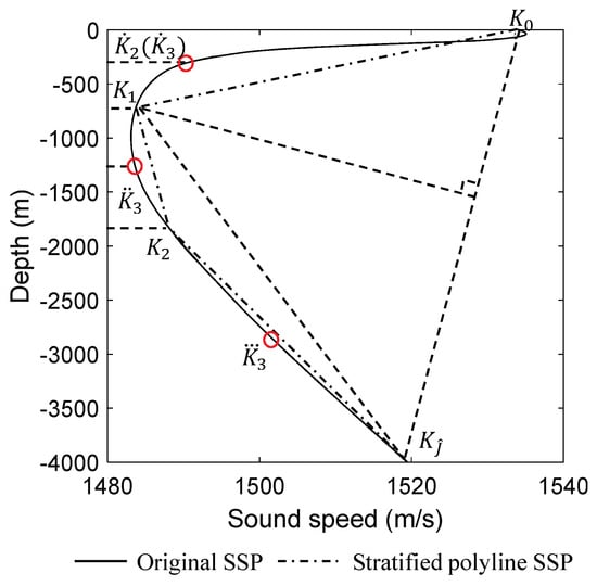
Figure 5.
Simplification of SVPs.
Optimization Searching of Signal Grazing Angle
In our localization scheme, there are several steps in each iteration that require initial signal grazing angle searching. If it can be proven that the signal propagation time and horizontal distance are convex functions, then mature optimization searching methods can be used, so as to significantly improve computational efficiency compared to traversal searching methods.
In this paper, we provide two properties and one corollary to prove that the signal propagation time and horizontal propagation distance are monotonic functions of the initial grazing angle. In accordance with Figure 6, let , where is the sound speed at depth , is the sound speed at depth , . Let be the grazing angle at depth , and be the grazing angle at depth ; there will be:
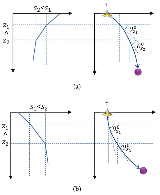
Figure 6.
Bending direction of signal propagation path. (a) SVP with negative gradient. (b) SVP with positive gradient.
Theorem 1.
For , if , that is , then ; if , that is , then [48].
Proof.
For a linear layered SVP with negative gradient as shown in Figure 6a, with and , according to Snell’s law of refraction, there is:
where is the grazing angle at depth . Since , then . For , there will be , which means the signal propagation path bends towards the direction where sound speed decreases (down). Similarly, for linear layered SVPs with a negative gradient as shown in Figure 6b, and . According to Equation (26), since , then . For , there will be , which means the signal propagation path bends towards the direction where sound speed decreases (up). To sum up, for a linear layered SVP, the signal propagation path bends in the direction where sound speed decreases. □
Referring to Figure 7, there will be:
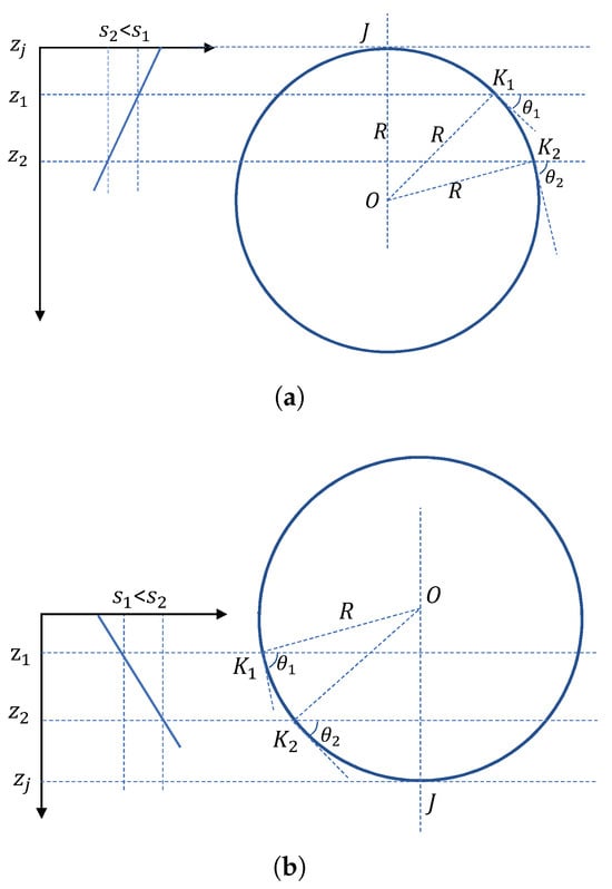
Figure 7.
Proof of arc trajectory. (a) SVP with negative gradient. (b) SVP with positive gradient.
Theorem 2.
For , if , and , where , there is [48].
Proof.
(by contradiction) It is shown in Figure 7a that , where is the gradient of sound speed. According to property 1, the signal propagation path will be down-curved. The signal is sent out from , and an auxiliary line in a direction perpendicular to the signal propagation direction at is set as . Let be a random point of the arc, and the angle between the tangent of the arc passing through points or and the horizontal direction are or .
Assume that is not a point on the signal propagation trajectory; there will be:
In fact, based on geometric relationships, there is:
Substitute ; there will be:
Since , there will be:
which means Equation (27) is not valid. Similarly, for any point at depth with , the same conclusion can be reached. Therefore, the signal propagation path is a segment of circle arc. Similar conclusions could be drawn in Figure 7b. In a word, for a linear layered SVP, the signal propagation path within any linear depth layer is an arc. □
Referring to Figure 8, there is:
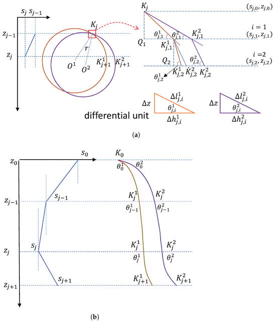
Figure 8.
Proof of monotonicity. (a) Micro-element perspective. (b) Macro perspective.
Theorem 3.
For , if , then and ; if , then and .
Proof of Corollary 1.
Assume that the gradient of an SVP is negative and the signal shoots from shallow water to deep water. Divide the signal trajectory with different initial grazing angles into I small segments for the ith depth layer as shown in Figure 8a. There is:
where . Since the gradient of sound speed is negative, there is . Let the depth be equally divided, and the space be . If is small enough, the propagation path of the signal in this depth space can be approximated by a straight line, so the propagation time of the signal is:
where . According to the equivalence relationship between definite integral and summation limit:
For the two paths shown in Figure 8a, if is proven, then there will be and .
When , let the grazing angles of two paths be and , respectively, which satisfies . Because , then will satisfy ; then:
For , according to Snell’s law:
Since , then and , which indicates that at the second depth layer there is still . When repeating the proof process for , there will be . Finally, we obtain and .
Similarly, it can be proven that for SVP layers with positive gradient, the propagation time and horizontal propagation distance of signals are also monotonically decreasing functions of the initial grazing angle. For SVPs with multiple linear layers as shown in Figure 8b, if , there will be and based on the above proof process. Finally, there is:
which proves corollary 1 that for a linear layered SVP, the propagation time and horizontal propagation distance of non-reflected signals are monotonically decreasing functions of the initial grazing angle. □
Based on the aforementioned analysis, the initial grazing angle can be searched through dichotomy, and the ray tracking process can be accelerated through SVP simplification, which helps achieve the fast operation of IRTUL.
3.3.2. Fast Algorithm of IRTUL
In this section, we give the fast algorithm of IRTUL as shown in Algorithm 1. To start with, based on the measured signal propagation time, the target localization is carried out using the average sound speed and linear propagation model. Then, the depth will be assumed as a known parameter, and horizontal repositioning will be performed based on the optimal matching of signal propagation time, and the matching cost function of signal propagation time before depth adjustment is calculated. Next, perform depth adjustment and calculate the cost function for matching the signal propagation time after depth adjustment. By comparing the two matching cost functions, whether the iteration process stops and how direction and step size of the next round of depth steps should be adjusted can be determined.
| Algorithm 1 Fast IRTUL Algorithm. |
|
4. Experiment Results
4.1. Parameter Settings
To verify the accuracy and efficiency performance of the proposed IRTUL algorithm, we conduct a simulation experiment in this section for testing. The simulation is conducted with Matlab (2023a). The simulation experiment parameters are shown in Table 1. The system error for measuring signal propagation time is set to 0.1% of the distance range, following zero-mean2 white Gaussian noise with standard deviation according to [9,22]. Thus, when the average sound speed is assumed to be 1500 m/s, the equivalent signal propagation time error will be s.

Table 1.
Parameter settings.
The simulation scenario is provided in Figure 9, where 25 surface buoys are uniformly distributed, and their positioning coordinates are obtained via GPS. Twenty-five anchors are also uniformly distributed at the bottom, and their location is known (obtained through positioning by buoys). Two-hundred nodes to be located are randomly suspended in water.
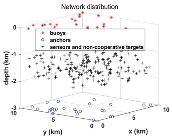
Figure 9.
Simulation scenario of network.
4.2. Simulation Results
4.2.1. Accuracy Performance
To verify the feasibility of using simplified SVPs in positioning systems, we provide localization accuracy results for different simplified methods of SVP as shown in Figure 10. The positioning RMSE errors of the total 200 sensors or non-cooperative targets are given in Figure 10a, where the curve of the proposed DM-EICPS is almost at the bottom, indicating that the simplified SVP via DM-EICPS for positioning has better accuracy performance. The average and standard deviation of localization errors by constant speed, original linear SVP and DM-EICPS simplified SVP are shown in Figure 10b. This shows that the positioning error of the simplified SVP is slightly greater than the result using the original SVP, but the difference is very small. If the number of layers in the simplified SVP is further increased, the positioning results will become closer to the positioning results by using the original SVP.
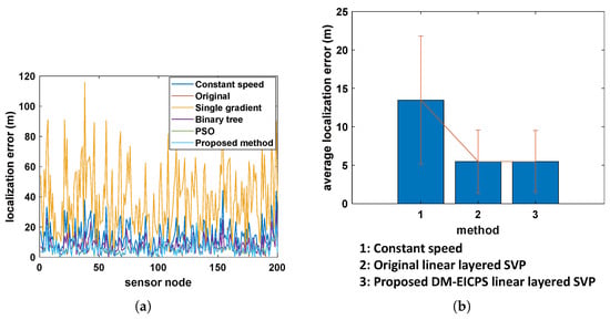
Figure 10.
Accuracy perpformance with different kinds of SVP simplification methods. (a) Two-hundred nodes. (b) Average results.
To further evaluate the accuracy performance of the proposed algorithm, we compare the localization errors under 50 times with those of JSL [22], which is given in Figure 11. The average localization error of ITRUL is 5.33 m, which has been reduced about 41% according to the average localization error 9.04 m of JSL.
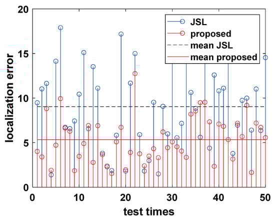
Figure 11.
Accuracy comparison of ITRUL with JSL.
Table 2 gives the average localization error of 200 nodes and increase of distance correction in the direction of x, y and z, respectively, when the threshold of depth tuning step is set to be 0.2 m. The results show that compared to the positioning model with constant sound speed, IRTUL has the most significant distance correction in the depth direction. Figure 12 gives a more intuitive correction result of pseudo range. The average accuracy of IRTUL has been improved by about 3 m.
Table 2.
Average positioning error and increase in distance correction.
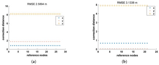
Figure 12.
Range correction performance of ITRUL. (a) Sensor node 1. (b) Sensor node 2.
In order to verify the convergence stability of the IRTUL method, Figure 13 shows the convergence of two sets of data. It can be seen that when the number of iterations exceeds 7 and 15, respectively, in Figure 13a,b with the initial depth tuning step set to be 1, the positioning process shows convergence, and the positioning accuracy is significantly improved compared to the constant speed situation. By increasing the initial depth tuning step to 2 or 3, the convergence will be accelerated according to Figure 13c–f; however, the initial depth tuning step could not be set too large as the convergence performance will not be stable and smooth as shown in Figure 13e,f.
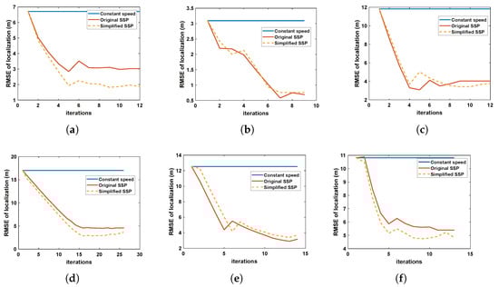
Figure 13.
Convergence performance of ITRUL. (a) Sensor node 1 with initial depth tuning step = 1. (b) Sensor node 1 with initial depth tuning step = 2. (c) Sensor node 1 with initial depth tuning step = 3. (d) Sensor node 2 with initial depth tuning step = 1. (e) Sensor node 2 with initial depth tuning step = 2. (f) Sensor node 2 with initial depth tuning step = 3.
4.2.2. Efficiency Performance
Although the positioning accuracy using a simplified SVP is slightly lower than that using the original SVP, the former can greatly reduce the computational complexity of ray tracing and the time cost of the positioning correction algorithm. To verify the time effectiveness of the positioning correction algorithm using a simplified SVP, Figure 14 compares the average time of positioning process using a simplified SVP with that using the original SVP under 10 test times. The results show that the time improvement effect is very significant with an average accuracy loss of less than 0.2 m when used for positioning.
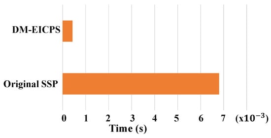
Figure 14.
Time efficiency of ITRUL.
4.2.3. Evaluation of ITRUL with Ocean Experiment
Besides simulation, we evaluate the practicality of the proposed ITRUL through data collected in the experiment at the South China Sea in April 2023. The scenario is shown in Figure 15. We sank the node to a depth of approximately 3500 m using heavy objects, and at the same time, we measured real-time SVP information using a sound velocity profiler. The mobile ship navigated around the deployment point in circular trajectories with a radius of 3 km. During the movement, it interacted with seabed nodes through the carried transducer and recorded the round-trip time information of the signal. The real-time position of the mobile ship was collected though the global positioning system.
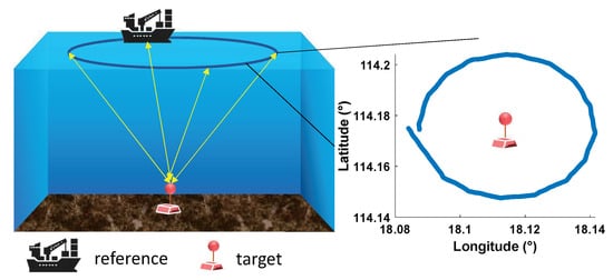
Figure 15.
Submarine node positioning test.
Due to the inability to obtain the accurate location of underwater targets during sea trials, we first evaluated the algorithm performance based on the principle of maximum likelihood estimation by comparing the deviation between simulated signal propagation time and sonar observation data. The average signal propagation time error and some of the testing results are given in Table 3. Furthermore, we compared the positioning error by sailing clockwise and counterclockwise, and the results in different directions are given in Table 4. The results show that the positioning algorithm achieved a meter level positioning error in sea trials.
Table 3.
Comparison of signal propagation time in sea trials by sailing clockwise.
Table 4.
Positioning deviation of clockwise and counterclockwise trajectory.
5. Conclusions
In this paper, we propose an IRTUL method for fast underwater target localization which addresses the issue of sound line bending and positioning accuracy degradation caused by uniformly distributed sound speed. Firstly, the monotonic relationship between signal propagation time and horizontal propagation distance with respect to the initial grazing angle is proved, so that binary search can be used to quickly obtain the initial grazing angle of the sound line. Then, we establish the IRTUL model. By using ray tracing and depth iterative tuning, the real signal propagation path of the signal can be effectively tracked in the case of unknown target depth, which improves the positioning accuracy. To reduce the computational complexity of the ray-theory-based sound correction process, an adaptive linear simplification method for SVPs based on minimizing the maximum distance criterion is proposed as DM-EICPS. Compared with the traditional simplification method for contour feature extraction, DM-EICPS exhibits higher positioning accuracy while significantly reducing the computational cost compared to the positioning with original SVPs.
Author Contributions
Conceptualization, W.H., K.M., T.X. and H.Z.; Data curation, W.S. and J.S.; Funding acquisition, W.H., T.X. and H.Z.; Methodology, W.H., K.M., T.X. and H.Z.; Project administration, T.X. and H.Z.; Software, W.S. and J.S.; Writing—review & editing, T.X. All authors have read and agreed to the published version of the manuscript.
Funding
This work was supported by Laoshan Laboratory (LSKJ202205104), Natural Science Foundation of Shandong Province (ZR2023QF128), China Postdoctoral Science Foundation (2022M722990 and 2022M723888), Qingdao Postdoctoral Science Foundation (QDBSH20220202061), National Natural Science Foundation of China (62271459), Central University Basic Research Fund of China, Ocean University of China (202313036).
Institutional Review Board Statement
Not applicable.
Informed Consent Statement
Not applicable.
Data Availability Statement
The data presented in this study are available on request from the corresponding author.
Conflicts of Interest
The authors declare no conflict of interest.
References
- Tan, H.P.; Diamant, R.; Seah, W.K.G.; Waldmeyer, M. A survey of techniques and challenges in underwater localization. Ocean Eng. 2011, 38, 1663–1676. [Google Scholar] [CrossRef]
- Qu, F.; Wang, S.; Wu, Z.; Liu, Z. A Survey of Ranging Algorithms and Localization Schemes in Underwater Acoustic Sensor Network. Chin. Commun. 2016, 13, 66–81. [Google Scholar]
- Junhai, L.; Liying, F.; Shan, W.; Xueting, Y. Research on Localization Algorithms Based on Acoustic Communication for Underwater Sensor Networks. Sensors 2018, 18, 67. [Google Scholar] [CrossRef] [PubMed]
- Luo, J.; Yang, Y.; Wang, Z.; Chen, Y. Localization Algorithm for Underwater Sensor Network: A Review. IEEE Internet Things J. 2021, 8, 13126–13144. [Google Scholar] [CrossRef]
- Jensen, F.B.; Kuperman, W.A.; Porter, M.B.; Schmidt, H. Computational Ocean Acoustics: Chapter 1; Springer Science & Business Media: Berlin/Heidelberg, Germany, 2011; pp. 3–4. [Google Scholar]
- Cheng, X.; Shu, H.; Liang, Q.; Du, D.H.C. Silent Positioning in Underwater Acoustic Sensor Networks. IEEE Trans. Veh. Technol. 2008, 57, 1756–1766. [Google Scholar] [CrossRef]
- Cheng, W.; Thaeler, A.; Cheng, X.; Liu, F.; Lu, X.; Lu, Z. Time-Synchronization Free Localization in Large Scale Underwater Acoustic Sensor Networks. In Proceedings of the 2009 29th IEEE International Conference on Distributed Computing Systems Workshops, Montreal, QC, Canada, 22–26 June 2009; pp. 80–87. [Google Scholar] [CrossRef]
- Liu, B.; Chen, H.; Zhong, Z.; Poor, H.V. Asymmetrical Round Trip Based Synchronization-Free Localization in Large-Scale Underwater Sensor Networks. IEEE Trans. Wirel. Commun. 2010, 9, 3532–3542. [Google Scholar] [CrossRef]
- Carroll, P.; Mahmood, K.; Zhou, S.; Zhou, H.; Xu, X.; Cui, J.H. On-Demand Asynchronous Localization for Underwater Sensor Networks. IEEE Trans. Signal Process. 2014, 62, 3337–3348. [Google Scholar] [CrossRef]
- Yan, J.; Zhang, X.; Luo, X.; Wang, Y.; Chen, C.; Guan, X. Asynchronous Localization With Mobility Prediction for Underwater Acoustic Sensor Networks. IEEE Trans. Veh. Technol. 2018, 67, 2543–2556. [Google Scholar] [CrossRef]
- Berger, C.R.; Wang, Z.; Huang, J.; Zhou, S. Application of compressive sensing to sparse channel estimation. IEEE Commun. Mag. 2010, 48, 164–174. [Google Scholar] [CrossRef]
- Gwun, B.C.; Han, J.W.; Kim, K.M.; Jung, J.W. MIMO underwater communication with sparse channel estimation. In Proceedings of the 2013 Fifth International Conference on Ubiquitous and Future Networks (ICUFN), Da Nang, Vietnam, 2–5 July 2013; pp. 32–36. [Google Scholar] [CrossRef]
- Tüchler, M.; Singer, A.C. Turbo Equalization: An Overview. IEEE Trans. Inf. Theory 2011, 57, 920–952. [Google Scholar] [CrossRef]
- Jung, J.; Kim, K. Optimizing of Iterative Turbo Equalizer for Underwater Sensor Communication. Int. J. Distrib. Sens. Netw. 2013, 2013, 129781. [Google Scholar] [CrossRef]
- Mahmutoglu, Y.; Turk, K.; Tugcu, E. Particle swarm optimization algorithm based decision feedback equalizer for underwater acoustic communication. In Proceedings of the 2016 39th International Conference on Telecommunications and Signal Processing (TSP), Vienna, Austria, 27–29 June 2016; pp. 153–156. [Google Scholar] [CrossRef]
- Liu, K.W. Detection of Underwater Sound Source Using Time Reversal Mirror. In Proceedings of the 2019 IEEE Underwater Technology (UT), Kaohsiung, Taiwan, 16–19 April 2019; pp. 1–5. [Google Scholar] [CrossRef]
- Teymorian, A.Y.; Cheng, W.; Ma, L.; Cheng, X.; Lu, X.; Lu, Z. 3D Underwater Sensor Network Localization. IEEE Trans. Mob. Comput. 2009, 8, 1610–1621. [Google Scholar] [CrossRef]
- Zhou, Z.; Cui, J.H.; Zhou, S. Efficient localization for large-scale underwater sensor networks. Ad Hoc Netw. 2010, 8, 267–279. [Google Scholar] [CrossRef]
- Zhang, S.; Zhang, Q.; Liu, M.; Fan, Z. A top-down positioning scheme for underwater wireless sensor networks. Sci. China Inf. Sci. 2014, 57, 1–10. [Google Scholar] [CrossRef]
- Huang, H.; Zheng, Y.R. AoA assisted localization for underwater Ad-Hoc sensor networks. In Proceedings of the OCEANS 2016 MTS/IEEE Monterey, Monterey, CA, USA, 19–23 September 2016; pp. 1–6. [Google Scholar] [CrossRef]
- Diamant, R.; Lampe, L. Underwater Localization with Time-Synchronization and Propagation Speed Uncertainties. IEEE Trans. Mob. Comput. 2013, 12, 1257–1269. [Google Scholar] [CrossRef]
- Liu, J.; Wang, Z.; Cui, J.H.; Zhou, S.; Yang, B. A Joint Time Synchronization and Localization Design for Mobile Underwater Sensor Networks. IEEE Trans. Mob. Comput. 2016, 15, 530–543. [Google Scholar] [CrossRef]
- Zhang, L.; Zhang, T.; Shin, H.S.; Xu, X. Efficient Underwater Acoustical Localization Method Based On Time Difference and Bearing Measurements. IEEE Trans. Instrum. Meas. 2021, 70, 8501316. [Google Scholar] [CrossRef]
- Youngberg, J.W. A Novel Method for Extending GPS to Underwater Applications. Navigation 1991, 38, 263–271. [Google Scholar] [CrossRef]
- Erol-Kantarci, M.; Mouftah, H.T.; Oktug, S. A survey of architectures and localization techniques for underwater acoustic sensor networks. IEEE Commun. Surv. Tutor. 2011, 13, 487–502. [Google Scholar] [CrossRef]
- Niculescu, D.; Nath, B. Ad hoc positioning system (APS). In Proceedings of the GLOBECOM’01. IEEE Global Telecommunications Conference (Cat. No.01CH37270), San Antonio, TX, USA, 25–29 November 2001; Volume 5, pp. 2926–2931. [Google Scholar] [CrossRef]
- Niculescu, D.; Nath, B. DV based positioning in ad hoc networks. Telecommun. Syst. Model. Anal. Des. Manag. 2003, 22, 267–280. [Google Scholar] [CrossRef]
- He, T.; Huang, C.; Blum, B.M.; Stankovic, J.A.; Abdelzaher, T.F. Range-free localization schemes for large scale sensor networks. In Proceedings of the Ninth Annual International Conference on Mobile Computing and Networking, MOBICOM 2003, San Diego, CA, USA, 14–19 September 2003; pp. 81–95. [Google Scholar]
- Wong, S.Y.; Lim, J.G.; Rao, S.; Seah, W. Multihop localization with density and path length awareness in non-uniform wireless sensor networks. In Proceedings of the 2005 IEEE 61st Vehicular Technology Conference, Stockholm, Sweden, 30 May–1 June 2005; Volume 4, pp. 2551–2555. [Google Scholar] [CrossRef]
- Chandrasekhar, V.; Seah, W. An Area Localization Scheme for Underwater Sensor Networks. In Proceedings of the OCEANS 2006-Asia Pacific, Singapore, 16–19 May 2006; pp. 1–8. [Google Scholar] [CrossRef]
- Lee, S.; Kim, K. Localization with a Mobile Beacon in Underwater Acoustic Sensor Networks. Sensors 2012, 12, 5486–5501. [Google Scholar] [CrossRef] [PubMed]
- Zandi, R.; Kamarei, M.; Amiri, H.; Yaghoubi, F. Underwater Sensor Network Positioning Using an AUV Moving on a Random Waypoint Path. IETE J. Res. 2015, 61, 693–698. [Google Scholar] [CrossRef]
- Zhu, S.; Jin, N.; Wang, L.; Yang, S.; Zheng, X.; Zhu, M.; Sun, L. Error tolerant dual-hydrophone localization in underwater sensor networks. In Proceedings of the OCEANS 2016, Shanghai, China, 19–23 September 2016; pp. 1–4. [Google Scholar] [CrossRef]
- Erol, M.; Vieira, L.F.M.; Gerla, M. Localization with Dive’N’Rise (DNR) Beacons for Underwater Acoustic Sensor Networks. In Proceedings of the 2nd Workshop on Underwater Networks, New York, NY, USA, 14 September 2007; WUWNet ’07. pp. 97–100. [Google Scholar] [CrossRef]
- Isik, M.T.; Akan, O.B. A three dimensional localization algorithm for underwater acoustic sensor networks. IEEE Trans. Wirel. Commun. 2009, 8, 4457–4463. [Google Scholar] [CrossRef]
- Kurniawan, A.; Ferng, H.W. Projection-based localization for underwater sensor networks with consideration of layers. In Proceedings of the IEEE 2013 Tencon-Spring, Sydney, NSW, Australia, 17–19 April 2013; pp. 425–429. [Google Scholar] [CrossRef]
- Uddin, M.Y.S. Low-overhead range-based 3D localization technique for underwater sensor networks. In Proceedings of the 2016 IEEE International Conference on Communications (ICC), Kuala Lumpur, Malaysia, 23–27 May 2016; pp. 1–6. [Google Scholar] [CrossRef]
- Alexandri, T.; Walter, M.; Diamant, R. A Time Difference of Arrival Based Target Motion Analysis for Localization of Underwater Vehicles. IEEE Trans. Veh. Technol. 2022, 71, 326–338. [Google Scholar] [CrossRef]
- Weiss, A.; Arikan, T.; Vishnu, H.; Deane, G.B.; Singer, A.C.; Wornell, G.W. A Semi-Blind Method for Localization of Underwater Acoustic Sources. IEEE Trans. Signal Process. 2022, 70, 3090–3106. [Google Scholar] [CrossRef]
- Sun, S.; Zhao, C.; Zheng, C.; Zhao, C.; Wang, Y. High-Precision Underwater Acoustical Localization of the Black Box Based on an Improved TDOA Algorithm. IEEE Geosci. Remote Sens. Lett. 2020, 18, 1317–1321. [Google Scholar] [CrossRef]
- Sun, S.; Liu, T.; Wang, Y.; Zhang, G.; Liu, K.; Wang, Y. High-Rate Underwater Acoustic Localization Based on the Decision Tree. IEEE Trans. Geosci. Remote Sens. 2022, 60, 4204912. [Google Scholar] [CrossRef]
- Li, X.; Wang, Y.; Qi, B.; Hao, Y. Long Baseline Acoustic Localization Based on Track-Before-Detect in Complex Underwater Environments. IEEE Trans. Geosci. Remote Sens. 2023, 61, 4205214. [Google Scholar] [CrossRef]
- Ramezani, H.; Jamali-Rad, H.; Leus, G. Target Localization and Tracking for an Isogradient Sound Speed Profile. IEEE Trans. Signal Process. 2013, 61, 1434–1446. [Google Scholar] [CrossRef]
- Zhang, B.; Wang, H.; Zheng, L.; Wu, J.; Zhuang, Z. Joint Synchronization and Localization for Underwater Sensor Networks Considering Stratification Effect. IEEE Access 2017, 5, 26932–26943. [Google Scholar] [CrossRef]
- Zhang, Y.; Li, Y.; Zhang, Y.; Jiang, T. Underwater Anchor-AUV Localization Geometries With an Isogradient Sound Speed Profile: A CRLB-Based Optimality Analysis. IEEE Trans. Wirel. Commun. 2018, 17, 8228–8238. [Google Scholar] [CrossRef]
- Gong, Z.; Li, C.; Jiang, F. A Machine Learning-Based Approach for Auto-Detection and Localization of Targets in Underwater Acoustic Array Networks. IEEE Trans. Veh. Technol. 2020, 69, 15857–15866. [Google Scholar] [CrossRef]
- Yan, J.; Yi, M.; Yang, X.; Luo, X.; Guan, X. Broad-Learning-Based Localization for Underwater Sensor Networks with Stratification Compensation. IEEE Internet Things J. 2023, 10, 13123–13137. [Google Scholar] [CrossRef]
- Wang, D.; Shang, E. Underwater Acoustics (Second Edition): Chapter 3; China Science Publishing and Media Ltd.: Beijing, China, 2013; pp. 105–106. [Google Scholar]
- Huang, W.; Liu, M.; Li, D.; Cen, Y.; Wang, S. A Stratified Linear Sound Speed Profile Simplification Method for Localization Correction. In Proceedings of the 14th International Conference on Underwater Networks & Systems, Atlanta, GA, USA, 23–25 October 2019. WUWNet ’19. [Google Scholar] [CrossRef]
Disclaimer/Publisher’s Note: The statements, opinions and data contained in all publications are solely those of the individual author(s) and contributor(s) and not of MDPI and/or the editor(s). MDPI and/or the editor(s) disclaim responsibility for any injury to people or property resulting from any ideas, methods, instructions or products referred to in the content. |
© 2024 by the authors. Licensee MDPI, Basel, Switzerland. This article is an open access article distributed under the terms and conditions of the Creative Commons Attribution (CC BY) license (https://creativecommons.org/licenses/by/4.0/).