Short-Term Exhaust Gas Temperature Trend Prediction of a Marine Diesel Engine Based on an Improved Slime Mold Algorithm-Optimized Bidirectional Long Short-Term Memory—Temporal Pattern Attention Ensemble Model

Abstract

As the core component of a ship’s engine room, the operation of a marine diesel engine (MDE) directly affects the economy and safety of the entire vessel. Predicting the future changes in the status parameters of a MDE helps to understand the operational status, enabling timely warnings to the engine crew, and to ensure the safe navigation of the vessel. Therefore, this paper combines the temporal pattern attention mechanism with the bidirectional long short-term memory (BiLSTM) network to propose a novel trend prediction method for short-term exhaust gas temperature (EGT) forecasting. First, the Pearson correlation analysis (PCA) is conducted to identify input feature variables that are strongly correlated with the EGT. Next, the BiLSTM network models input feature variables such as load, fuel oil pressure, and scavenging air pressure and capture the interrelationships between different vectors from the hidden layer matrix within the BiLSTM network. This allows the selection of valuable information across different time steps. Meanwhile, the temporal pattern attention (TPA) mechanism has the ability to explore complex nonlinear dependencies between different time steps and series. This assigns appropriate weights to the feature variables within different time steps of the BiLSTM hidden layer, thereby influencing the input effect. Finally, the improved slime mold algorithm (ISMA) is utilized to optimize the hyperparameters of the prediction model to achieve the best level of short-term EGT trend prediction performance based on the ISMA-BiLSTM-TPA model. The prediction results show that the mean square error, the mean absolute percentage error, the root mean square error and the coefficient of determination of the model are 0.4284, 0.1076, 0.6545 and 98.2%, respectively. These values are significantly better than those of other prediction methods, thus fully validating the stability and accuracy of the model proposed in this paper.

1. Introduction

Since the beginning of the 21st century, the volume of global trade has been continuously increasing, driving the rapid development of the shipping industry, especially in the field of ocean shipping [1]. This trend has also spurred the maritime industry to move towards intelligence, with enhancing the automation and intelligence levels of ships becoming a focal point [2,3]. As the core power unit in a ship’s engine room, MDEs not only provide propulsion for ship navigation, but also drive generators to provide continuous and stable power for the entire ship’s operation [4]. The internal structure of MDEs is complex and relies on the coordinated operation of multiple subsystems. Any malfunction can adversely affect their operating performance, resulting in poor working conditions and reducing overall efficiency. In severe cases, engine shutdowns can occur, damaging associated equipment, disrupting the normal operation of the vessel, and posing a risk to the safety of personnel and property on board [5]. Due to prolonged exposure to harsh operating environments, MDE components experience severe wear, significantly increasing the risk of potential malfunctions and failures [6], However, traditional MDE condition monitoring techniques typically focus on monitoring the thermodynamic parameters of the engine, such as gas pressure and oil temperature. These parameters only show significant changes when the malfunction has reached a certain severity [7]. Therefore, traditional condition monitoring techniques cannot predict the future trend of diesel engine status changes over a period of time. In contrast, more mature condition monitoring techniques utilize intelligent algorithms to learn from historical diesel engine operating data. Using the powerful nonlinear computing capabilities of intelligent algorithms, these techniques can calculate the trend changes in diesel engine status parameters over a period of time. By observing the trend changes in the status parameters, early warnings can be issued to effectively prevent potential failures. Therefore, by studying the condition monitoring technology of MDE to predict the trend changes in their status parameters, faults can be detected in a timely manner during the latent period and relevant warnings can be issued. This not only gives the engine crew enough time to inspect the related equipment, but also reduces the subsequent maintenance costs and ensures the efficient operation of MDE. This is of paramount importance in improving the reliability of MDE.

The EGT is an important thermal parameter of MDE. To a certain extent, it can characterize the operating condition of the MDE and the load distribution of each cylinder [8]. Different degrees of variation in the EGT can reflect faults in different subsystems of the MDE, and the temperature changes relatively slowly with minimal interference from external factors [9]. Real-time monitoring and prediction of the EGT can provide insight into the health status of MDE, ensuring the normal operation of ships [10].

Currently, trend prediction research methods mainly focus on physics-based modeling and data-driven approaches. Model-based methods require the construction of accurate physical or mathematical models to describe the operational processes of the research object [11]. Model-based methods face significant challenges in constructing accurate models of marine equipment in complex and dynamic environments such as ship engine rooms. In contrast, data-driven methods avoid the cumbersome modeling process. This method uses historical data collected by monitoring systems as the research object [12], and conducts data analysis and processing, and uses relevant intelligent algorithms to establish trend prediction models, eliminating the influence of complex environmental changes on the trend of ship equipment status parameters. By establishing a unified standard trend prediction curve, engineers can assess the status of MDEs in advance by observing the trend changes in the EGT over a period of time, achieving real-time online monitoring of ships. In recent years, with the continuous updating and iteration of Internet technology, related intelligent algorithms have emerged. The data-driven equipment status parameter trend prediction has attracted widespread attention from industry professionals [13].

Liu et al. analyzed the vibration signals of diesel engines, extracted fitted characteristic parameters, and successfully established a prediction model for the performance trend of diesel engines using radial basis function (RBF) neural networks, thereby improving the prediction accuracy [14]. Cui et al. 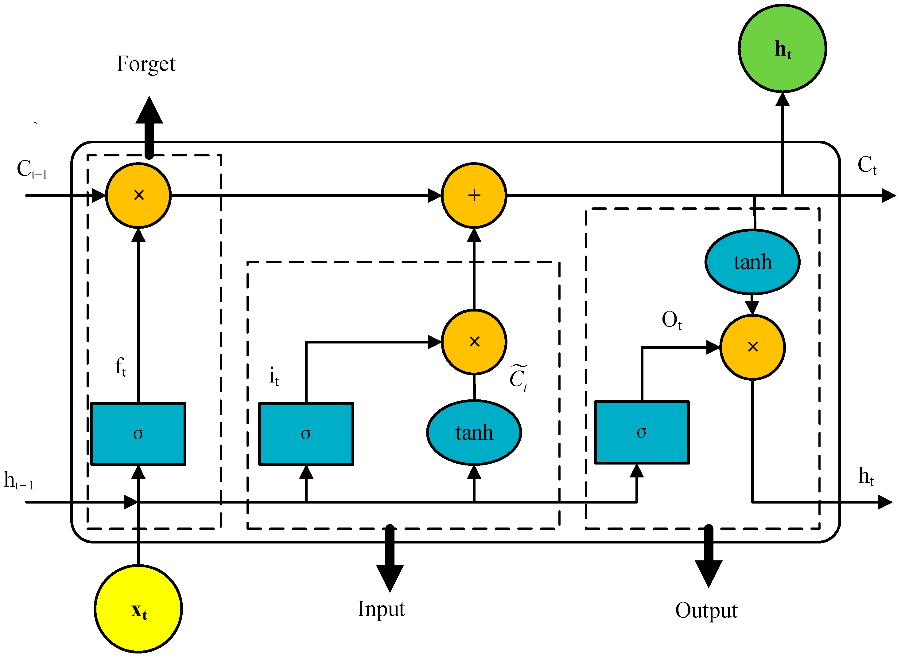developed a degradation model for solid oxide fuel cells (SOFCs) based on the area-specific resistance (ASR) and successfully predicted the full-cycle degradation trend of SOFCs using the particle filtering algorithm [15]. Wang et al. utilized the comprehensive degradation index (CDI) in the time-frequency domain and long short-term memory (LSTM) to construct a trend prediction model for the state of hydropower units, achieving the prediction of the degradation trend of hydropower units and improving the prediction accuracy [16]. Theerthagiri et al. utilized the Seasonal ARIMA (SARIMA) model combined with the weighted average method and feedback error analysis method to forecast crude oil prices, successfully improving the prediction accuracy and obtaining a more accurate trend of crude oil price changes [17]. Xu et al. developed a greenhouse microclimate trend prediction model based on an improved empirical mode decomposition (IEMD)-optimized informer. By utilizing data from five different environmental factors, the model accurately predicts the development trend of environmental factors [18]. Zhao et al. utilized an improved AO algorithm to optimize the support vector regression (SVR) prediction model, and achieved the matching of corresponding optimal parameters under different operating conditions. This allowed for the accurate prediction of the development trend of various operating state indicators of hydropower units over a certain time scale [19]. Li et al. used the LSTM method to establish a trend prediction model for the wear state parameters of oil products. They used the prediction results as the test set to establish a deep belief networks (DBN) prediction model for predicting device power. This method achieved continuous prediction of the wear state of lubricating oil with objective factors and was successfully applied to the prediction of power trends of power plant turbines with subjective factors [20]. Zhang et al. employed an LSTM network to establish a multi-input multi-output model for predicting the EGT of MDE. They validated the effectiveness of this model using historical operational data from actual ships [8]. Liu et al. utilized an attention mechanism and a LSTM network to establish a trend prediction model for the EGT of MDE. They optimized the LSTM network parameters using the particle swarm algorithm, thereby improving the accuracy of the prediction model. Additionally, they implemented fault prediction by analyzing the distribution of residuals between predicted and actual values [21]. Li et al. used the chaotic bat algorithm to optimize the hyperparameters of the LightGBM network and established a trend prediction model for the EGT of aircraft engines. They demonstrated the model’s effectiveness in monitoring the performance of aircraft engines using historical operational data from a specific aircraft engine [22].

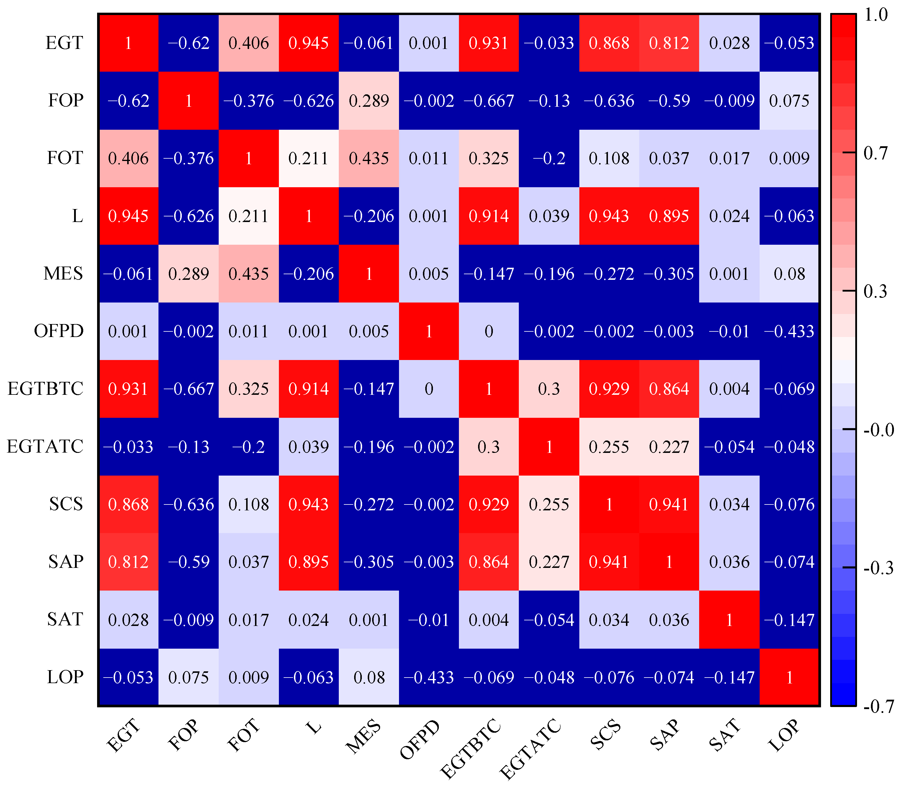
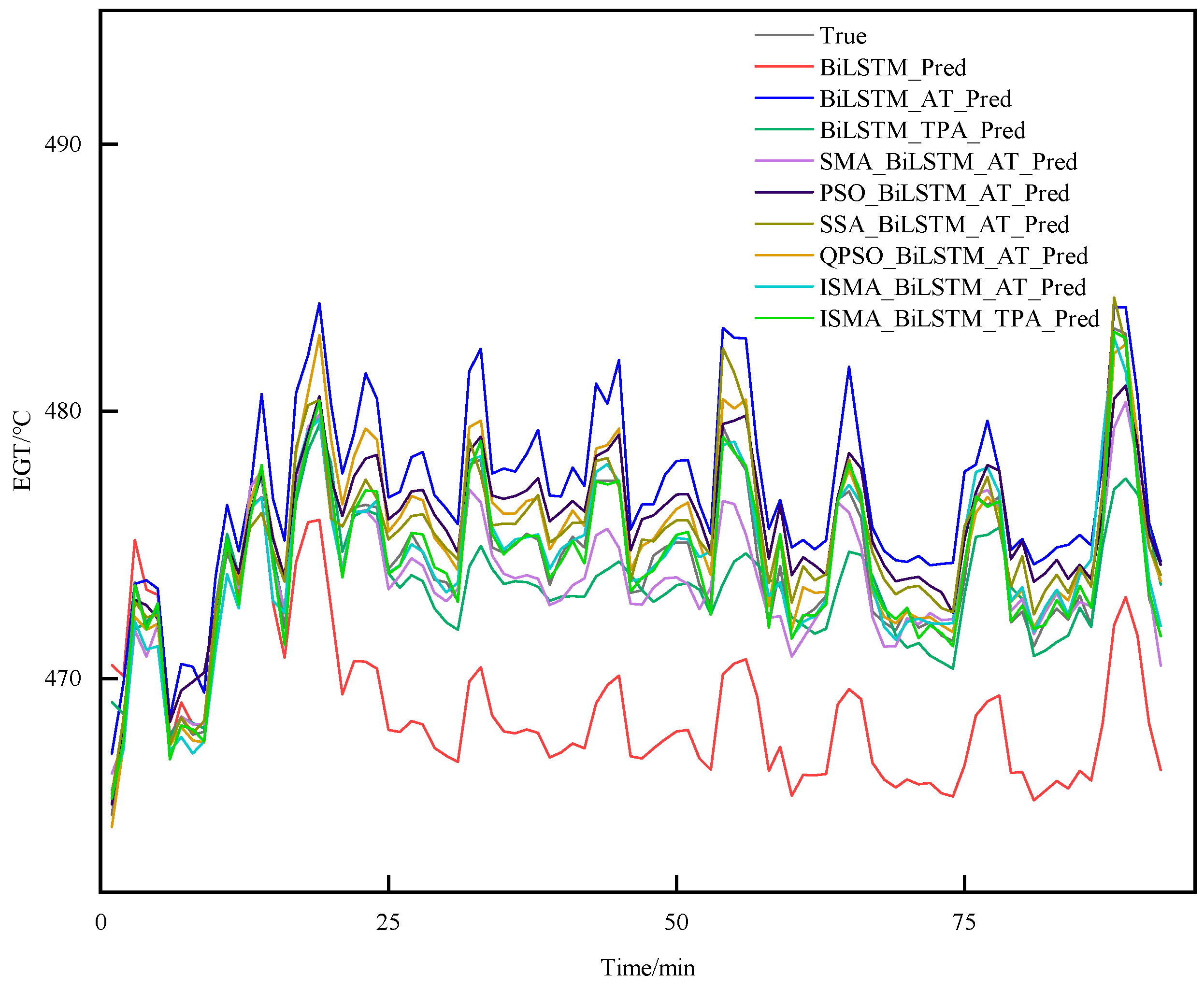
The existing trend prediction research can be divided into two main categories: equipment degradation trend prediction models and real-time equipment status trend prediction models. Equipment degradation trend prediction methods require the use of operational data from the entire lifecycle of the equipment as the research object MDEs. Currently, there is limited research on real-time status monitoring of MDEs, despite their critical role in ensuring the safe navigation of ships and the safety of crew and property. Therefore, this paper proposes a trend prediction method based on a BiLSTM-TPA neural network for short-term EGT trend prediction. Firstly, the PCA method is used to determine the feature variables with strong correlation to the EGT as the inputs to the model, thereby avoiding redundant input feature vectors. Then, the BiLSTM network is employed to learn the internal positive and negative features among the input variables. The TPA mechanism is integrated to further capture the inherent relationships among the variables under different sequences and time steps. Finally, the ISMA is used to optimize the hyperparameters of the BiLSTM-TPA network to obtain the EGT trend. This paper critically reviews the challenges in predicting the status parameters of MDE-related equipment, highlighting issues such as insufficient prediction accuracy and inappropriate selection of parameters. In response, it introduces a novel short-term trend prediction method for the EGT of MDEs, designated as the ISMA-BiLSTM-TPA. This method effectively addresses the latency issues inherent in traditional time-series prediction models. Comparative analyses with existing algorithms demonstrate the superior performance of the proposed method, evidenced by significant improvements across several metrics. Specifically, the MSE values decreased by 36.9302, 8.0956, 2.9568, 0.7334, 1.1768, and 0.4284; the MAPE values were reduced by 1.0823%, 0.4639%, 0.1679%, 0.084%, 0.1133%, and 0.0158%; the RMSE values saw reductions of 5.6775, 2.2645, 1.1848, 0.4234, 0.6130, and 0.1506; and the R2 values experienced increments of 16.9%, 11.8%, 9.70%, 7.4%, 5.7%, and 2.4%, respectively. These results not only underscore the efficacy of the ISMA-BiLSTM-TPA approach in enhancing predictive accuracy but also its potential in revolutionizing the domain of MDE monitoring and predictive analysis.

The subsequent sections of this paper cover the following content: Section 2 introduces methods such as Pearson correlation analysis (PCA), BiLSTM model, TPA mechanism, and the SMA based on reverse learning and hybrid nonlinear inertia weight decay. Section 3 discusses the short-term trend prediction of the EGT of MDE based on the ISMA-BiLSTM-TPA model, including the evaluation index of the prediction model and experimental setup configurations. Section 4 introduces the research object and experimental data, organizes input feature parameters and experimental data, and sets optimization parameters for the prediction model. Finally, the analysis and discussion of the short-term EGT trend prediction results for the 6L34DF type are presented, followed by conclusions in the concluding section.

2. Method

2.1. The PCA Method

PCA is a statistical tool primarily utilized to assess the degree of linear correlation between two variables. The purpose is to uncover the interrelationships between variables. This method finds extensive application in scenarios involving data analysis and data dimensionality reduction [23,24]. In the process of correlation analysis, the PCC serves as a crucial measure for assessing the correlation between two variables. Assuming the sample size for the relevant parameters of the EGT is denoted by m, after dimensionless transformation of the original dataset, the correlation coefficient is calculated as follows in Equation (1):

$$r_{xy}=\frac{{\displaystyle \sum _{i=1}^m\left(x_i-\stackrel{-}{x}\right)\left(y_i-\stackrel{-}{y}\right)}}{\sqrt{{\displaystyle \sum _{i=1}^m\left(x_i-\stackrel{-}{x}\right)}}\sqrt{{\displaystyle \sum _{i=1}^m\left(y-\stackrel{-}{y}\right)}}}$$

(1)

In the equation, $r_{xy}$ is a statistical measure quantifying the degree of linear correlation between $x$ and $y$, which used to describe the extent of their association. $r\in \left[-1,1\right]$; $x=\left[x_1,x_2,\cdots ,x_m\right],y=\left[y_1,y_2,\cdots ,y_m\right]$; x represents the input variable related to the EGT, and $y$ represents the EGT; $\stackrel{-}{x}$ and $\stackrel{-}{y}$ represent the mean values of $x_i$ and $y_i$, respectively. When $r_{xy}>0$, which indicates a positive correlation between $x$ and $y$. When $r_{xy}<0$, which indicates a negative correlation between $x$ and $y$. When $r_{xy}=0$, $x$ and $y$ are uncorrelated. If the absolute value of the correlation coefficient is close to 0, it indicates a weak association between the variable [25]. Under normal circumstances, the correlation strength of variables can be evaluated based on the values in

Table 1. The evaluation criteria for the Pearson correlation coefficient.

The Range of Values for $\left|\mathit{r}\right|$	The Degree of Correlation
$0\le \left|r\right|<0.1$	Uncorrelated
$0.1\le \left|r\right|<0.4$	Weak correlation
$0.4\le \left|r\right|<0.6$	Moderate correlation
$0.6\le \left|r\right|<0.8$	Strong correlation
$0.8\le \left|r\right|\le 1.0$	Very strong correlation

.

2.2. The BiLSTM Model

The BiLSTM network is derived from the LSTM network and is mainly composed of two LSTM layers, one in the forward direction and one in the backward direction. LSTM is an improvement over the recurrent neural network (RNN), effectively addressing the challenges of long-term dependencies and gradient vanishing faced by traditional RNNs by introducing specific mechanisms [26]. As one of the recursive neural networks, LSTM utilizes gate units to regulate the transmission state of information, preserving crucial long-term memory while suppressing the influence of minor information. The structure is illustrated in Figure 1.

From Figure 1, it can be observed that LSTM is primarily composed of three special “gate” structures that selectively control the state of the network at each time step, wherein $C_{t-1}$ denotes the effective state stored in the cell at the previous time step; $h_{t-1}$ denotes the output of information from the previous time step; $x_t$ denotes the input information at the current time step; $f_t$ denotes the forget gate, which determines the degree of forgetting of information; $i_t$ denotes the input gate, determining which content participates in the update of $C_t$. $\widetilde{C_t}$ denotes the current cell state; $O_t$ determines the output information at the current time step; tanh denotes the activation function of the network, typically using the hyperbolic tangent function when updating cell unit states; $\sigma$ denotes the sigmoid activation function used in gate units.

$$f_t=\sigma \left(W_f\left[h_{t-1},x_t\right]+b_f\right)$$

(2)

$$i_t=\sigma \left(W_i\left[h_{t-1},x_t\right]+b_i\right)$$

(3)

$$\widetilde{C_t}=\tanh \left(W_c\left[h_{t-1},x_t\right]+b_c\right)$$

(4)

$$C_t=\sigma \left(f_t·C_{t-1}+i_t\otimes \widetilde{C_t}\right)$$

(5)

$$O_t=\sigma \left(W_o\left[h_{t-1},x_t\right]+b_o\right)$$

(6)

$$h_t=O_t·\tanh \left(C_t\right)$$

(7)

In the equation, $W_f$, $W_i$, $W_c$ and $W_o$—weight threshold; $b_f$, $b_i$, $b_c$ and $b_o$—bias parameters.

The BiLSTM network processes temporal sequences bidirectionally, integrating bidirectional information into a single output to comprehensively understand the interdependencies in the time series. This aids in mitigating the issue of early information loss caused by long sequences, and makes it applicable for predicting short-term trends in the EGT of MDE. Refer to Figure 2 for the specific architecture.

2.3. The Temporal Pattern Attention Mechanism

The attention mechanism (AT) plays a significant role in mimicking human attention. It allows the model to focus on processing information relevant to specific tasks, similar to how the human brain processes information. This mechanism demonstrates versatile application potential in various areas such as language processing, image analysis, and prediction tasks [27,28,29]. It enables models to deeply utilize crucial information from historical data, thereby enhancing the ability to recognize and utilize key patterns. Additionally, it possesses the capability to review information from previous time steps and focus on task-relevant information, thereby coordinating to generate more accurate output results. However, classical attention mechanisms primarily focus on weighting individual variables within each time step, which may not effectively calculate variable weights for complex nonlinear variables like the EGT of MDE, which are influenced by multiple factors within a single time step, thereby affecting model performance to some extent. In 2019, Shih and their team proposed a novel approach called the TPA mechanism based on improving self-attention mechanisms [30]. The TPA mechanism can capture the interrelations between multiple variables within the current time step and their cross-correlations with all previous time series. It employs a scoring function to weight the calculation of each indicator, which to some extent improves the model’s performance. The ultimate output is derived by aggregating the calculation results of each indicator. The working principle is illustrated in Figure 3.

In this paper, the TPA mechanism is integrated with the BiLSTM network. During the operation of the combined model, the TPA mechanism utilizes an internal one-dimensional convolutional neural network (CNN) filter to extract key information from the hidden state row vector matrix of the BiLSTM network. For processing data related to the EGT of MDE, the operational procedure of TPA mainly includes the following steps.

Step 1: Set $h=\left\{h_{m,\left(t-\omega +1\right)},\cdots ,h_{m,t}\right\}$ as the input sequence of EGT data related to MDE for TPA, where ω denotes the size of the data sequence, and $m$ denotes the dimensionality of the data sequence. $C=\left\{C_1,C_2,\dots ,C_T\right\}$ denotes the CNN filter, $T$ denotes the maximum length of TPA, and let $\omega =T$. It is necessary to maintain the sequence length the same as the length obtained by TPA. After convolving $h$ and $C$ with the filter, the corresponding temporal patterns are obtained as follows:

$$H_{i,j}^C={\displaystyle {\sum }_{l=1}^{\omega }{h}_{i,\left(t-\omega -1+l\right)}\times C_{j,T-\omega +l}}$$

(8)

Step 2: Select the sigmoid function as the activation function and define f as the evaluation function. After calculating the weights, the result is obtained as:

$$f\left(H_i^C,h_{m,t}\right)={\left(H_i^C\right)}^T{W}_a{h}_t$$

(9)

$${\alpha }_i=sigmoid\left(f\left(H_i^C,h_t\right)\right)$$

(10)

In the equation, $H_i^C$ denotes the ith row vector of $H^C$, $W_a\in R^{m\times k}$ denotes the corresponding weight parameter, ${\alpha }_i$ denotes the weight parameter of $H_i^C$, i = 1, 2, …, m. After weighting ${\alpha }_i$ and $H^C$, and summing them, the attention expression is obtained as:

$$v_t={\displaystyle \sum _{i=1}^m{\alpha }_i{H}_i^C}$$

(11)

where m denotes the dimensionality of the input feature variables.

The summation of $h_t$ and $v_t$ after linear mapping yields the predicted value $y_{t-1+△}$ of the BiLSTM-TPA model.

$$y_{t-1+\Delta }=W_{h^{\prime }}\left(W_h{h}_t+W_v{v}_t\right)$$

(12)

Here, $W_{h^{\prime }}$, $W_h$ and $W_V$ denote the matrix parameter for calculating weights.

2.4. Based on the Backward Learning Mixed Nonlinear Inertial Weight Decay SMA Optimization Algorithm

In this section, we introduce the reverse learning and the nonlinear inertia weight decay strategy, which are based on the traditional slime mold algorithm (SMA) optimization. These strategies aim to strike a balance between the algorithm’s global search and local development capabilities, thus preventing premature convergence to local optima and facilitating the rapid discovery of the global optimal position. By applying this optimization algorithm, the prediction accuracy of the BiLSTM-TPA model is significantly enhanced after hyperparameter optimization.

2.4.1. The SMA Optimization Algorithm

The SMA is an optimization algorithm derived from observing the behavior of slime molds as they move and form grid-like structures when searching for food and responding to environmental stimuli [31]. The algorithm draws inspiration from the adaptive movement strategy of slime mold populations in environments with uneven food distribution to find the optimal foraging path and solve various optimization problems [32,33,34]. the optimization process mainly includes the following three stages:

Stage 1: Approaching Food. Slime mold populations rely on sensing the odor released by food in the air to search for the location of food. The specific method is detailed in Equation (12).

$$Y\left(t+1\right)=\left\{\begin{array}{l}{Y}_b\left(t\right)+v_b·\left(W·Y_{rand1}\left(t\right)-Y_{rand2}\left(t\right)\right),r>p\\ v_c·Y\left(t\right),r<p\end{array}\right.$$

(13)

In the t-th iteration process, Y(t) denotes the position of the slime mold; Y_b(t) indicates the position of the slime mold at the current individual with the best fitness. The iteration count of the slime mold is denoted by t; r denotes any arbitrary number between 0 and 1. The value of v_b is within the range of [−a, a]; v_c denotes a linearly decreasing number between 1 and 0; Y_rand1(t) and Y_rand2(t) refer to the random positions of two slime mold individuals.

The equation for updating the maximum limits p and v_b, as well as the weight parameters and $a$, are as follows:

$$p=\tanh \left|S\left(i\right)-DF\right|,i\in 1,2,···,N$$

(14)

$$a=\mathrm{arctanh}\left(1-\frac{t}{t_{\max }}\right)$$

(15)

$$W\left(SmellIndex\left(i\right)\right)=\left\{\begin{array}{l}1+r·\log \left(\left(b_F-w_F\right)+1\right),condition\\ 1-r·\log \left(\left(b_F-w_F\right)+1\right),others\end{array}\right.$$

(16)

$$SmellIndex=sort\left(S\right)$$

(17)

where DF denotes the current population’s best fitness value; S(i) denotes the fitness value of an individual slime mold; N denotes the total number of slime molds in the population; condition represents the top 1/2 ranking individuals in the slime mold population based on their S(i) values. The remaining individuals in the population are denoted by others; t_max denotes the maximum number of iterations; b_F denotes the best fitness value attained by an individual during the current iteration process; W_F denotes the best fitness value attained by an individual during the current iteration process; Sort means to arrange the population’s fitness values in ascending order; SmellIndex denotes the sequence after arranging fitness values in order.

Stage 2: Food Encirclement. By simulating the positive and negative feedback regulation of their own position based on the concentration of food within the vein-like structures inside the slime mold body, they gradually encircle the food. The position updating strategy is as follows:

$$Y\left(t+1\right)=\left\{\begin{array}{l}rand\left(u_b-l_b\right)+l_b,r<z\\ Y_b\left(t\right)+v_b\left(W·Y_{rand1}\left(t\right)-Y_{rand2}\left(t\right)\right),r<p\\ v_{c}Y\left(t\right),r\ge p\end{array}\right.$$

(18)

where u_b and l_b, respectively, denote the upper and lower boundary values of the search area; rand is a random number between 0 and 1 that allows the slime mold to disperse in any direction; z denotes the switching probability, determining whether the slime mold population is approaching the search for the optimal individual or continuing to search for other food sources.

Stage 3: Oscillation Phase. By adjusting the values of W, v_b, and v_c, the process of the slime mold population gradually approaching the food source is simulated. During the approach to the food source, the oscillation frequency of the slime mold population will increase as the concentration of food rises. v_b will oscillate repeatedly within [−a, a] and gradually approach 0 with an increase in the number of iterations, while v_c will oscillate repeatedly within [−1, 1] and ultimately approach 0.

2.4.2. The Reverse Learning Strategy

The reverse learning strategy [35] compensates for the limitation of the population’s exploration range during the random initialization stage by increasing the diversity of the population, thereby improving the quality of the optimal point. The central idea of this strategy is to evaluate the current population’s solution by generating a reverse solution during the optimization phase of the slime mold population. By comparing the function values of the two, the more optimal solution is selectively retained as the starting point for the next round of iterative calculations. Suppose there exists a point $Y=\left[Y_1,Y_2,\dots ,Y_M\right]$ in a D-dimensional space. Additionally, $y_i\left(i=\mathrm{1,\; 2},\cdots ,M\right)$ is randomly distributed within the interval [e, f]. The reverse point is denoted as $y_i^{\prime }=e+f-y_i$. Therefore, the calculation equation for the reverse population can be expressed as:

$$Y_i^{\prime }=u_b+l_b-Y_i$$

(19)

In the equation, l_b and u_b denote the upper and lower boundary values of the search area; $Y_i$ denotes the initial population; $Y_i^{\prime }$ denotes the reverse t-oriented population.

Thus, after merging the original population and the reverse population to obtain $Y=\left(Y_i\cup Y_i^{\prime }\right)$, the fitness values are calculated and sorted using the principle illustrated in Figure 4. The top N points are selected as members of the initial population Y.

2.4.3. The Nonlinear Inertial Weighting Strategy

When borrowing ideas from swarm intelligence optimization algorithms, the initial random distribution of the slime mold population in the search for food has a certain impact on the efficiency of global search. During the global and local search phases for food sources, the inertia weight controls the search efficiency and convergence speed of the SMA to some extent. To enhance algorithm accuracy and efficiency, the inertia weight value is increased to expand the search step of the slime mold population, improving global search capabilities to prevent premature convergence. In later stages of iteration, gradually reducing the inertia weight is implemented to reduce the search step, enhancing local search capabilities and accelerating convergence speed. Therefore, this experiment introduces a nonlinear inertia weight, which dynamically adjusts the inertia weight nonlinearly with increasing iteration times. This adjustment aims to balance the exploration and exploitation abilities among individuals, further optimizing the operational performance of the algorithm [36].

The equation for calculating the nonlinear inertia weight is given by Equation (20):

$$w=w_{\max }-\left(w_{\max }-w_{\min }\right)·\frac{t}{t_{\max }}$$

(20)

In the equation, $w_{\mathrm{m}\mathrm{a}\mathrm{x}}$ and $w_{\mathrm{m}\mathrm{i}\mathrm{n}}$, respectively, denote the maximum inertia weight coefficient and the minimum inertia weight coefficient throughout the entire iteration process; $t_{\mathrm{m}\mathrm{a}\mathrm{x}}$ denotes the maximum number of iterations during the slime mold foraging process; $t$ denotes the current iteration number.

After introducing the nonlinear inertia weight strategy, the position update principle is as follows:

$$Y\left(t+1\right)=\left\{\begin{array}{l}rand\left(u_b-l_b\right)+l_b,r<z\\ Y_b\left(t\right)+w·v_b\left(W·Y_{rand1}\left(t\right)-Y_{rand2}\left(t\right)\right),r<p\\ v_c·Y\left(t\right),r\ge p\end{array}\right.$$

(21)

3. A Prediction Model of the Short-Term Trend of the EGT

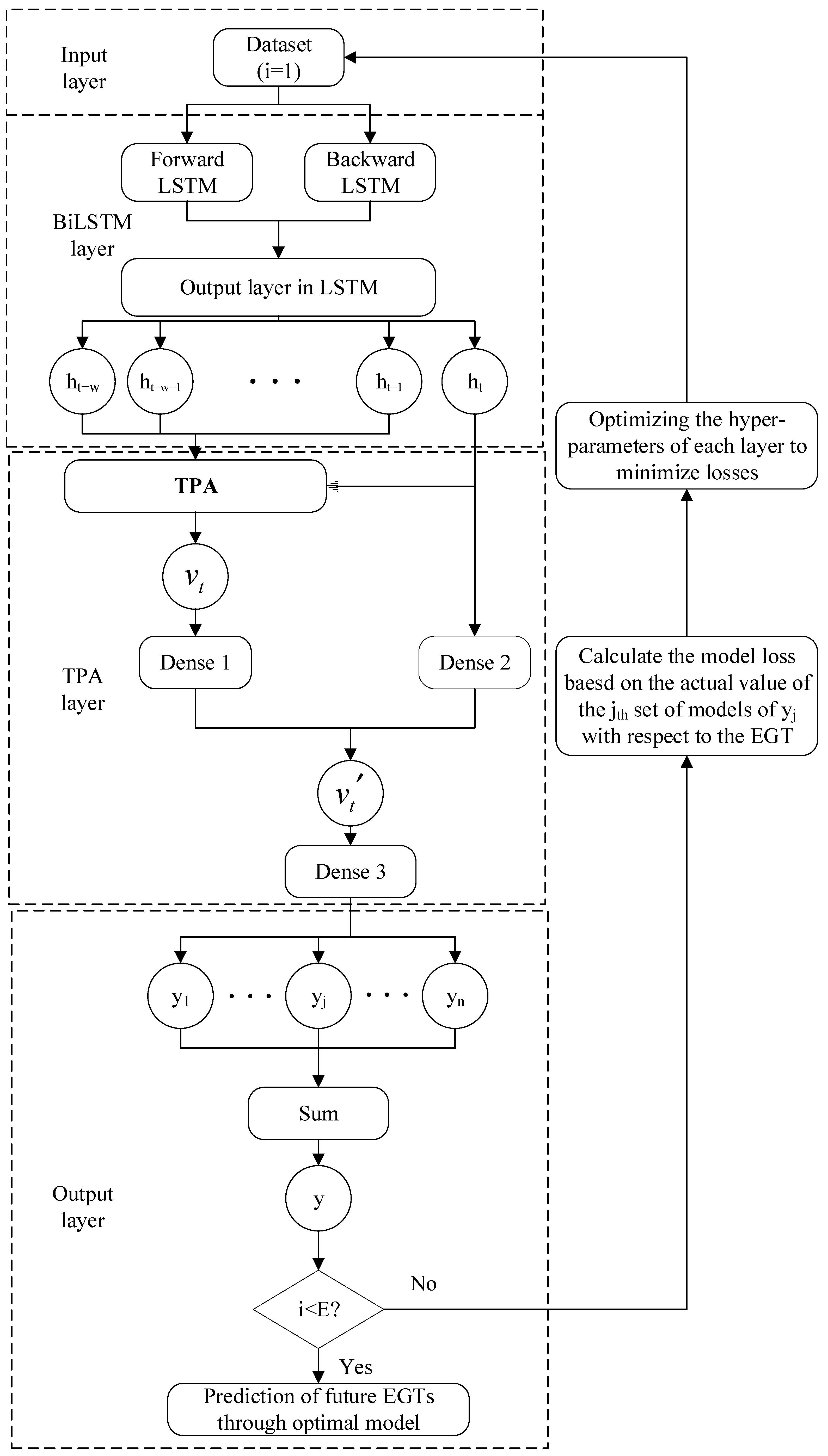
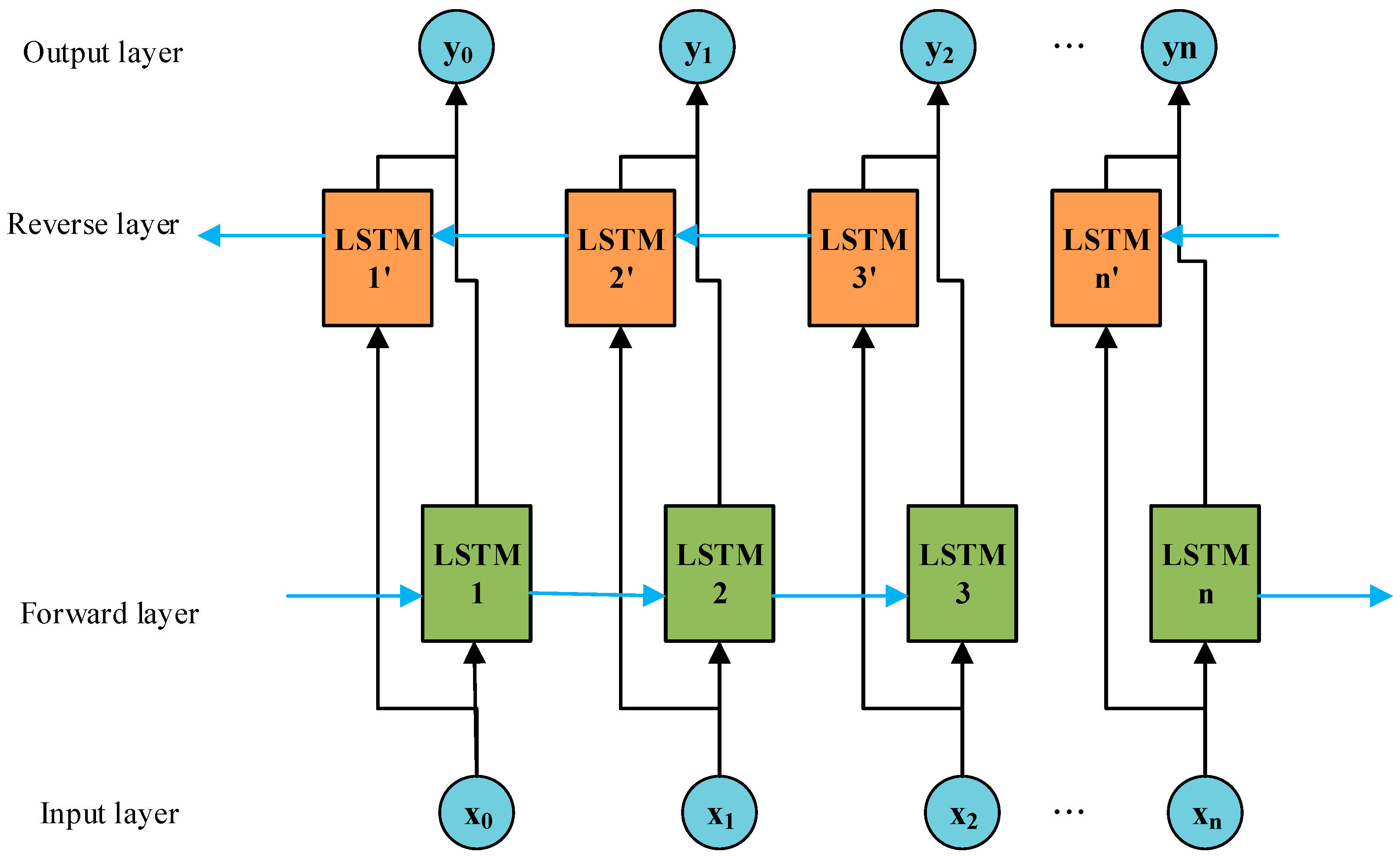
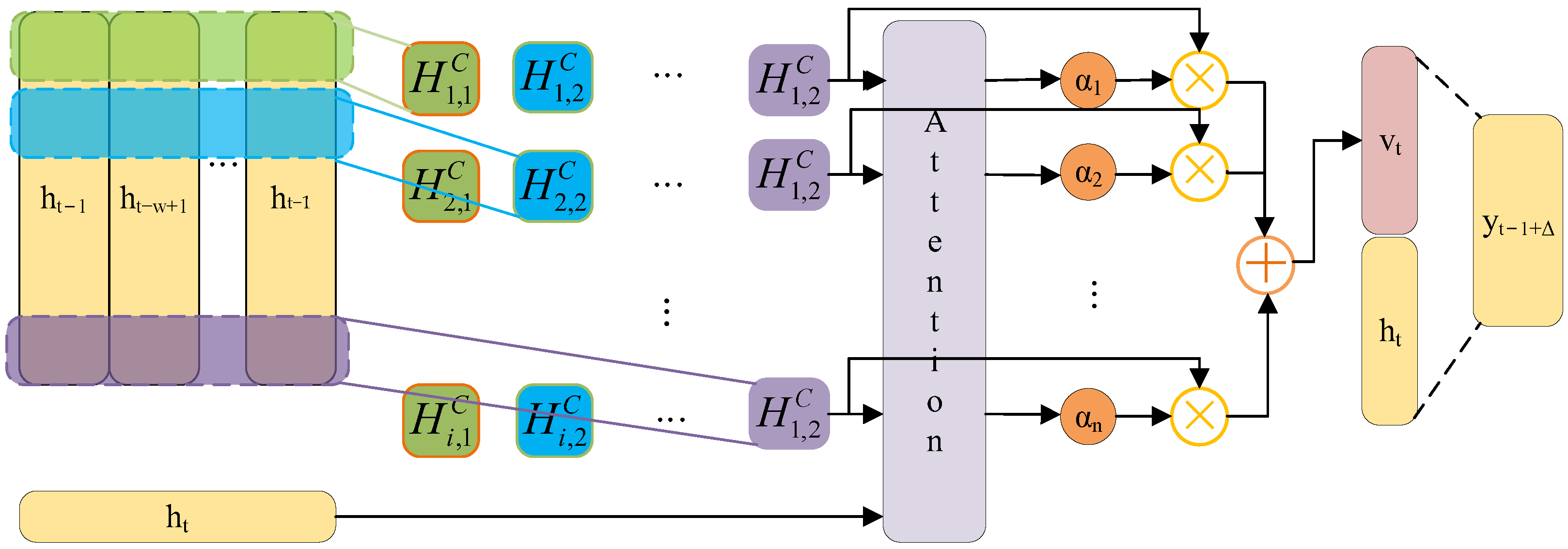
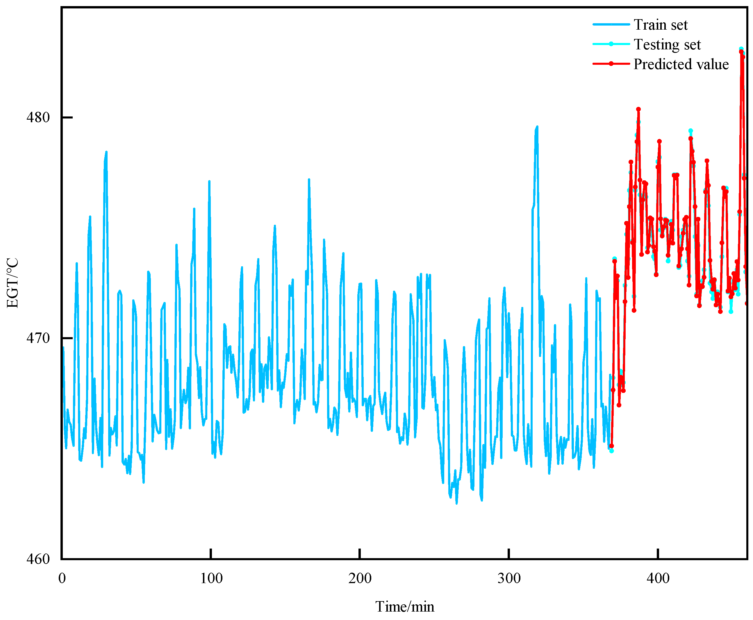
The EGT of MDE is a classic time series, characterized by continuity, volatility, and randomness in the variation patterns. When predicting short-term EGT trends, the current temperature value is closely related to the information from preceding and succeeding time periods. Therefore, this paper adopts the BiLSTM network as the foundational model for short-term EGT trend prediction to facilitate bidirectional interaction of data. On this basis, introducing the TPA mechanism helps to capture the interdependencies among multidimensional variable sequences at different time periods. Additionally, by utilizing an ISMA to find the optimal hyperparameter configuration in the BiLSTM network, the prediction model’s overall efficiency and the ability to generalize are significantly improved.

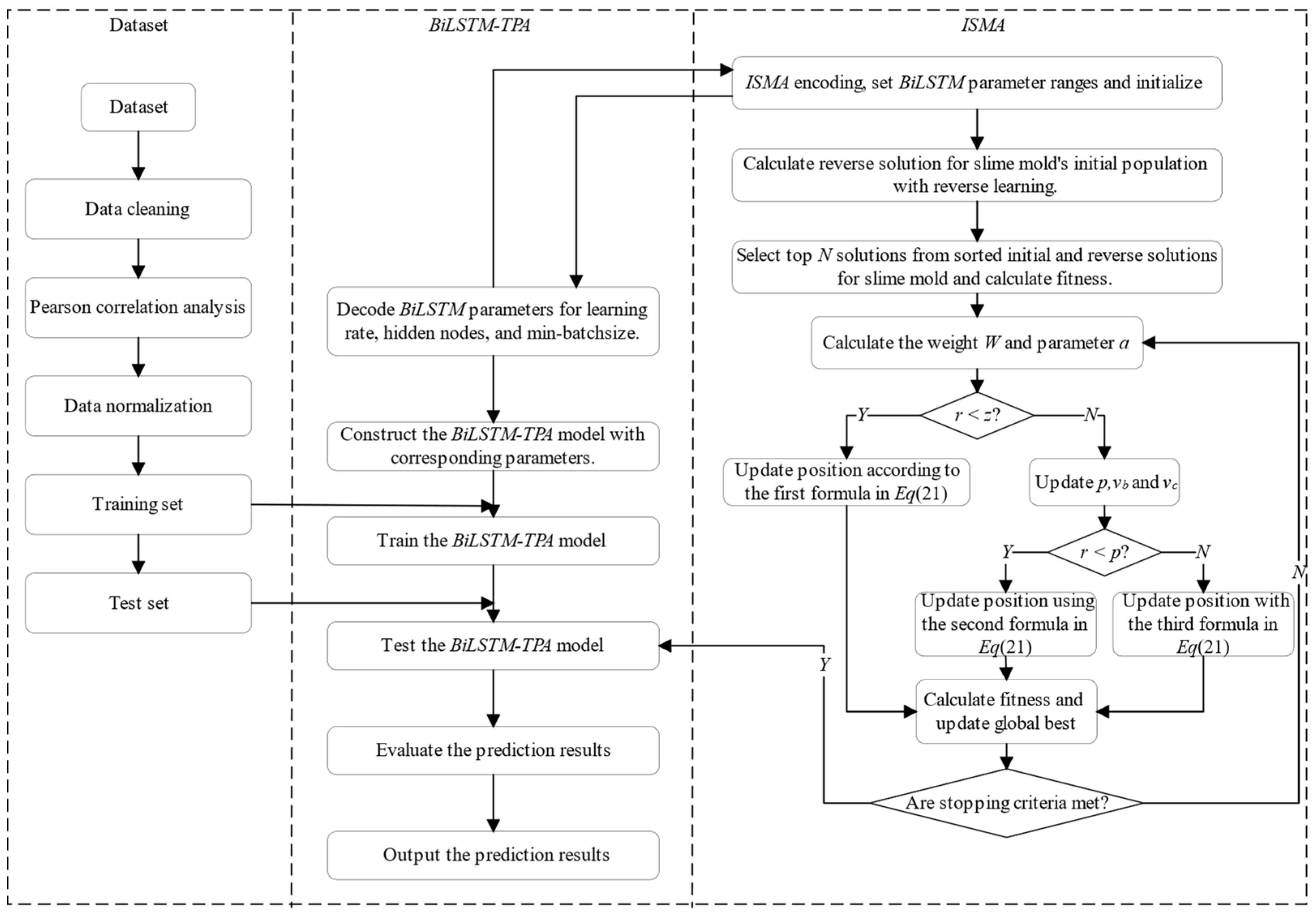
The traditional BiLSTM-TPA prediction model employs an empirical method to conduct multiple experiments for adjusting the network model’s hyperparameters, aiming to achieve the desired prediction accuracy. However, the model (as detailed in Figure 5) has a complex internal structure, contains numerous hyperparameters. Manually adjusting hyperparameters through trial and error introduces a significant workload and may impact the accuracy of prediction results. Therefore, this study introduces the ISMA to optimize the hyperparameters in the BiLSTM-TPA network, with the complete optimization process illustrated in Figure 6. The comprehensive algorithm consists of five main modules: input, ISMA, BiLSTM, TPA, and output. The input module performs data cleaning on the data collected by the shipboard monitoring system, then selects features related to the EGT through PCA to be used as the experimental dataset. In the BiLSTM module, decode the relevant hyperparameters according to the principles of the ISMA to obtain the number of nodes in each hidden layer, the min-batchsize, and the learning rate. the TPA module is responsible for weighted processing of the results from the hidden layers. The output module is responsible for generating the final prediction results, calculating the RMSE value between the actual and predicted values, and passing it back to the ISMA module as the fitness value. The ISMA module adjusts the position of the slime mold population based on the fitness value, achieving population updates and a global optimal search, ultimately obtaining a set of optimized hyperparameters.

3.1. Optimization of the BiLSTM-TPA Prediction Model Based on the ISMA

This study incorporates the ISMA for hyperparameter optimization within the BiLSTM network mode. Initially, establish the value boundaries for the hyperparameters within the BiLSTM network model. Subsequently, the BiLSTM module decodes the hyperparameters passed in by the ISMA to obtain and the number of nodes in each hidden layer, the min-batchsize, learning rate. Following this, the prediction model is trained and learned, calculating the root mean square error (RMSE) between the predicted EGT values and actual EGT values. Then, this RMSE value is relayed back to the ISMA module to serve as a fitness value, allowing the adjustment of the population members’ positions according to this current fitness value in the pursuit of the global optimal solution. Ultimately, a set of optimized hyperparameters is obtained. 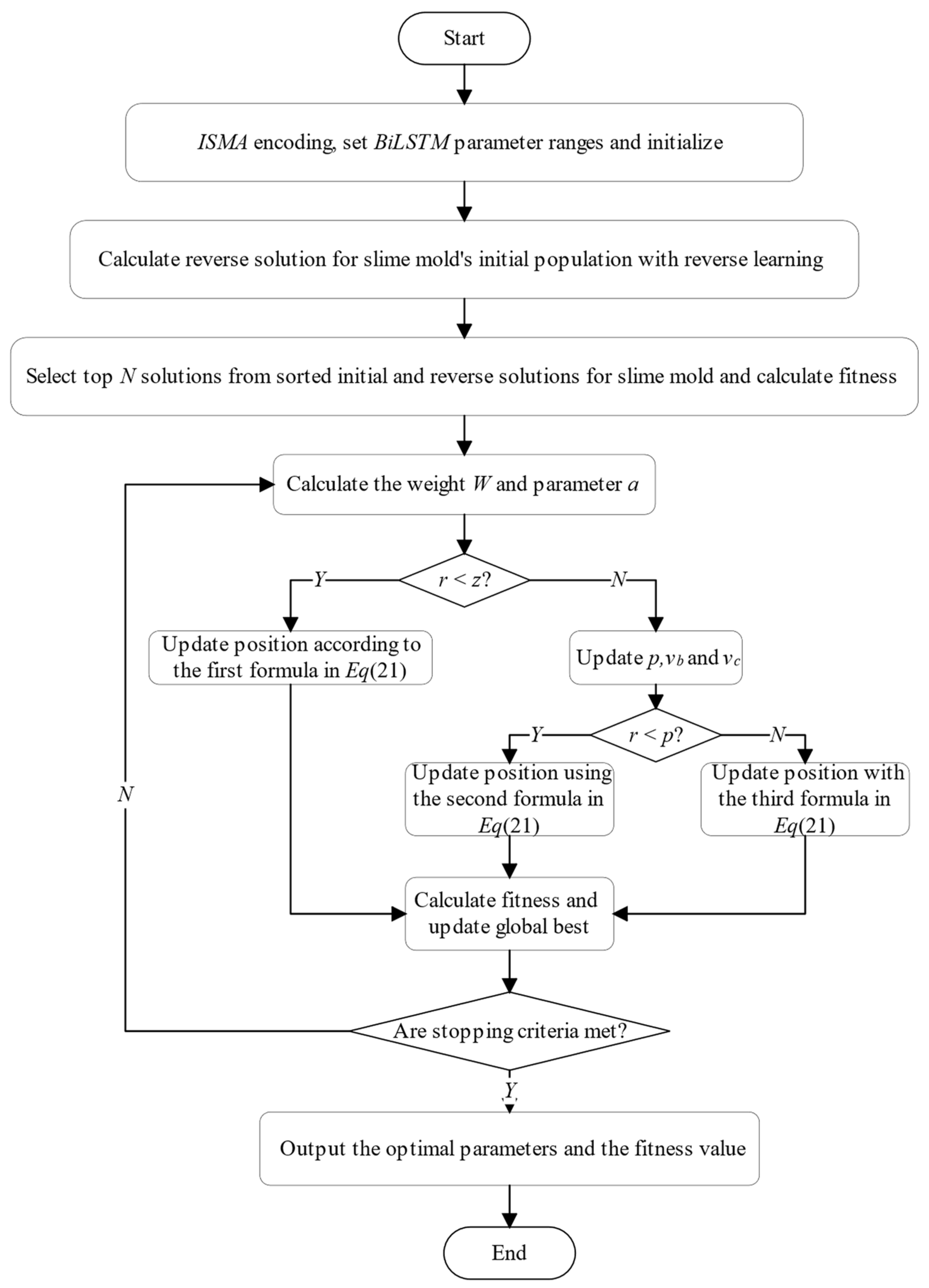Figure 7 illustrates the ISMA, with the comprehensive steps for calculation detailed as follows.

• Step 1: Determine the range of values for the hyperparameters of the BiLSTM module.
• Step 2: Initialize parameters for the ISMA, including the search dimension (D), population size (N), and maximum number of iterations (t_max). Randomly generate initial slime mold population individuals, ensuring that the position of each slime mold individual corresponds to a combination of hyperparameters of the BiLSTM model.
• Step 3: Follow the reverse learning strategy to calculate the reverse solution for the initial population, and comprehensively evaluate the current solutions and reverse solutions. By merging the better-fit 50% of current solutions and 50% of reverse solution individuals, form the initial population for the ISMA.
• Step 4: Determine the initial fitness value of the slime mold population.
• Step 5: Calculate the parameter (a) and the weight (W).
• Step 6: Produce a random number (r) and contrast (r) with parameter (z). Should r be smaller than z, refresh the position of the individual based on the initial equation in Equation (21). If not, proceed to adjust p, v_b, and v_c further Contrast r with parameter p; should r be lower than p, revise the individual’s location using the second equation in Equation (21); otherwise, continue with the modification as per the third equation in Equation (21).
• Step 7: Recalculate the fitness of slime mold population individuals, and update the global optimum.
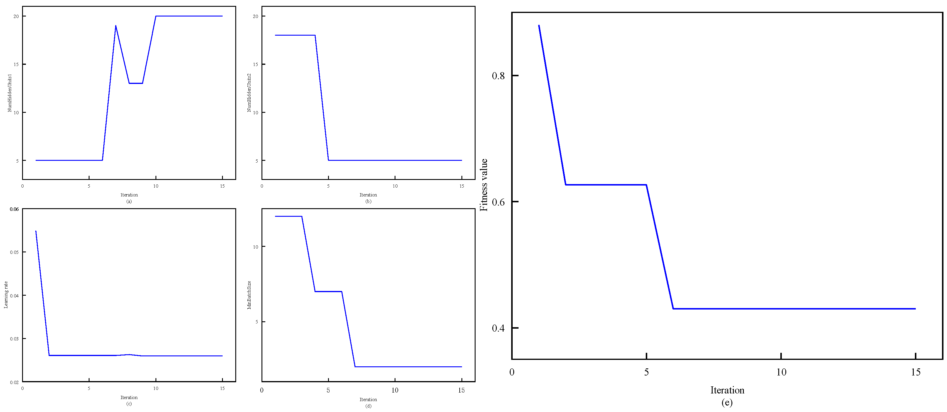
• Step 8: Check if the algorithm meets the termination condition. If it does, output the global optimum solution, which corresponds to the optimal parameters of the BiLSTM model. (the number of nodes in each hidden layer, min-batchsize, learning rate); if not, repeat Steps 5 to 8.

3.2. The Evaluation Index

The effectiveness of the EGT prediction algorithm for MDE largely depends on the accuracy of the trend prediction model. The higher the prediction accuracy, the greater its significance for guiding intelligent operation and maintenance of the ship’s engine room. To objectively evaluate the accuracy of the prediction results, it is necessary to establish corresponding evaluation indicators to verify the effectiveness and feasibility of the proposed experimental method. This paper aims to adopt the mean square error (MSE), the mean absolute percentage error (MAPE), the coefficient of determination (R²), and RMSE as the evaluation index for assessing the accuracy of predictions [37,38]. The specific calculation equations are as follows:

$$E_{MSE}=\frac{1}{n}{\displaystyle \sum _{i=1}^n{\left(\widehat{y_i}-y_i\right)}^2}$$

(22)

$$E_{MAPE}=\frac{1}{n}{\displaystyle \sum _{i=1}^n\left|\frac{y_i-\widehat{y_i}}{y_i}\right|}·100\%$$

(23)

$$E_{RMSE}=\sqrt{\frac{1}{n}{\displaystyle \sum _{i=1}^n{\left(y_i-\widehat{y_i}\right)}^2}}$$

(24)

$$E_{R^2}=1-\frac{{{\displaystyle {\sum }_{1=1}^n\left(\widehat{y_i}-{\overline{y}}_i\right)}}^2}{{\displaystyle {\sum }_{1=1}^n{\left(y_i-{\overline{y}}_i\right)}^2}}$$

(25)

In the equation, $y=[y_1,y_2,\dots ,y_i]$ and $\widehat{y}=\left[{\widehat{y}}_1,{\widehat{y}}_2,\dots ,{\widehat{y}}_i\right]$. It denotes the measured value sequence of the EGT in the ship-end monitoring system and the output sequence of the predicted value of the prediction model, respectively.

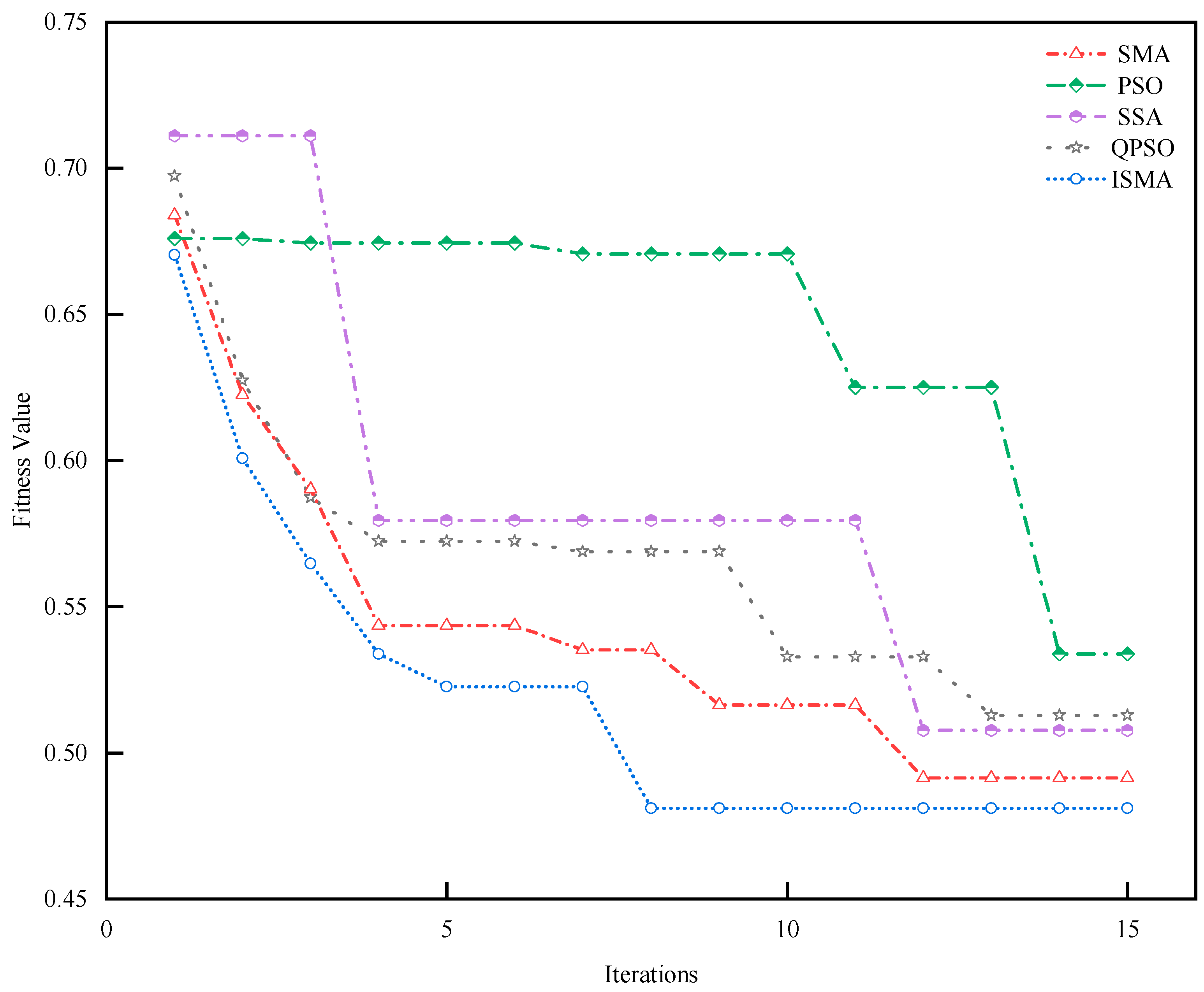
To verify the effectiveness of the short-term EGT trend prediction method proposed in this paper, this study introduces several prediction models, including the BiLSTM, BiLSTM-AT, BiLSTM-TPA, SMA-BiLSTM-AT, ISMA-BiLSTM-AT, and QPSO-BiLSTM-AT, and this study compared the outcomes of these models with those of the method proposed in this paper.

3.3. Experimental Configuration

The configuration of the experimental environment is shown in

Table 2. Experimental environment configuration table.

Experimental Configuration
Experimental platform	Matlab 2022b
Operating system	Window11 64-bit
CPU	AMD Ryzen 7 6800 H with Radeon Graphics 3.20 GHz
Running memory	16 G
Running language	C++

.

4. Discuss

This study conducts a predictive analysis on the shipboard historical operating data of the No. 2 dual-fuel engine of a certain liquefied natural gas bunkering vessel from 16 May 2018, to 18 May 2018. The No. 2 engine of this ship is a 6L34DF marine four-stroke engine produced by Wartsila, and the relevant parameters of this model’s MDE are shown in

Table 3. Engine parameters.

Parameters	Values
Engine type	Four strokes
Cylinder configuration	Inline 6 cylinders
Cylinder bore (mm)	340
Stroke (mm)	400
Compression ratio	12.6
Speed (r/min)	750
Power (kW)	2700

. Thermal parameters related to the EGT are extracted from the shipboard monitoring system of the 6L34DF. By performing PCA on the extracted thermal parameters, the original input feature sequence for the predictive model is obtained. The experimental approach introduced in this document is utilized for the calculation learning of the neural network model, and the resulting predictions are compared with those of other models to verify the effectiveness of the experimental method.

4.1. Input Feature Selection and Data Preprocessing

Before beginning the input features selection and data preprocessing, it is necessary to extract the historical operating data from the shipboard monitoring system of the 6L34DF type MDE. By consulting the relevant literature, input feature parameters related to the EGT are selected, as shown in

Table 4. Feature parameters before correlation analysis.

Parameters	Abbreviation
Exhaust Gas Temperature	EGT
Exhaust Gas Before T/C Temperature	EGTBTC
Exhaust Gas After T/C Temperature	EGTATC
Load	L
M/E Speed	MES
Scavenge Air Temperature	SAT
Supercharger Speed	SCS
Fuel Oil Pressure	FOP
Scavenge Air Pressure	SAP
Fuel Oil Temperature	FOT
Lubricating Oil Pressure	LOP
Oil Filter Inlet and Outlet Pressure Difference	OFPD

.

As is widely known, the EGT of MDE is a continuous dynamic thermodynamic parameter, influenced by multiple characteristic parameters within the subsystems. Therefore, when selecting features related to the EGT, their correlation with the EGT should be considered. However, selecting redundant features with weak correlation to the EGT during the input feature selection process may increase the model’s complexity, reduce the ability to adapt to new data, and lead to issues such as overfitting. Based on this, the method described in Section 2.1 is used to analyze the original dataset, resulting in the calculation of correlation coefficients between parameters (see Figure 8). According to the results of the correlation coefficient calculation, selecting feature parameters with absolute values greater than 0.4 for the prediction model’s input (refer to

Table 5. Results after correlation analysis.

Parameters	Abbreviation
Exhaust Gas Temperature	EGT
Exhaust Gas Before T/C Temperature	EGTBTC
Load	L
Supercharger Speed	SCS
Fuel Oil Pressure	FOP
Scavenge Air Pressure	SAP
Fuel Oil Temperature	FOT

), and select 460 sets of data from these feature parameters for experimental validation. Of these, the first 368 sets are used for model training, while the remaining 92 sets are used for testing the model. Meanwhile, to remove the impact of dimensional disparities among various feature parameters on the model’s predictive accuracy, normalize the input feature sequence of the original dataset to be between 0 and 1. The normalization calculation equation is shown in Equation (26) [39]:

$$x^{\prime }=a+\frac{x-x_{\min }}{x_{\max }-x_{\min }}\left(b-a\right)$$

(26)

wherein x′ denotes the normalized data; x, x_max and x_min, respectively, denote the original data, the maximum value in the original data, and the minimum value in the original data; a and b stand for the minimum and maximum values after normalization, respectively. In this experiment, a = −1 and b = 1.

4.2. Optimize Parameter Setting

To enhance the accuracy of the prediction, it is necessary to configure the network hyperparameters in a reasonable and effective manner before executing the prediction model. Through in-depth learning of the BiLSTM model, it is recognized that the hyperparameters influencing model performance encompass the quantity of layers in the hidden layer, batch size, quantity of training epochs, number of nodes within the hidden layer, learning rate, and the size of batch training, among other factors. This experiment decided to set the number of layers in the hidden layer to two to achieve fitting of arbitrary functions. Meanwhile, when determining the number of nodes in the hidden layer, it is necessary to balance different factors. Selecting an excessive number of nodes in the hidden layer can raise calculation complexity and potentially cause the model to become ensnared in local optimal solutions. conversely, too few nodes may lead to poor learning and training effects and weaker overall generalization ability. Therefore, it is necessary to carefully select the number of hidden layer nodes in the model design to maintain a balance between calculation efficiency and model performance. The batch size of the model determines the size into which the input sequence is segmented in the temporal dimension, and choosing the right batch size is a key factor in optimizing model performance. The setting of the number of training epochs should also be cautious; too many training epochs increase the burden on the model, and the batch training size should not be too large to avoid overfitting. Given the actual data volume, this experiment set the batch training size to 16. Additionally, as a sensitive parameter, the learning rate determines the iteration step size of the weights, and the selection requires reasonable setting within a region of minimal loss. Therefore, this study conducted optimization of the number of nodes in the hidden layer, min-batchSize, and learning rate in the BiLSTM model using the ISMA, with the range of parameter settings detailed in

Table 6. Setting of model network parameters range and population parameters.

Parameters	Setting Range
numHiddenUnits1	[5, 20]
numHiddenUnits2	[5, 20]
Min-BatchSize	[2, 16]
Learning rate	[0.001, 0.1]
Dropout	Adam
Optimizer	200
Epoch	2
Number of hidden layers	Sizepop = 20, Iterations = 15
ISMA optimization algorithm-related parameters	Search dimension: dim = 4 Search speed limit [−2, 2]

.

4.3. Analysis of Short-Term Exhaust Gas Temperature Trend Prediction Results for the 6L34DF

To confirm the effectiveness of the short-term EGT trend prediction model introduced in this paper, the outcomes of the predictions will be analyzed in detail from the following three aspects.

4.3.1. Comparative Analysis of the Convergence Characteristics of Combined Model Optimization Algorithms

To validate the superiority of the ISMA in the hyperparameter search of BiLSTM-TPA, we introduce Quantum Particle Swarm Optimization (QPSO), Particle Swarm Optimization (PSO), the Sparrow Search Algorithm (SSA) and SMA optimization algorithms to fine-tune the hyperparameters of the BiLSTM-AT network, and analyze them as comparative experiments. In this study, we set the same initial values for the five optimization algorithms and choose the loss function utilized in the training of the BiLSTM-AT network as the fitness function to assess the hyperparameter optimization capabilities of the three algorithms. The results are shown in Figure 9.

The fitness function curves for the QPSO, SMA, PSO, SSA, and ISMA optimization algorithms shown in Figure 9 are obtained by averaging the results after multiple hyperparameter optimization attempts, hence they possess a high level of credibility. By observing the convergence characteristics of the fitness functions for the three algorithms in the figure, it is evident that the ISMA successfully escapes the local optimum area after the seventh iteration, causing the fitness function to reach a state of convergence. The SMA, QPSO, PSO and SSA optimization algorithms achieve convergence after the 12th, 13th, 12th and 14th iterations, respectively, and both fall into local optimum areas, exhibiting a slower iteration speed. A comprehensive analysis indicates that, compared to the other four optimization algorithms, the ISMA has outstanding hyperparameter optimization performance.

4.3.2. Combination Model Optimization

To assess the efficiency of the ISMA for the hyperparameters of the BiLSTM-TPA network, update the positions and velocities of the slime molds during each iteration of the ISMA, and calculate the fitness value under the global optimal value. Through this process, the optimization results for each hyperparameter and their corresponding fitness values can be obtained. This section selects the ISMA-BiLSTM-TPA model performing the EGT trend prediction task in a certain round, where the ISMA optimizes the hyperparameters of the BiLSTM-TPA network and carries out an in-depth analysis of the optimization results. According to the optimization results displayed in Figure 10, as the count of ISMA iterations grows, the fitness value decreases incrementally as the position of the updated myxomycetes is adjusted, and after six iterations, the fitness value stabilizes, eventually converging on the optimal solution. The optimization using the ISMA produces optimal values for the quantity of nodes in the first and second hidden layers, the min-batchsize, and learning rate. As demonstrated by the results depicts in Figure 10e, the fitness value of the ISMA begins to converge after the sixth iteration and finally stabilizes at 0.429, indicating a rapid convergence speed of the ISMA. Figure 10a shows the change in the number of nodes in the first hidden layer as the number of iterations increases, eventually converging to 20; Figure 10b depicts the variation in the quantity of nodes in the second hidden layer with the rise in the number of iterations, eventually converging to 5; Figure 10c displays the adjustment in the learning rate corresponding to the increment in the number of iterations, eventually converging to 0.0257; Figure 10d illustrates the evolution of the min-batchsize with increasing iterations, eventually converging to 2. In summary, the ISMA demonstrates a rapid convergence speed when optimizing the BiLSTM-TPA prediction model.

4.3.3. Comparison of Prediction Effects of Combined Models

During the operation of MDEs, the EGT is affected by various factors, exhibiting a certain degree of fluctuation and significant uncertainty. The BiLSTM-TPA model possesses both short-term and long-term memory capabilities, and the TPA mechanism effectively captures the interrelationships between different time steps, thereby improving the model’s predictive accuracy. Consequently, this study selects BiLSTM as the fundamental framework and introduces the AT mechanism and TPA mechanism. Based on BiLSTM-AT and BiLSTM-TPA, QPSO, SMA, PSO, SSA and ISMA optimization algorithms are incorporated to optimize the results of short-term trend prediction for the EGT of MDEs, with the trend prediction results shown in Figure 11.

From Figure 11, it can be observed that the single model BiLSTM performs well in the initial prediction phase, but as time progresses, there is a significant deviation between the predicted results and the actual values. After introducing the AT mechanism and the TPA mechanism, although the prediction accuracy has improved, there is still a deviation phenomenon. This is because BiLSTM adopts a step-by-step prediction method, which leads to poor prediction performance. By introducing swarm intelligence optimization algorithms to optimize BiLSTM, the prediction performance of the BiLSTM-AT network is significantly improved, approaching the actual values. However, when there is a sudden change in the EGT, there is still a deviation in the prediction. After constructing the ISMA-BiLSTM-TPA combination model, the ISMA further optimizes the network model by increasing the number of initial solutions and enhancing the global search capability, thereby enhancing the stability. Meanwhile, the combination of the TPA mechanism to capture the features between each time step significantly improves the prediction accuracy of the model, making the predicted values of the proposed method closer to the actual values, and achieving the desired prediction effect. Figure 12 shows the prediction results of the ISMA-BiLSTM-TPA model.

The analysis of Figure 12 reveals that the EGT trend predictions made using the ISMA-BiLSTM-TPA model are highly consistent with the actual values in the test dataset. This result not only indicates the model’s accuracy in forecasting EGT trends but also reflects its sensitivity and responsiveness to changes in temperature trends. Through this sensitive reaction capability, the ISMA-BiLSTM-TPA model can effectively capture the subtle dynamics of temperature changes, providing strong support for temperature trend prediction. Therefore, the ISMA-BiLSTM-TPA model is not only innovative in theory but has also shown its significant value in practical applications, offering new approaches and methods for future applications and research in a broader field.

4.3.4. Comparison of Prediction Accuracy of Combined Models

Table 7. Comparison of prediction accuracy.

Dataset	Model	MSE/°C	MAPE/%	RMSE/°C	R2/%
Training	BiLSTM	9.5084	0.6394	3.0427	86.3%
	BiLSTM-AT	1.2485	0.2457	2.4637	89.4%
	BiLSTM-TPA	1.1529	0.2361	1.6732	90.2%
	SMA-BiLSTM-AT	0.9372	0.1402	1.2845	94.7%
	PSO-BiLSTM-AT	0.8033	0.1384	1.2483	95.3%
	SSA-BiLSTM-AT	0.6055	0.1228	0.3104	95.5%
	QPSO-BiLSTM-AT	0.5796	0.1187	0.2826	96.2%
	ISMA-BiLSTM-AT	0.2712	0.0453	0.2669	98.9%
	ISMA-BiLSTM-TPA	0.0232	0.0392	0.2302	99.6%
Testing	BiLSTM	37.3586	1.1899	6.1122	81.3%
	BiLSTM-AT	8.5204	0.5715	2.9190	86.4%
	BiLSTM-TPA	3.3852	0.2755	1.8393	88.5%
	SMA-BiLSTM-AT	1.1618	0.1716	1.7796	90.8%
	PSO-BiLSTM-AT	1.5772	0.1568	1.4983	91.7%
	SSA-BiLSTM-AT	1.5986	0.1602	1.5367	91.2%
	QPSO-BiLSTM-AT	1.6052	0.1209	1.2675	92.5%
	ISMA-BiLSTM-AT	0.6482	0.1234	0.8051	95.8%
	ISMA-BiLSTM-TPA	0.4284	0.1076	0.6545	98.2%

presents the performance evaluation indexes of various models during the training and testing phases. The analysis of the data in Table 7 reveals that the predictive performance of all models is generally higher during the training phase than in the testing phase. Notably, the ISMA-BiLSTM-TPA model demonstrates the best performance both in the training and testing phases. This section provides a detailed analysis of the performance of each prediction model during the testing phase as follows: Compared to other prediction models, the ISMA-BiLSTM-TPA model shows the most significant reduction in the MSE metric, with decreases of 36.9302, 8.0956, 2.9568, 0.7334, 1.1488, 1.1704, 1.1768, and 0.4284, respectively; in terms of MAPE, its values are reduced to 1.0823%, 0.4639%, 0.1679%, 0.084%, 0.0492%, 0.0506%, 0.1133%, and 0.0158%, respectively; the RMSE values are correspondingly reduced to 5.6775, 2.2645, 1.1848, 0.4234, 0.8438, 0.8822, 0.6130, and 0.1506; simultaneously, the R² values increased by 16.9%, 11.8%, 9.70%, 7.4%, 6.5%, 7.0%, 5.7%, and 2.4% compared to other models, respectively. This comprehensive analysis clearly indicates that the ISMA-BiLSTM-TPA model significantly surpasses other comparison models in accuracy and predictive performance, highlighting its strong capability and potential application in handling complex prediction tasks.

To confirm the practicality and effectiveness of the TPA mechanism in short-term EGT trend prediction under identical conditions, we additionally compared the predictive performance of the BiLSTM-AT model with the BiLSTM-TPA model. The results show that, compared to the BiLSTM-AT, the BiLSTM model incorporating the TPA mechanism exhibited reductions in MSE, MAPE, RMSE, and an increase in R² by 5.1388, 0.2960%, 1.0797, and 2.1%, respectively. Once again, these results demonstrate that the BiLSTM model with the TPA mechanism achieves higher prediction accuracy compared to the BiLSTM model with the AT mechanism.

According to the evaluation results of the ISMA-BiLSTM-AT, SMA-BiLSTM-AT, and BiLSTM-AT prediction models, the BiLSTM-AT prediction models based on the ISMA and SMA showed significant advantages in prediction accuracy. The MSE, MAPE, and RMSE values are notably lower compared to those from the sole use of the BiLSTM-AT model, with the R² also exhibiting a significant increase. This outcome emphasizes the stability and applicability of the SMA in time-series prediction. Further comparison of the evaluation metrics between the ISMA-BiLSTM-AT and SMA-BiLSTM-AT models validated the more effective optimization performance of the ISMA compared to the SMA.

The comprehensive analysis presented in this study demonstrates that the proposed ISMA-BiLSTM-TPA model exhibits outstanding practicality and stability, excelling in meeting the accuracy requirements of short-term EGT trend prediction tasks. By incorporating the ISMA strategy and the BiLSTM-TPA architecture, the model significantly enhances the predictive capability for time-series data, enabling it to accurately capture minute changes in EGT trends, thereby ensuring high precision and reliability of the prediction results.

5. Conclusions

This paper proposes a method for short-term EGT trend prediction in MDE based on an ISMA, to optimize the BiLSTM model under the TPA mechanism.

(1)

Using PCA, input feature parameters for the trend prediction model are selected based on the absolute value of the correlation coefficient between the EGT and other parameters, ensuring it exceeds 0.4 to avoid redundant features and minimize noise interference. Concurrently, employing the BiLSTM network to extract time-series features enhances the prediction accuracy of the EGT.

(2)

Introducing the TPA mechanism, crucial features between internal matrices of BiLSTM network hidden layers are extracted through the internal convolutional kernel. The TPA mechanism captures inherent connections between different input vectors and time steps, extracting relevant information more efficiently than traditional AT mechanisms, further improving the accuracy of the prediction model.

(3)

Introducing a reverse learning strategy and a nonlinear inertia weight decay strategy to the original SMA, the ISMA is developed, which improves the quality of the initial solution and the search capability of the SMA optimization algorithm. Comparing the optimization effects of the ISMA with the QPSO algorithm, it is proved that the ISMA has better optimization effects and higher prediction accuracy in the trend prediction task described in this paper.

The prediction results indicate that the ISMA-BiLSTM-TPA prediction model possesses better network parameter optimization capability and higher prediction accuracy in the prediction task, effectively improving the accuracy of short-term EGT trend prediction. Compared to other prediction models in this paper, this prediction model exhibits good applicability and stability for short-term EGT trend prediction tasks.

Despite this study providing valuable insights into the prediction of the EGT for MDEs, it faces several limitations. Firstly, the collection of input feature parameters related to the EGT of MDEs is limited, and the method has not been validated across different engine models due to the lack of parameters from other models. Moreover, the variety of optimization algorithms introduced is limited, constraining the universality of the method. Considering these limitations, future research will focus on expanding the dimensionality of input feature parameters and increasing the variety of optimization algorithms to further enhance the accuracy and applicability of the prediction method.

References

1. Zhong, G.Q.; Wang, H.Y.; Zhang, K.Y.; Jia, B.Z. Fault diagnosis of Marine diesel engine based on deep belief network. In Proceedings of the 2019 Chinese Automation Congress (CAC2019), Hangzhou, China, 22–24 November 2019; pp. 3415–3419. [Google Scholar]
2. Ehlers, T.; Portier, M.; Thoma, D. Automation of maritime shipping for more safety and environmental protection. AT-Automatisierungstechnik 2022, 70, 406–410. [Google Scholar] [CrossRef]
3. Gharib, H.; Kovács, G. A Review of Prognostic and Health Management (PHM) Methods and Limitations for Marine Diesel Engines: New Research Directions. Machines 2023, 11, 695. [Google Scholar] [CrossRef]
4. Liu, B.; Gan, H.B.; Chen, D.; Shu, Z.P. Research on Fault Early Warning of Marine Diesel Engine Based on CNN-BiGRU. J. Mar. Sci. Eng. 2023, 11, 56. [Google Scholar] [CrossRef]
5. Guo, Y.; Zhang, J.D. Fault Diagnosis of Marine Diesel Engines under Partial Set and Cross Working Conditions Based on Transfer Learning. J. Mar. Sci. Eng. 2023, 11, 1527. [Google Scholar] [CrossRef]
6. Feng, S.S.; Chen, Z.J.; Guan, Q.S.; Yue, J.T.; Xia, C.Y. Grey Relational Analysis-Based Fault Prediction for Watercraft Equipment. Front. Phys. 2022, 10, 885768. [Google Scholar] [CrossRef]
7. Gao, Z.L.; Jiang, Z.N.; Zhang, J.J. Identification of power output of diesel engine by analysis of the vibration signal. Meas. Control 2019, 52, 1371–1381. [Google Scholar] [CrossRef]
8. Zhang, Y.F.; Liu, P.P.; He, X.; Jiang, Y.P. A prediction method for exhaust gas temperature of marine diesel engine based on LSTM. In Proceedings of the 2020 IEEE 2nd International Conference on Civil Aviation Safety and Information Technology (ICCASIT), Weihai, China, 14–16 October 2020; pp. 49–52. [Google Scholar]
9. Hong, C.W.; Kim, J. Exhaust Temperature Prediction for Gas Turbine Performance Estimation by Using Deep Learning. J. Electr. Eng. Technol. 2023, 18, 3117–3125. [Google Scholar] [CrossRef]
10. Kumar, A.; Srivastava, A.; Goel, N.; McMaster, J. Exhaust Gas Temperature Data Prediction by Autoregressive MODELS. In Proceedings of the 2015 IEEE 28th Canadian Conference on Electrical and Computer Engineering (CCECE), Halifax, NS, Canada, 3–6 May 2015; pp. 976–981. [Google Scholar]
11. Zhang, B.S.; Zhang, L.; Zhang, B.; Yang, B.F.; Zhao, Y.C. A Fault Prediction Model of Adaptive Fuzzy Neural Network for Optimal Membership Function. IEEE Access 2020, 8, 101061–101067. [Google Scholar] [CrossRef]
12. Caliwag, A.; Han, S.Y.; Park, K.J.; Lim, W. Deep-Learning-Based Fault Occurrence Prediction of Public Trains in South Korea. Transp. Res. Rec. 2022, 2676, 710–718. [Google Scholar] [CrossRef]
13. Hoy, Z.X.; Phuang, Z.X.; Farooque, A.A.; Fan, Y.V.; Woon, K.S. Municipal solid waste management for low-carbon transition: A systematic review of artificial neural network applications for trend prediction. Environ. Pollut. (Barking Essex 1987) 2024, 344, 123386. [Google Scholar] [CrossRef]
14. Liu, B.Y.; Guangyao, O.Y.; Chang, H.B. A study on performance prediction of diesel engine based on the vibration measurement. In Proceedings of the ICEMI 2005: Conference Proceedings of the Seventh International Conference on Electronic Measurement & Instruments, Beijing, China, 16–18 August 2005; Volume 5, pp. 157–160. [Google Scholar]
15. Cui, L.X.; Huo, H.B.; Xie, G.H.; Xu, J.X.; Kuang, X.H.; Dong, Z.P. Long-Term Degradation Trend Prediction and Remaining Useful Life Estimation for Solid Oxide Fuel Cells. Sustainability 2022, 14, 9069. [Google Scholar] [CrossRef]
16. Wang, Y.H.; Xiao, Z.H.; Liu, D.; Chen, J.B.; Liu, D.; Hu, X. Degradation Trend Prediction of Hydropower Units Based on a Comprehensive Deterioration Index and LSTM. Energies 2022, 15, 6273. [Google Scholar] [CrossRef]
17. Theerthagiri, P.; Ruby, A.U. Seasonal learning based ARIMA algorithm for prediction of Brent oil Price trends. Multimed. Tools Appl. 2023, 82, 24485–24504. [Google Scholar] [CrossRef]
18. Xu, D.Y.; Ren, L.; Zhang, X.Y. Predicting Multidimensional Environmental Factor Trends in Greenhouse Microclimates Using a Hybrid Ensemble Approach. J. Sens. 2023, 2023, 6486940. [Google Scholar] [CrossRef]
19. Zhao, G.; Li, S.L.; Zuo, W.Q.; Song, H.R.; Zhu, H.P.; Hu, W.J. State trend prediction of hydropower units under different working conditions based on parameter adaptive support vector regression machine modeling. J. Power Electron. 2023, 23, 1422–1435. [Google Scholar] [CrossRef]
20. Li, D.Y.; Zhou, F.H.; Gao, Y.T.; Yang, K.; Gao, H.M. Power plant turbine power trend prediction based on continuous prediction and online oil monitoring data of deep learning. Tribol. Int. 2024, 191, 109083. [Google Scholar] [CrossRef]
21. Liu, Y.; Gan, H.B.; Cong, Y.J.; Hu, G.T. Research on fault prediction of marine diesel engine based on attention-LSTM. Proc. Inst. Mech. Eng. Part M-J. Eng. Marit. Environ. 2023, 237, 508–519. [Google Scholar] [CrossRef]
22. Li, D.Z.; Peng, J.B.; He, D.W. Aero-Engine Exhaust Gas Temperature Prediction Based on Lightgbm Optimized by Improved Bat Algorithm. Therm. Sci. 2021, 25, 845–858. [Google Scholar] [CrossRef]
23. Huang, D.R.; Deng, Z.P.; Wan, S.H.; Mi, B.; Liu, Y. Identification and Prediction of Urban Traffic Congestion via Cyber-Physical Link Optimization. IEEE Access 2018, 6, 63268–63278. [Google Scholar] [CrossRef]
24. Yang, C.C. Correlation coefficient evaluation for the fuzzy interval data. J. Bus. Res. 2016, 69, 2138–2144. [Google Scholar] [CrossRef]
25. Xue, X.M.; Zhou, J.Z. A hybrid fault diagnosis approach based on mixed-domain state features for rotating machinery. ISA Trans. 2017, 66, 284–295. [Google Scholar] [CrossRef]
26. Lu, W.J.; Li, J.Z.; Wang, J.Y.; Qin, L.L. A CNN-BiLSTM-AM method for stock price prediction. Neural Comput. Appl. 2021, 33, 4741–4753. [Google Scholar] [CrossRef]
27. Kim, J.; An, Y.; Kim, J. Improving Speech Emotion Recognition Through Focus and Calibration Attention Mechanisms. In Proceedings of the Interspeech 2022, Incheon, Republic of Korea, 18–22 September 2022; pp. 136–140. [Google Scholar]
28. Yao, M.; Min, Z. Summary of Fine-Grained Image Recognition Based on Attention Mechanism. In Proceedings of the Thirteenth International Conference on Graphics and Image Processing (ICGIP 2021), Kunming, China, 16 February 2022. [Google Scholar]
29. Liu, J.J.; Yang, J.K.; Liu, K.X.; Xu, L.Y. Ocean Current Prediction Using the Weighted Pure Attention Mechanism. J. Mar. Sci. Eng. 2022, 10, 592. [Google Scholar] [CrossRef]
30. Shih, S.Y.; Sun, F.K.; Lee, H.Y. Temporal pattern attention for multivariate time series forecasting. Mach. Learn. 2019, 108, 1421–1441. [Google Scholar] [CrossRef]
31. Gharehchopogh, F.S.; Ucan, A.; Ibrikci, T.; Arasteh, B.; Isik, G. Slime Mould Algorithm: A Comprehensive Survey of Its Variants and Applications. Arch. Comput. Methods Eng. 2023, 30, 2683–2723. [Google Scholar] [CrossRef]
32. An, G.Q.; Chen, L.B.; Tan, J.X.; Jiang, Z.Y.; Li, Z.; Sun, H.X. Ultra-short-term wind power prediction based on PVMD-ESMA-DELM. Energy Rep. 2022, 8, 8574–8588. [Google Scholar] [CrossRef]
33. Ewees, A.A.; Al-qaness, M.A.A.; Abualigah, L.; Algamal, Z.Y.; Oliva, D.; Yousri, D.; Abd Elaziz, M. Enhanced feature selection technique using slime mould algorithm: A case study on chemical data. Neural Comput. Appl. 2023, 35, 3307–3324. [Google Scholar] [CrossRef] [PubMed]
34. Zhang, X.S.; Liu, X.J.; Li, J.H. A Novel Method for Battery SOC Estimation Based on Slime Mould Algorithm Optimizing Neural Network under the Condition of Low Battery SOC Value. Electronics 2023, 12, 3924. [Google Scholar] [CrossRef]
35. Tizhoosh, H.R. Opposition-based learning: A new scheme for machine intelligence. In Proceedings of the International Conference on Computational Intelligence for Modelling, Control & Automation Jointly with International Conference on Intelligent Agents, Web Technologies & Internet Commerce, Vienna, Austria, 28–30 November 2005; Volume 1, pp. 695–701. [Google Scholar]
36. Wu, Z.S.; Fu, W.P.; Xue, R. Nonlinear Inertia Weighted Teaching-Learning-Based Optimization for Solving Global Optimization Problem. Comput. Intell. Neurosci. 2015, 2015, 292576. [Google Scholar] [CrossRef]
37. Li, G.H.; Zhang, S.L.; Yang, H. A Deep Learning Prediction Model Based on Extreme-Point Symmetric Mode Decomposition and Cluster Analysis. Math. Probl. Eng. 2017, 2017, 8513652. [Google Scholar] [CrossRef]
38. Lian, L. Network traffic prediction model based on linear and nonlinear model combination. ETRI J. 2023. [Google Scholar] [CrossRef]
39. Tan, Y.H.; Niu, C.Y.; Tian, H.; Hou, L.S.; Zhang, J.D. A one-class SVM based approach for condition-based maintenance of a naval propulsion plant with limited labeled data. Ocean Eng. 2019, 193, 106592. [Google Scholar] [CrossRef]
Figure 1. LSTM Network Structure.
Jmse 12 00541 g001
Figure 2. BiLSTM Network Architecture Diagram.
Jmse 12 00541 g002
Figure 3. The Structure of TPA.
Jmse 12 00541 g003
Figure 4. Any Solution and Its Reverse Solution.
Jmse 12 00541 g004
Figure 5. BiLSTM-TPA Model Structure.
Jmse 12 00541 g005
Figure 6. Forecasting Process.
Jmse 12 00541 g006
Figure 7. ISMA Optimization Process.
Jmse 12 00541 g007
Figure 8. The PCC Obtained after Calculation.
Jmse 12 00541 g008
Figure 9. Optimization Algorithm Fitness Curve.
Jmse 12 00541 g009
Figure 10. ISMA-BiLSTM-TPA Optimal Parameters. (a) Optimization results of the number of nodes in the first hidden layer (b) Optimization results of the number of nodes in the second hidden layer (c) Optimization results of the learning rate (d) Optimization of the min-batchsize (e) Fitness function of the ISMA algorithm.
Jmse 12 00541 g010
Figure 11. Comparison Chart of Trend Prediction Results.
Jmse 12 00541 g011
Figure 12. Prediction Results of the ISMA-BiLSTM-TPA Model.
Jmse 12 00541 g012