Article

A Prescriptive Model for Failure Analysis in Ship Machinery Monitoring Using Generative Adversarial Networks

1
Maritime Transportation Engineering PhD Program, Istanbul Technical University, 34940 Istanbul, Turkey
2
Department of Basic Science, Istanbul Technical University, 34940 Istanbul, Turkey
3
Industrial Data Analytics and Decision Support Systems Center, Azerbaijan State University of Economics (UNEC), Baku AZ1001, Azerbaijan
*
Author to whom correspondence should be addressed.
J. Mar. Sci. Eng. 2024, 12(3), 493; https://doi.org/10.3390/jmse12030493
Submission received: 8 February 2024 / Revised: 25 February 2024 / Accepted: 27 February 2024 / Published: 15 March 2024

Abstract

:
In recent years, advanced methods and smart solutions have been investigated for the safe, secure, and environmentally friendly operation of ships. Since data acquisition capabilities have improved, data processing has become of great importance for ship operators. In this study, we introduce a novel approach to ship machinery monitoring, employing generative adversarial networks (GANs) augmented with failure mode and effect analysis (FMEA), to address a spectrum of failure modes in diesel generators. GANs are emerging unsupervised deep learning models known for their ability to generate realistic samples that are used to amplify a number of failures within training datasets. Our model specifically targets critical failure modes, such as mechanical wear and tear on turbochargers and fuel injection system failures, which can have environmental effects, providing a comprehensive framework for anomaly detection. By integrating FMEA into our GAN model, we do not stop at detecting these failures; we also enable timely interventions and improvements in operational efficiency in the maritime industry. This methodology not only boosts the reliability of diesel generators, but also sets a precedent for prescriptive maintenance approaches in the maritime industry. The model was demonstrated with real-time data, including 33 features, gathered from a diesel generator installed on a 310,000 DWT oil tanker. The developed algorithm provides high-accuracy results, achieving 83.13% accuracy. The final model demonstrates a precision score of 36.91%, a recall score of 83.47%, and an F1 score of 51.18%. The model strikes a balance between precision and recall in order to eliminate operational drift and enables potential early action in identified positive cases. This study contributes to managing operational excellence in tanker ship fleets. Furthermore, this study could be expanded to enhance the current functionalities of engine health management software products.

1. Introduction

The International Maritime Organization (IMO), the global standard-setting authority for the maritime industry, has increased scrutiny of ships’ environmental performance. The IMO added a new annex to the International Convention for the Prevention of Pollution from Ships (MARPOL) in 1997, with a focus on minimizing airborne emissions from ships, mainly from sulfur oxides (SOx), nitrogen oxides (NOx), ozone-depleting substances (ODSs), and volatile organic compounds (VOCs), which began being enforced on 19 May 2005. Amendments made to MARPOL Annex VI in 2011 mandated technical and operational energy efficiency measures to reduce CO2 emissions from maritime shipping. These measures adopted by the IMO were the first global mandatory GHG reduction regime for international industry [1]. With the adoption of new amendments, emissions reductions have become the main focus of research by policymakers. The Energy Efficiency Design Index (EEDI) aimed to encourage the use of more energy-efficient machinery, thus lowering carbon emissions. Energy-saving devices (ESDs) have become standard applications for almost all newly constructed ships. In 2011, during the 72nd session of the Marine Environment Protection Committee, it was agreed to adopt the initial strategy for reducing GHG emissions from ships, with provisions to review this in 2023. The IMO’s initial target was focused on reducing CO2 emissions per transport work by 70% by 2050 compared with 2008, and reducing the total annual GHG emissions by 50% by 2050 compared with the 2008 baseline. The IMO’s initial strategy, aligned with the Paris Agreement, was a wake-up call for the industry as it highlighted that while ESDs will help operators to comply with regulations in the short term, they are not the only long-term solution for the decarbonization of the maritime industry. Various alternatives are currently being implemented or researched, such as hybrid propulsion systems and the full electrification of ships, as well as alternative fuels, such as methanol, ammonia, and hydrogen. However, the maturity level and applicability of these alternatives changes greatly based on the ship type and size. The quality of marine fuels is crucial for efficient combustion in ships’ main engines, auxiliary generators, and boilers. It is important to understand the physicochemical properties of the fuel bunkers. Studies show that under consistent cyclic conditions, fuel supply variations can impact efficiency by up to 5% [2]. Additionally, bunker analysis can provide guidance to ship operators when troubleshooting combustion-quality-related problems as well as combustion efficiency problems. While bunker samples are sent to laboratories for evaluation, it is also possible to carry out a multiparametric assessment of fuel quality results, which can be completed almost instantly [3]. On the other hand, one of the greatly varying factors in ship efficiency is operations. The carbon intensity indicator (CII) is a measure of a ship’s energy efficiency and is described as the grams of CO2 emitted per cargo-carrying capacity per nautical mile [4].
As expressed above, a couple of factors can be controlled to reduce the carbon intensity of maritime operations. Annual fuel consumption can be controlled by means of energy-saving devices (ESDs) and efficient operations. As the maritime industry adapts to environmental regulations, the fatigue resistance of ships’ mechanical components, such as propellers and engines, is becoming increasingly critical. The implementation of ESDs, as well as efficient operations such as slow steaming, is pivotal for reducing emissions, although it necessitates a thorough understanding of the fatigue behavior of these components under operational loads [5]. While it may seem easy, identifying inefficient operations and identifying anomalies requires a set of data, including normal and abnormal conditions. As the machinery operates within a certain operating range, it is not always easy to identify anomalies as they start to develop; most of the time, they only become evident when the equipment fails. Manufacturers set design ranges and alarm parameters, but those variables mainly focus on the safety aspect of machinery operation, so the efficiency of the machinery is considered secondary when designing the operating range for machinery. Similarly, machinery failures are fixed as soon as they are identified. Therefore, this introduces the problem of data imbalance. The data imbalance problem is frequently the bottleneck of performance classification. Data imbalance is the terminology used to describe the situation where the class distributions are not equal, i.e., when one class, which is called the majority class, far exceeds the other classes, which are called the minority classes. This is the case when different classes have a significantly different number of samples. Due to the data imbalance problem, the training algorithm gives more weight to the class(es) with the majority of samples, which results in biased classifiers. Despite its complexity, the algorithm’s prediction model needs a lot of data to understand the hidden data correlations for output prediction. This is attributed to the fact that the training of predictive algorithms relies on deciphering intricate patterns within historical data. The augmentation of data quantity corresponds to heightened precision in the predictive model.
This is where generative adversarial networks (GANs) have emerged as a groundbreaking solution, enabling the generation of synthetic data that closely resemble real-world data. The ability to generate synthetic data that accurately capture the underlying distribution and statistical properties of real data has significant implications. generative adversarial networks offer a powerful solution by employing a dual architecture of generator and discriminator networks, enabling the generation of synthetic data that are remarkably similar to real data. This paper explores the utilization of GANs in ship machinery anomaly detection by using synthetic data generation, highlighting their potential to overcome data limitations and foster innovation across ship machinery anomaly detection.
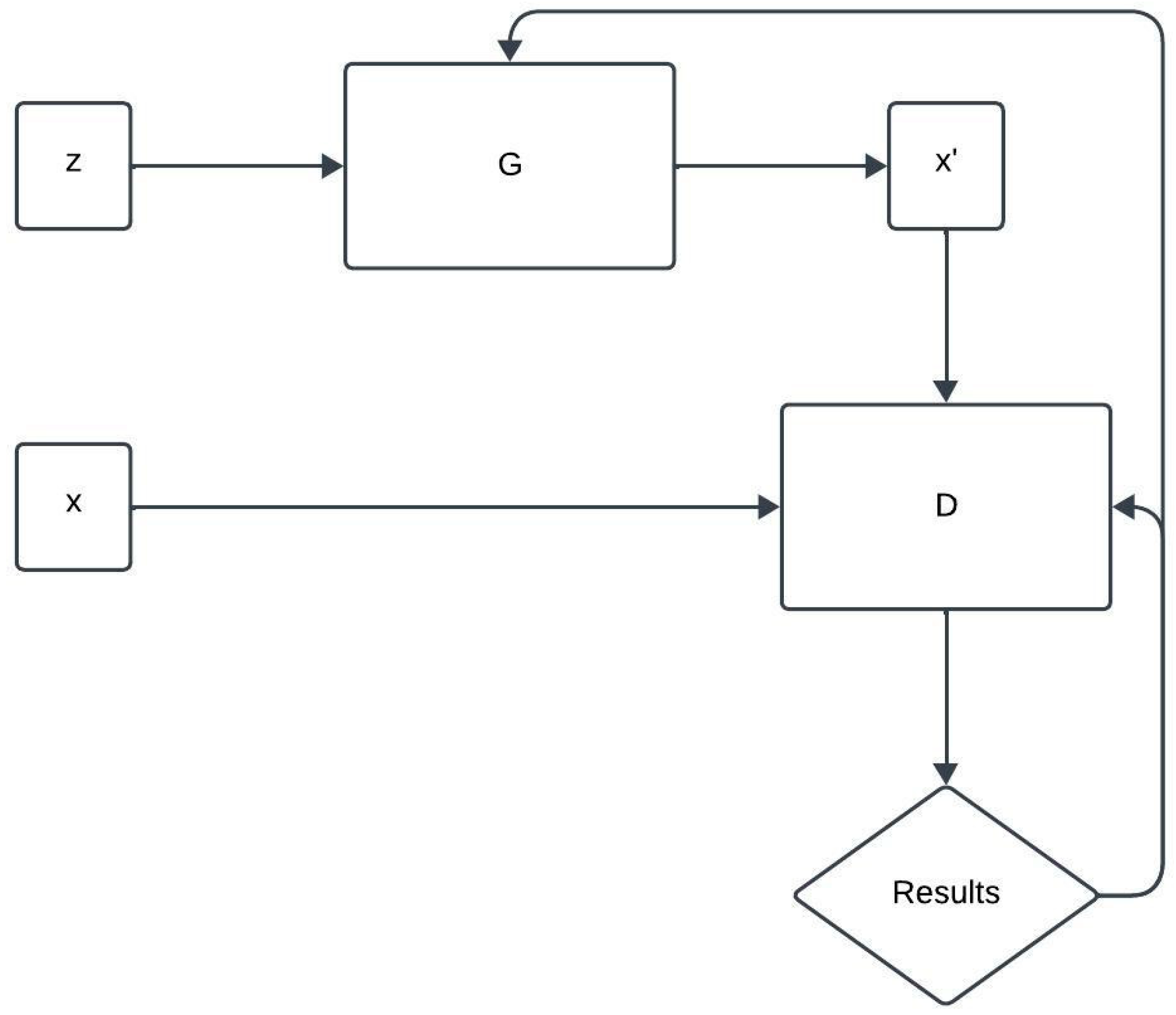
GANs are powerful algorithms that utilize a dual training process, comprising a generator and a discriminator. The generator’s objective is to generate synthetic images that exhibit a high degree of realism, resembling real images. The discriminator is trained to differentiate between the generated images and real images. As GANs have evolved, they have made significant progress in unconditional image synthesis, generating images without any specific conditioning. Different types of GANs are deployed for different applications: realistic image generation [6,7], natural language processing [8,9], healthcare and medical imaging [10], reinforcement learning [11], etc. The use of GANs has primarily focused on computer vision and image generation; however, GANs have emerged as a promising solution for the generation of synthetic tabular data that exhibit similar statistical characteristics and patterns to the original data.
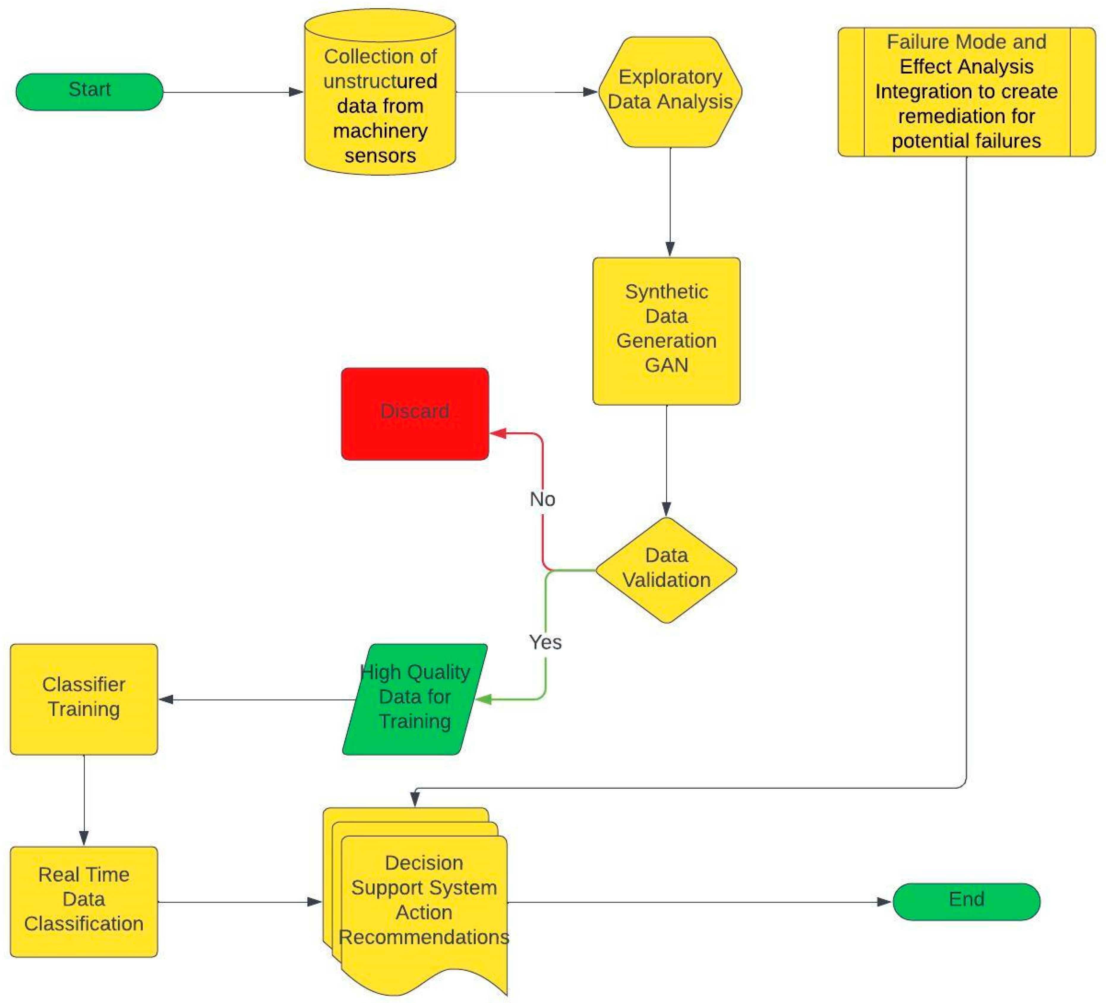
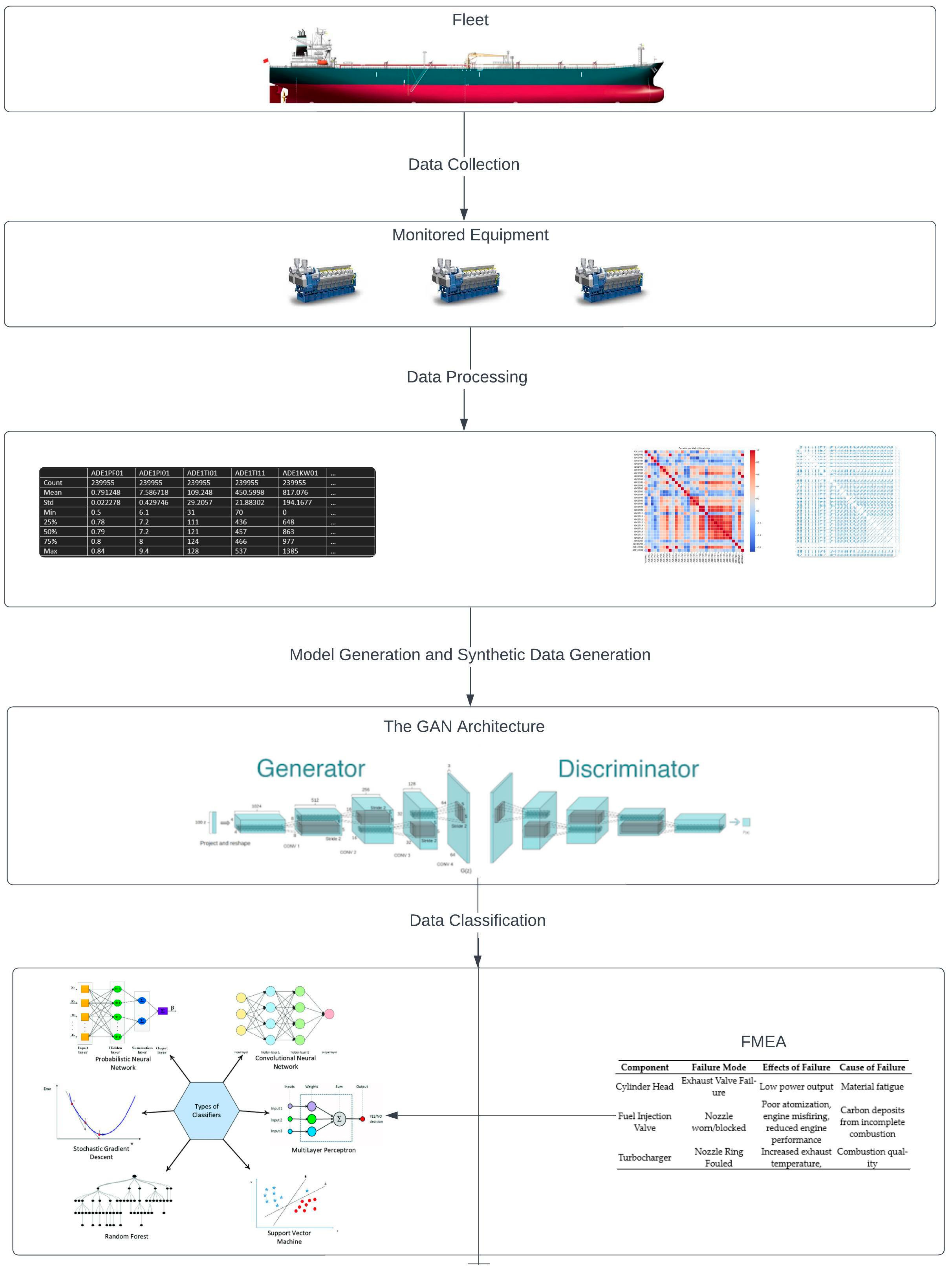
In this study, we focus on the prescriptive model of ship machinery monitoring based on GANs, supported by failure mode and effect analysis (FMEA) techniques. The proposed prescriptive model for ship machinery monitoring makes the following contributions to the literature.
First, generative adversarial networks have attracted significant attention and been applied to varying domains, including shipping. However, to the best of our knowledge, within the maritime domain, they are still not applied for machinery anomaly detection. GANs and their variants are used here for object detection and surveillance systems.
Second, data-driven approaches are integrated with FMEA for autonomous decision support systems (DSSs) for ship machinery systems.
Third, a comparison is made with six different classifiers trained with synthetic data and tested on real-life data for fault diagnosis. The model achieved 30–83% accuracy on real-life data for anomaly detection.
The rest of this study is organized as follows. In Section 2, anomaly detection in the maritime industry is discussed; in Section 3, the main tools used in this study, GAN and FMEA, are reviewed, followed by an explanation of the proposed prescriptive model. Section 4 details the results of this study, and in Section 5, the conclusions are discussed.

2. Literature Review

In recent years, data-driven approaches have garnered substantial attention in the maritime industry, a sector characterized by its historical significance and evolving technological landscape. The integration of advanced machine learning techniques, particularly in the realms of computer vision and natural language processing, has not only paralleled, but in some instances surpassed human performance in certain tasks [12]. This paradigm shift towards data-centric methodologies in maritime operations is indicative of a broader trend in industry and academia alike.
With the ever-growing complexity of marine systems, the increasing maintenance demand and complexity of troubleshooting increases the need for decision support systems. Investigation reports indicate that 80% of accidents are caused by human error [13].
The categorization of data-driven models into white, black, and gray box models offers a framework for understanding their applications and limitations [14]. White box models, known for their transparency and explainability, are grounded in clear, underlying mechanisms. White box models are widely used, as they are characterized by their explicit mathematical equations and parameters, which have real-world interpretations. They are commonly used in reliability analyses [15] and failure analyses [16].
In contrast, black box models operate on statistical inferences, deriving conclusions from input–output relationships without explicitly revealing their internal workings. With the growing implementation of IoT devices and increases in the availability and accessibility of data, black box models are gaining significant momentum. In the maritime industry, black box models and data-driven algorithms are employed across a diverse range of applications. These applications include the prediction of fuel consumption by the main engine [17], voyage optimization via vessel speed optimization [18], and the prognostics and health management of ship machinery systems [19]. Each of these applications’ predictive capabilities relies on data-driven models, which aim to enhance the ship’s operational efficiency and decision-making processes within the maritime sector. Gray box models represent a hybrid approach, enhancing the predictive capabilities of white box models by incorporating elements of black box models to address uncertainties. Gray box models, also called hybrid models, have gained attention as they aim to bridge the gap between white box models and black box models. They offer a valuable compromise between transparency and flexibility. By combining domain knowledge and data-driven insights, gray box models provide versatility and effectiveness to the predictive tools. They have been used for fuel consumption predictions [20], remaining useful life predictions [21], hull fouling predictions [22], and engine performance predictions [23].
Despite their advantages, a primary concern with the use of data-driven models in maritime applications is the autonomy of their decision-making. The reliance on purely data-driven methods can obscure the nuanced understanding that domain expertise provides. To bridge this gap, recent studies have advocated for a dual approach that synergizes data-driven techniques with domain knowledge [24,25,26]. This involves integrating expert insights into black box models to enhance their relevance and applicability in real-world maritime scenarios.
In the context of maritime operations, anomaly detection plays a pivotal role in ensuring safety, security, and efficiency. Recent advancements in this area have been significantly influenced by the integration of cutting-edge technologies. The Internet of Things (IoT) has revolutionized data collection in maritime environments, offering real-time monitoring capabilities. When combined with machine learning algorithms, devices can provide instantaneous anomaly detection.
The integration of advanced data-driven approaches in anomaly detection within the maritime industry marks a significant stride towards modernizing and securing maritime operations. However, the successful implementation of these technologies necessitates a balanced approach, addressing the challenges mentioned earlier. One of the main challenges with classification problems is the lack of labeled data for the anomaly class. Many of the anomaly detection capabilities are rule-based, such that simple rules trigger an alarm [27]. Additionally, the majority of diagnostics systems were found to rely on physics-based models [28] and predictive models’ targeting to minimize prediction errors, which the prediction results mostly ignored [29].
This study focuses on addressing the key challenges highlighted in anomaly detection in the maritime domain. The first problem we are tackling is the data imbalance problem via the implementation of GAN-based synthetic failure data generation. One of the primary methods used to address the imbalance in datasets is the use of various resampling techniques, such as undersampling, oversampling, and the synthetic minority oversampling technique (SMOTE) [30]. However, where anomalies are rare, GANs can generate realistic examples of these events by improving the model’s ability to detect them.
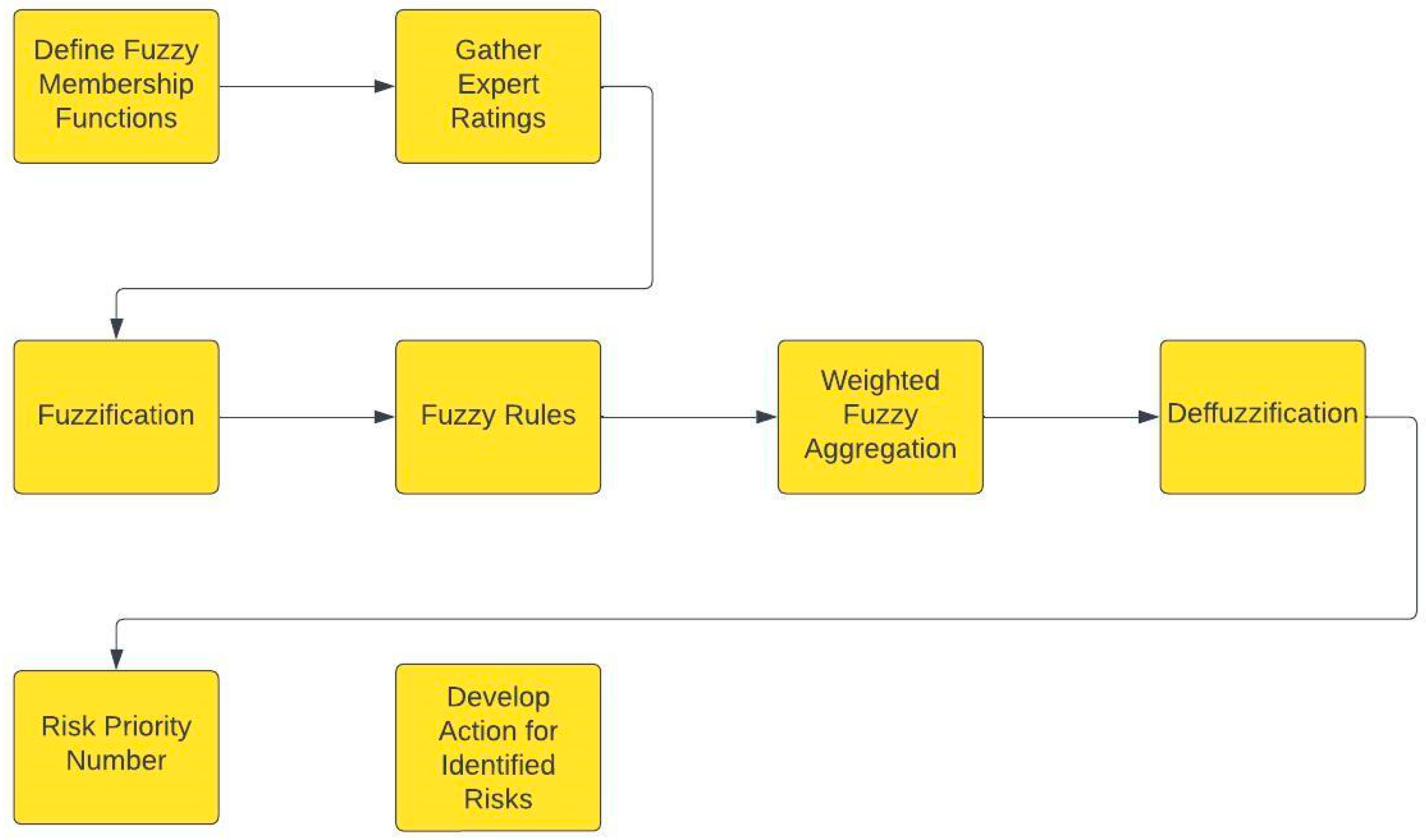
Secondly, in order to overcome the lack of recommendations in predictive systems, we are proposing an effective FMEA-based DSS that leverages the systematic identification and prioritization of potential failure modes to guide the decision-making process.

3. Methodology

3.1. FMEA

Failure mode and effect analysis (FMEA) is a systematic, structured approach used to identify, assess, and mitigate potential points of failure within a process or product design. The primary objective of this method is to proactively pinpoint and resolve issues that could lead to failures, with a focus on prevention rather than rectification. This approach significantly reduces downtime and enhances the overall reliability and safety of the manufacturing process across its entire lifecycle, from initial production to eventual service [31].
The origins of FMEA can be traced back to the 1940s, originating from the U.S. military, which published MIL-P-1629 in 1949 [32], marking its development as a methodical tool for failure analysis [33]. However, it was first notably adopted in 1963 during the Apollo space project, where it played a crucial role in ensuring the safety and reliability of the spacecraft and mission operations. Its use was initially more prevalent within military projects, where the stakes were exceptionally high.
The broader industrial adoption of FMEA, particularly in the automotive industry, gained momentum following notable incidents and the increasing demand for safety and quality assurance. A pivotal moment was its introduction by the Ford Motor Company in response to the Pinto affair. This incident highlighted the critical need for systematic safety and risk assessment methods in the automotive industry, leading to the widespread implementation of FMEA. It was used not just to enhance product safety, but also to comply with growing regulatory standards and public expectations for safer vehicles [34]. In 1994, certain manufacturers, called the Big Three (Chrysler, Ford, and General Motors), published updated rankings and clarifications. These efforts were presented in SAE J 1739, called “Potential Mode and Effects Analysis in Design and Potential Failure Mode and Effects Analysis in Manufacturing and Assembly Process Reference Manual” [35].
Since then, FMEA has evolved and been integrated into various industrial sectors, becoming a cornerstone of risk management and quality assurance practices. Its application extends beyond the automotive industry, encompassing sectors such as aerospace [36], healthcare [37], and electronics [38], where the identification and mitigation of potential failures are crucial for both safety and operational efficiency.
Risk evaluation is determined by the Risk Priority Number (RPN) within FMEA studies. This number is a product of the Occurrence, Severity and Detection values. The results of the exercise enable decision-makers to prioritize the determined failures and implement preventive measures to lower system risks [39]. In this study, we used the framework developed by the British Standards Institution, IEC 60812:2018 [40]. The risk severity indices adopted within this study are presented in Table 1, Table 2 and Table 3 [41,42].
In the process of conducting an FMEA for a marine auxiliary diesel generator, a specialized team of experts, as listed in Table 4, undertook a comprehensive review. This review encompassed both the system and subsystem levels of the diesel generator, ensuring a thorough understanding of all potential points of failure was obtained. The team’s approach was methodical, focusing on identifying and evaluating various failure modes that could impact the generator’s performance and reliability in marine environments.
A key aspect of this analysis involved the determination of the Risk Priority Number (RPN) for each identified failure mode. The RPN is a crucial metric in FMEA, quantifying the risk associated with each potential failure by considering its severity, occurrence likelihood, and detection difficulty. However, traditional FMEA is commonly criticized due to its drawbacks in practical applications [43]. Fuzzy FMEA stems from the need to address the uncertainties and subjective assessments often encountered in traditional FMEA. Fuzzy FMEA is widely used when dealing with qualitative and uncertain information [44,45,46,47]. We used linguistic expressions to evaluate the ratings and trapezoidal membership function derived from studies within the literature [48]; Table 5, Table 6 and Table 7 summarize the fuzzy scale developed [43] from the literature. Figure 1 represents the fuzzy FMEA process. Trapezoidal membership function is used thanks to its flexibility in representing phenomena with a clear range of full membership, while triangular functions are better suited to approximations or when data naturally cluster around a midpoint [49].
A trapezoidal fuzzy number is defined by four parameters (a, b, c, and d), where a and d are the “feet” of the trapezoid, representing the lowest and highest points where the membership function is greater than zero, and b and c are the shoulders of the trapezoid, representing the range where the membership function equals one.
By calculating the RPN, the team was able to prioritize the failure modes, focusing on those that posed the greatest risk and required immediate attention. To enhance the robustness of the FMEA, insights from the existing literature on marine diesel engines were integrated for analysis [31,50,51,52,53,54]. An excerpt of the FMEA is presented in Table 8.
The results obtained from the failure mode and effect analysis (FMEA) provide a critical foundation for formulating prescriptive actions to manage and mitigate risks, as well as serving as a crucial input for the development of machine learning algorithms, aiming to classify different types of failures.

3.2. GAN

An emerging method, generative adversarial networks (GANs), proposed by Goodfellow et al., consists of two neural networks, called the generator and discriminator. The generator is used to generate new samples by learning the underlying principles of the dataset and is used for the generation of new datasets, while the discriminator tries to categorize the generated data as real or false [55]. GANs have gained popularity in academia, as they were first used as a generative algorithm, providing results that were indistinguishable from the real data. The training process is often expressed as a minimax game, where the generator minimizes the probability of the discriminator being correct, and the discriminator minimizes the probability of making a mistake. The equilibrium of this game ideally results in the generator producing realistic samples that are indistinguishable from real data [56]. GANs have been successfully applied in various domains, including image synthesis [57], text-to-image synthesis [58], composing [59], and last but not least, anomaly detection [60].
The working architecture of this network is demonstrated in Figure 2.
The generator takes random noise as its input and generates synthetic data. While trying to create samples that are realistic, it learns to map random noise to data samples without having direct access to the real data. The generator is trained through its communication with the discriminator. The discriminator is a binary classifier that evaluates whether a given sample is real or fake; it acts as classifier for the generator’s output. Iterative and adversarial training processes are performed simultaneously for the generator and discriminator; as the generator improves, the discriminator must adapt to the increasingly realistic generated samples. The ideal optimization outcome is the Nash equilibrium, where the generator produces samples that capture the distribution of real samples [61].
The training of the GAN can be described as follows.
{x1, x2, x3, …, xn} represent the real-world data; z represents random noise input to the generator. At the start of each training iteration, the sampling of noise vector z takes place.
z i ~ N ( 0,1 )
Using the noise vector, the generator creates a batch of fake data:
G ( z i )
Concurrently, a batch of real data samples, xi, is drawn from the training dataset.
The discriminator is trained on the real data with the objective of correctly classifying them as real:
Loss for real data : log ( D x i )
where D represents the discriminator network.
The discriminator is also trained on the false data generated by the generator, with the goal of correctly classifying them as false.
Loss for fake data : log ( 1 D G z i )
The total loss for the discriminator is represented by the sum of the losses for real and false data, which is used to update the discriminator’s parameters.
L D = 1 m i = 1 m ( y i log D ( x i ) ) + ( 1 y i ) log ( 1 D G z i )
After updating the discriminator, the generator is trained with the goal of producing data that the discriminator classify as real.
L G = 1 m i = 1 m ( l o g ( D G z i )
The entire process is repeated iteratively until convergence criteria are met or predefined conditions are met, such as a certain number of epochs being completed.

3.3. Classification Models

3.3.1. Random Forests

Breiman proposed a machine learning algorithm: an ensemble of decision trees. It builds multiple decision trees and merges them together to obtain prediction results [62]. The Figure 3 presented below illustrates a typical representation of the Random Forest algorithm.

3.3.2. Decision Tree Classifier

Decision trees are non-parametric supervised learning methods that are generally used for classification and regression problems. A decision tree learns simple decision rules inferred from the data features. The model is represented as a tree, where each node represents a feature, each branch represents a decision rule, and each leaf node represents an outcome. The decision at each node splits the data into subsets based on the value threshold of the feature.

3.3.3. Logistic Regression

Logistic regression is a statistical model for analyzing data in which there are one or more independent variables that determine an outcome. The outcome is measured with a dichotomous variable. The logistic function can be described as follows [63]:
σ z = 1 1 + e z

3.3.4. AdaBoost Classifier

Adaptive Boosting is an ensemble technique that combines multiple weak learners to create a strong learner. It sequentially adjusts the weights of the training data, where more weight is given to misclassified instances at each iteration, causing the model to focus more on difficult cases. With dataset features given as X and labels represented by Y, each weak learner, ht, is assigned a weight:
α t = 1 2 ln ( 1 e r r o r t e r r o r t )
The final strong learner is a weighted combination of all weak learners:
F x = t = 1 T α t h t ( x )

3.3.5. K-Nearest Neighbors (KNN)

The k-nearest neighbors algorithm, based on the ‘k’ closest data, points to a given point in a dataset and makes predictions based on its neighbors [64]. In classification tasks, KNN assigns a class to the new data point based on the majority class of its ‘k’ nearest neighbors [65]. A mathematical representation of the algorithm can be expressed as follows:
d x , x = i = 1 n ( x i x i p ) 1 / p

3.3.6. Xtreme Gradient Boosting

The extreme gradient boosting method is an advanced implementation of the gradient boosting algorithm developed by Chen and Guestrin [66]. XGBoost improves upon the base gradient boosting algorithm through system optimization and provides model flexibility [67]. The ensemble model in XGBoost is defined as follows:
F x = k = 1 K F k ( x )

3.4. Proposed Methodology

3.4.1. Conceptual Framework

We propose an automated prescriptive framework that adopts a state-of-the-art generative adversarial network to address data imbalance problems when limited anomaly data are available. The use of GANs has been proposed by various studies [68,69,70]; however, the majority of existing studies only focus on the proportion of anomaly detection, whereas the novelty of our proposal comes from its prescriptive framework.
The model starts with data collection from ship machinery. With the rapid implementation of the IoT, the available sensory information from ship machinery increased exponentially. The number of data points can reach up to 3000 depending on the vessel type. Diesel generators play an essential role in ships, serving as the backbone for power generation on a vast array of vessels. Diesel generators supply electricity for auxiliary systems and accommodation, including navigation, communication, and safety systems; therefore, their reliability, fuel efficiency, and ability to operate under demanding conditions are essential. Figure 4 and Figure 5 present a conceptual framework and detailed flowchart of the model.

3.4.2. Data Description

In our case study, the dataset that we used was collected from a diesel generator installed on a 310,000 DWT oil tanker, and the data collection period was six months with 1 min intervals. The data collected from the diesel generator include 33 features directly related to the engine and engine subsystems. Vessel specification, principal information about the diesel generator, and the parameters selected for analysis are shown in Table 9, Table 10, and Table 11, respectively.

3.4.3. Exploratory Data Analysis

Data-driven methods involve working with the available data to obtain insights and build models; exploratory data analysis (EDA) and data preprocessing are inseparable steps in this process. EDA consists of in-depth statistical summaries, visualization techniques, and pattern recognition to determine the inherent characteristics of variables and the relationships between them. Statistical analytics during EDA, such as computing the central tendencies, dispersion, and correlation coefficients, provide quantitative insights into the dataset’s structure [71]. Data preprocessing addresses data quality issues. This involves employing techniques such as imputation for missing values, normalization or standardization techniques used for scaling the values of features, and the use of statistical methods that are less sensitive to the presence of outliers [72]. This framework ensures the reliability of the models that are built by addressing potential biases and outliers before the modelling steps start. Table 12 shows a summary of the statistical analysis of the dataset after the cleaning of data.
Data-driven methods predict the target variable by harnessing the variational relationship embedded in the dataset, which is often discerned through correlation analysis. This involves understanding and quantifying the associations between input features and output. Correlation analysis, typically using measures such as the Pearson correlation coefficient, is employed to reveal the strength and direction of the linear relationships between variables [73]. The iterative nature of data-driven models means that models are tuned based on the variational relationships discovered during the correlation analysis. Model tuning involves incorporating additional features, adjusting model parameters, or exploring different algorithms. A general outline of the study is illustrated in Figure 4, and the Pearson correlation analysis and strongest correlation variables are shown in Figure 6 and Figure 7, respectively. In order to maintain the diversity of the generated samples, the trade-off regarding high-dimensionality data and computational complexity was evaluated, and the decision was made to not to drop any features from the dataset.

4. Results and Discussion

The synthetic data that were generated resemble real data; then, the imbalanced dataset was classified according to the framework described in Section 3.4.1. The specifications of the device used for modelling were established with an Intel Core i7-13700F 2.10 GHz processor, 16 GB of RAM, NVIDIA GeForce RTX 4070, and 1TB SSD hard disk. During the modelling process, TensorFlow 2.10.0 was utilized within a Python 3.9.18 programming environment. In order to generate the synthetic data, various hyperparameter tuning operations were performed throughout the GAN modelling phase, where the model underwent significant changes in its performance as the training process evolved. The GAN architecture integrates a discriminator with a total of four layers (512, 256, 128, and 1) and a generator comprising three layers (1024, 2048, and 4096), employing LeakyReLU as the primary activation function, and using intermediate layers and sigmoid in the final layer of the discriminator. Table 13 and Table 14 summarize the key hyperparameters used during modeling. Additionally, during performance optimization, we implemented Python packages Cprofiler and Snakeviz to visualize the computation time of the algorithm. The final computational performance of the GAN architecture is demonstrated in Figure 8.
Synthetic data were generated and evaluated using various metrics before the best model for the GAN was chosen. These metrics included the discriminator’s accuracy when using real samples and generated samples, the F1 score, the precision score, and the recall score. Table 15 presents the accuracy of the discriminator using the GAN model at different epochs.
The discriminator’s accuracy when using real data remained strong throughout the iterations, whereas its accuracy when using generated samples fluctuated significantly; it achieved a perfect accuracy of 100%, which indicates that the model was overfitted. Based on the accuracy of the discriminator, 100 and 200 epochs stand out as the best performers. However, accuracy, as a traditional metric, might provide misleading results [74]. Therefore, an evaluation of additional metrics is required. In summary, the GAN model, at 100 epochs, achieves an F1 score of 67.18%, yielding the best results regarding the balance between precision and recall; thus, the GAN model with 100 epochs can be used for classification problems.
After the selection of the optimal GAN model, a comparative study was conducted to evaluate the performance of six different classifiers: AdaBoost, Random Forest, decision tree, Logistic Regression, KNN, and XGBoost. The performance of the classifiers in the classification algorithm was evaluated by several metrics, namely, accuracy, precision, recall, F1, and elements of the confusion matrix. These metrics offer a multifaceted view of each classifier’s performance, which is crucial for understanding their applicability to classification tasks. Table 16 presents a summary of the classification results, along with the metrics used for evaluation.
Based on a comparative study of six classification algorithms, XGBoost emerged as the best classification algorithm, with an accuracy of 83.13% and an F1 score of 51.18%. This also indicates the effectiveness of the XGBoost algorithm for varying data distributions. However, logistic regression displayed significant limitations, with an 80.41% recall rate, suggesting that, while it can identify the majority of positive instances, it had a high rate of misclassification. AdaBoost and KNN classification algorithms achieved respective accuracies 81.84% and 80.48%; the increased number of false positives indicates a potential trade-off when aiming to achieve high sensitivity. Random Forest and decision tree classifiers also had an increased false positive rate, which demonstrates the overfitting problem that can occur with a given dataset. This indicates the need for feature selection in order to improve the model’s generalization ability.

5. Conclusions

The growing data acquisition abilities are increasing the demand for data-driven methods; therefore, GAN studies are increasing exponentially. The implementation of GAN algorithms in the maritime domain is concentrated in the area of vessel trajectory prediction [75] and object detection [76]. This study presents a pioneering approach to ship machinery monitoring by integrating GAN with FMEA techniques. The classification with engineering approaches such as FMEA enhances the prescriptive abilities of the framework by providing treatment actions for the detected anomalies. Our model, validated using real-time data from a diesel generator on a 310,000 DWT oil tanker, demonstrates significant potential in enhancing the precision and recall of anomaly detection in maritime operations. The developed algorithm shows a high accuracy of 83.13% and achieves a balance between precision and recall, thus facilitating early operational interventions. The contributions of this research extend to ensuring operational excellence in tanker ship fleets, offering a novel pathway for the advancement of engine health management software products. Additionally, predictive tools require a significant amount of data in order to establish baseline conditions for machinery. Baseline data are used to understand the relationship between features and equipment behavior. However, the degradation of machinery is expected to occur over time; therefore, baselines for algorithms generally need to be adjusted over time. The implementation of the GAN models can significantly reduce the time required to establish baseline readings for machinery condition monitoring and enable operators to use these tools more efficiently. Similarly, when anomalies are experienced, they are immediately remedied. Thus, the availability of anomaly data is limited. One potential extension for this study is to strengthen existing engine health management software products by training the GAN model on the engine’s operational data. This integration could improve the accuracy and effectiveness of anomaly detection and failure monitoring systems. Lastly, even though it has been around for decades, the popularity of transfer learning has surged in recent years due to advancements in deep learning algorithms. A GAN model that is pre-trained on a dataset could be used for domain-specific regularization. One natural extension of this framework is the implementation of Multi-Criteria Decision Making (MCDM) methods. The use of methods such as the Preference Ranking Organization Method for Enrichment Evaluation (PROMETHEE) or Technique for Order of Preference by Similarity to Ideal Solution (TOPSIS) could enable operators to implement the best alternative from a set of alternatives based on their performance. Another potential extension to the proposed framework is the implementation of feature extraction algorithms such as Principal Component Analysis (PCA), which could be used to quantify the contribution of particular features to different types of anomalies. Through continuous improvement and adaptation, this model aims to significantly contribute to the safe, secure, and environmentally friendly operation of ships globally.

Author Contributions

Conceptualization, methodology, writing—original draft preparation; B.Y., conceptualization, validation, writing—review and editing B.Y. and M.C. All authors have read and agreed to the published version of the manuscript.

Funding

This research received no external funding.

Institutional Review Board Statement

Not applicable.

Informed Consent Statement

Not applicable.

Data Availability Statement

Restrictions apply to the availability of these data. Data were obtained from third party and are available with the permission of third party.

Acknowledgments

This article is produced from PhD thesis research entitled “A Prescriptive Analytics Approach Towards Critical Ship Machinery Operations”, which was completed in a PhD Program in Maritime Transportation Engineering of Graduate School in Istanbul Technical University.

Conflicts of Interest

The authors declare no conflicts of interest.

References

  1. Joung, T.H.; Kang, S.G.; Lee, J.K.; Ahn, J. The IMO initial strategy for reducing Greenhouse Gas (GHG) emissions, and its follow-up actions towards 2050. J. Int. Marit. Saf. Environ. Aff. Shipp. 2020, 4, 1–7. [Google Scholar] [CrossRef]
  2. Zamiatina, N. Comparative overview of marine fuel quality on diesel engine operation. Procedia Eng. 2016, 134, 157–164. [Google Scholar] [CrossRef]
  3. Borecki, M.; Prus, P.; Korwin-Pawlowski, M.L. Capillary sensor with disposable optrode for diesel fuel quality testing. Sensors 2019, 19, 1980. [Google Scholar] [CrossRef] [PubMed]
  4. Sou, W.S.; Goh, T.; Lee, X.N.; Ng, S.H.; Chai, K.H. Reducing the carbon intensity of international shipping—The impact of energy efficiency measures. Energy Policy 2022, 170, 113239. [Google Scholar] [CrossRef]
  5. Jinlong, W.; Sibo, G.; Shujie, L.; Xiukun, J.; Zeyu, S. Residual fatigue life prediction for ship propeller based on test signal characteristic fusion and TV-HSMM: An experimental case study. Ocean Eng. 2024, 295, 116944. [Google Scholar] [CrossRef]
  6. Radford, A.; Metz, L.; Chintala, S. Unsupervised representation learning with deep convolutional generative adversarial networks. arXiv 2015, arXiv:1511.06434. [Google Scholar]
  7. Karras, T.; Laine, S.; Aila, T. A style-based generator architecture for generative adversarial networks. In Proceedings of the IEEE Conference on Computer Vision and Pattern Recognition, Long Beach, CA, USA, 15–20 June 2019; pp. 4401–4410. [Google Scholar]
  8. Yu, L.; Zhang, W.; Wang, J.; Yu, Y. SeqGAN: Sequence generative adversarial nets with policy gradient. In Proceedings of the AAAI Conference on Artificial Intelligence, San Francisco, CA, USA, 4–9 February 2017; pp. 2852–2858. [Google Scholar]
  9. Guo, J.; Lu, S.; Cai, H.; Zhang, W.; Yu, Y.; Wang, J. Long text generation via adversarial training with leaked information. arXiv 2017, arXiv:1709.08624. [Google Scholar] [CrossRef]
  10. Cheplygina, V.; de Bruijne, M.; Pluim, J.P. Not-so-supervised: A survey of semi-supervised, multi-instance, and transfer learning in medical image analysis. Med. Image Anal. 2020, 63, 101693. [Google Scholar] [CrossRef]
  11. Ho, J.; Ermon, S. Generative adversarial imitation learning. Adv. Neural Inf. Process. Syst. 2016, 4565–4573. [Google Scholar] [CrossRef]
  12. Bikmukhametov, T.; Jäschke, J. Combining machine learning and process engineering physics towards enhanced accuracy and explainability of data-driven models. Comput. Chem. Eng. 2020, 138, 106834. [Google Scholar] [CrossRef]
  13. Anantharaman, M.; Islam, R.; Khan, F.; Garaniya, V.; Lewarn, B. Data analysis to evaluate reliability of a main engine. TransNav Int. J. Mar. Navig. Saf. Sea Transp. 2019, 13, 403–407. [Google Scholar] [CrossRef]
  14. Coraddu, A.; Oneto, L.; Baldi, F.; Anguita, D. Vessels fuel consumption forecast and trim optimisation: A data analytics perspective. Ocean Eng. 2017, 130, 351–370. [Google Scholar] [CrossRef]
  15. Nitonye, S.; Adumene, S.; Sigalo, B.M.; Orji, C.U.; Kpegele Le-ol, A. Dynamic failure analysis of renewable energy systems in the remote offshore environments. Qual. Reliab. Eng. Int. 2021, 37, 1436–1450. [Google Scholar] [CrossRef]
  16. Gkerekos, C.; Lazakis, I.; Theotokatos, G. Machine learning models for predicting ship main engine Fuel Oil Consumption: A comparative study. Ocean Eng. 2019, 188, 106282. [Google Scholar] [CrossRef]
  17. Li, X.; Sun, B.; Jin, J.; Ding, J. Speed Optimization of Container Ship Considering Route Segmentation and Weather Data Loading: Turning Point-Time Segmentation Method. J. Mar. Sci. Eng. 2022, 10, 1835. [Google Scholar] [CrossRef]
  18. Gribbestad, M.; Hassan, M.U.; Hameed, I.A. Transfer learning for Prognostics and health Management (PHM) of marine Air Compressors. J. Mar. Sci. Eng. 2021, 9, 47. [Google Scholar] [CrossRef]
  19. Ma, Y.; Zhao, Y.; Yu, J.; Zhou, J.; Kuang, H. An Interpretable Gray Box Model for Ship Fuel Consumption Prediction Based on the SHAP Framework. J. Mar. Sci. Eng. 2023, 11, 1059. [Google Scholar] [CrossRef]
  20. Horváth, K.; Duviella, E.; Blesa, J.; Rajaoarisoa, L.; Bolea, Y.; Puig, V.; Chuquet, K. Gray-box model of inland navigation channel: Application to the cuinchy–fontinettes reach. J. Intell. Syst. 2014, 23, 183–199. [Google Scholar] [CrossRef]
  21. Velasco-Gallego, C.; Lazakis, I. Mar-RUL: A remaining useful life prediction approach for fault prognostics of marine machinery. Appl. Ocean Res. 2023, 140, 103735. [Google Scholar] [CrossRef]
  22. Coraddu, A.; Kalikatzarakis, M.; Oneto, L.; Meijn, G.J.; Godjevac, M.; Geertsma, R.D. Ship diesel engine performance modelling with combined physical and machine learning approach. In Proceedings of the International Ship Control Systems Symposium (iSCSS), Glasgow, UK, 2–4 October 2018; Volume 2, p. 4. [Google Scholar]
  23. Riveiro, M.; Pallotta, G.; Vespe, M. Maritime anomaly detection: A review. Wiley Interdiscip. Rev. Data Min. Knowl. Discov. 2018, 8, e1266. [Google Scholar] [CrossRef]
  24. Adumene, S.; Islam, R.; Amin, M.T.; Nitonye, S.; Yazdi, M.; Johnson, K.T. Advances in nuclear power system design and fault-based condition monitoring towards safety of nuclear-powered ships. Ocean Eng. 2022, 251, 111156. [Google Scholar] [CrossRef]
  25. Ishida, S.; Terayama, K.; Kojima, R.; Takasu, K.; Okuno, Y. Ai-driven synthetic route design incorporated with retrosynthesis knowledge. J. Chem. Inf. Model. 2022, 62, 1357–1367. [Google Scholar] [CrossRef]
  26. Zarei, E.; Khan, F.; Abbassi, R. How to account artificial intelligence in human factor analysis of complex systems? Process Saf. Environ. Prot. 2023, 171, 736–750. [Google Scholar] [CrossRef]
  27. Cheliotis, M.F. A Compound Novel Data-Driven and Reliability-Based Predictive Maintenance Framework for Ship Machinery Systems. Ph.D. Thesis, University of Strathclyde, Glasgow, UK, 2020. [Google Scholar]
  28. Tian, X.; Yan, R.; Wang, S.; Laporte, G. Prescriptive analytics for a maritime routing problem. Ocean Coast. Manag. 2023, 242, 106695. [Google Scholar] [CrossRef]
  29. Wah, Y.B.; Ismail, A.; Azid, N.; Niswah, N.; Jaafar, J.; Aziz, I.A.; Hasan, M.H.; Zain, J.M. Machine Learning and Synthetic Minority Oversampling Techniques for Imbalanced Data: Improving Machine Failure Prediction. Comput. Mater. Contin. 2023, 75, 4821–4841. [Google Scholar]
  30. Ivančan, J.; Lisjak, D. New FMEA risks ranking approach utilizing four fuzzy logic systems. Machines 2021, 9, 292. [Google Scholar] [CrossRef]
  31. Cicek, K.; Celik, M. Application of failure modes and effects analysis to main engine crankcase explosion failure on-board ship. Saf. Sci. 2013, 51, 6–10. [Google Scholar] [CrossRef]
  32. Fabis-Domagala, J.; Domagala, M.; Momeni, H. A Matrix FMEA Analysis of Variable Delivery Vane Pumps. Energies 2021, 14, 1741. [Google Scholar] [CrossRef]
  33. Carlson, C.S. Understanding and Applying the Fundamentals of FMEAs. In Proceedings of the 2014 Annual Reliability and Maintainability Symposium (RAMS), Colorado Springs, CO, USA, 27–30 January 2014; p. 12. [Google Scholar]
  34. Ambekar, S.B.; Edlabadkar, A.; Shrouty, V. A review: Implementation of failure mode and effect analysis. Int. J. Eng. Innov. Technol. (IJEIT) 2013, 2, 37–41. [Google Scholar]
  35. Carlson, W.D.; McCullen, L.R.; Miller, G.H. Why SAE J1739? In SAE Transactions; SAE International: Warrendale, PA, USA, 1995; pp. 481–488. [Google Scholar]
  36. Dandachi, E.; El Osman, Y. Application of AHP Method for Failure Modes and Effect Analysis (FMEA) in Aerospace Industry for Aircraft Landing System. Master’s Thesis, Eastern Mediterranean University (EMU)-Doğu Akdeniz Üniversitesi (DAÜ), Gazimağusa, Cyprus, 2017. [Google Scholar]
  37. Rah, J.E.; Manger, R.P.; Yock, A.D.; Kim, G.Y. A comparison of two prospective risk analysis methods: Traditional FMEA and a modified healthcare FMEA. Med. Phys. 2016, 43, 6347–6353. [Google Scholar] [CrossRef]
  38. Cui, J.; Ren, Y.; Yang, D.; Zeng, S. Model based FMEA for electronic products. In Proceedings of the 2015 First International Conference on Reliability Systems Engineering (ICRSE), Beijing, China, 21–23 October 2015; IEEE: Piscataway, NJ, USA, 2015; pp. 1–6. [Google Scholar]
  39. Goksu, S.; Arslan, O. A quantitative dynamic risk assessment for ship operation using the fuzzy FMEA: The case of ship berthing/unberthing operation. Ocean Eng. 2023, 287, 115548. [Google Scholar] [CrossRef]
  40. 60812: 2018 BSI; Failure Modes and Effects Analysis (FMEA and FMECA). British Standards Institution: London, UK, 2018; p. 17.
  41. Liu, H.; Deng, X.; Jiang, W. Risk evaluation in failure mode and effects analysis using fuzzy measure and fuzzy integral. Symmetry 2017, 9, 162. [Google Scholar] [CrossRef]
  42. Liu, S.; Guo, X.; Zhang, L. An improved assessment method for FMEA for a shipboard integrated electric propulsion system using fuzzy logic and DEMATEL theory. Energies 2019, 12, 3162. [Google Scholar] [CrossRef]
  43. Chin, K.S.; Chan, A.; Yang, J.B. Development of a fuzzy FMEA based product design system. Int. J. Adv. Manuf. Technol. 2008, 36, 633–649. [Google Scholar] [CrossRef]
  44. Xu, K.; Tang, L.C.; Xie, M.; Ho, S.L.; Zhu, M.L. Fuzzy assessment of FMEA for engine systems. Reliab. Eng. Syst. Saf. 2002, 75, 17–29. [Google Scholar] [CrossRef]
  45. Zaman, M.B.; Kobayashi, E.; Wakabayashi, N.; Khanfir, S.; Pitana, T.; Maimun, A. Fuzzy FMEA model for risk evaluation of ship collisions in the Malacca Strait: Based on AIS data. J. Simul. 2014, 8, 91–104. [Google Scholar] [CrossRef]
  46. Yeh, R.H.; Hsieh, M.H. Fuzzy assessment of FMEA for a sewage plant. J. Chin. Inst. Ind. Eng. 2007, 24, 505–512. [Google Scholar] [CrossRef]
  47. Dağsuyu, C.; Göçmen, E.; Narlı, M.; Kokangül, A. Classical and fuzzy FMEA risk analysis in a sterilization unit. Comput. Ind. Eng. 2016, 101, 286–294. [Google Scholar] [CrossRef]
  48. Kreinovich, V.; Kosheleva, O.; Shahbazova, S.N. Why triangular and trapezoid membership functions: A simple explanation. In Recent Developments in Fuzzy Logic and Fuzzy Sets: Dedicated to Lotfi A. Zadeh; Springer International Publishing: Cham, Switzerland, 2020; pp. 25–31. [Google Scholar]
  49. Theresa, M.J.; Raj, V.J. Fuzzy based genetic neural networks for the classification of murder cases using Trapezoidal and Lagrange Interpolation Membership Functions. Appl. Soft Comput. 2013, 13, 743–754. [Google Scholar] [CrossRef]
  50. Emovon, I.; Norman, R.A.; Murphy, A.J. A new tool for prioritising the risk of failure modes for marine machinery systems. In Proceedings of the International Conference on Offshore Mechanics and Arctic Engineering, San Francisco, CA, USA, 8–13 June 2014; American Society of Mechanical Engineers: New York, NY, USA, 2014; Volume 45424, p. V04AT02A025. [Google Scholar]
  51. Cicek, K.; Turan, H.H.; Topcu, Y.I.; Searslan, M.N. Risk-based preventive maintenance planning using Failure Mode and Effect Analysis (FMEA) for marine engine systems. In Proceedings of the 2010 Second International Conference on Engineering System Management and Applications, Sharjah, United Arab Emirates, 30 March–1 April 2010; IEEE: Piscataway, NJ, USA, 2010; pp. 1–6. [Google Scholar]
  52. Ceylan, B.O. Marine diesel engine turbocharger fouling phenomenon risk assessment application by using fuzzy FMEA method. In Proceedings of the Institution of Mechanical Engineers, Part M: Journal of Engineering for the Maritime Environment; Professional Engineering Publishing: London, UK, 2023; p. 14750902231208848. [Google Scholar]
  53. Faturachman, D.; Mustafa, S.; Octaviany, F.; Novita, T.D. Failure mode and effects analysis of diesel engine for ship navigation system improvement. Int. J. Serv. Sci. Manag. Eng. 2014, 1, 6–16. [Google Scholar]
  54. Zuki MS, N.M.; Ishak, I.; Kamal IZ, M.; Mansor, M.N.; Ahmed, Y.A. Risk Assessment of Marine High-Speed Diesel Engine Failures Onboard Naval Vessels Using Failure Mode and Effect Analysis. In Materials and Technologies for Future Advancement; Springer Nature: Cham, Switzerland, 2023; pp. 107–120. [Google Scholar]
  55. Goodfellow, I.; Pouget-Abadie, J.; Mirza, M.; Xu, B.; Warde-Farley, D.; Ozair, S.; Courville, A.; Bengio, Y. Generative adversarial nets. Adv. Neural Inf. Process. Syst. 2014, 27. [Google Scholar]
  56. Gui, J.; Sun, Z.; Wen, Y.; Tao, D.; Ye, J. A review on generative adversarial networks: Algorithms, theory, and applications. IEEE Trans. Knowl. Data Eng. 2021, 35, 3313–3332. [Google Scholar] [CrossRef]
  57. Huang, H.; Yu, P.S.; Wang, C. An introduction to image synthesis with generative adversarial nets. arXiv 2018, arXiv:1803.04469. [Google Scholar]
  58. Reed, S.; Akata, Z.; Yan, X.; Logeswaran, L.; Schiele, B.; Lee, H. Generative adversarial text to image synthesis. In International Conference on Machine Learning; PMLR: New York, NY, USA, 2016; pp. 1060–1069. [Google Scholar]
  59. Li, S.; Jang, S.; Sung, Y. Automatic melody composition using enhanced GAN. Mathematics 2019, 7, 883. [Google Scholar] [CrossRef]
  60. Lee, C.K.; Cheon, Y.J.; Hwang, W.Y. Studies on the GAN-based anomaly detection methods for the time series data. IEEE Access 2021, 9, 73201–73215. [Google Scholar] [CrossRef]
  61. Ratliff, L.J.; Burden, S.A.; Sastry, S.S. Characterization and computation of local Nash equilibria in continuous games. In Proceedings of the 2013 51st Annual Allerton Conference on Communication, Control, and Computing (Allerton), Monticello, IL, USA, 2–4 October 2013; IEEE: Piscataway, NJ, USA, 2013; pp. 917–924. [Google Scholar]
  62. Breiman, L. Random forests. Mach. Learn. 2001, 45, 5–32. [Google Scholar] [CrossRef]
  63. Zou, X.; Hu, Y.; Tian, Z.; Shen, K. Logistic regression model optimization and case analysis. In Proceedings of the 2019 IEEE 7th International Conference on Computer Science and Network Technology (ICCSNT), Dalian, China, 19–20 October 2019; IEEE: Piscataway, NJ, USA, 2019; pp. 135–139. [Google Scholar]
  64. Steinbach, M.; Tan, P.N. kNN: K-nearest neighbors. In The Top Ten Algorithms in Data Mining; CRC Press: Boca Raton, FL, USA, 2009; pp. 151–162. [Google Scholar]
  65. Mucherino, A.; Papajorgji, P.J.; Pardalos, P.M.; Mucherino, A.; Papajorgji, P.J.; Pardalos, P.M. K-nearest neighbor classification. In Data Mining in Agriculture; Springer Science & Business Media: Berlin/Heidelberg, Germany, 2009; pp. 83–106. [Google Scholar]
  66. Chen, T.; Guestrin, C. Xgboost: A scalable tree boosting system. In Proceedings of the 22nd ACM Sigkdd International Conference on Knowledge Discovery and Data Mining, San Francisco, CA, USA, 13–17 August 2016; pp. 785–794. [Google Scholar]
  67. Trizoglou, P.; Liu, X.; Lin, Z. Fault detection by an ensemble framework of Extreme Gradient Boosting (XGBoost) in the operation of offshore wind turbines. Renew. Energy 2021, 179, 945–962. [Google Scholar] [CrossRef]
  68. Addepalli, S.; Nayak, G.K.; Chakraborty, A.; Radhakrishnan, V.B. Degan: Data-enriching gan for retrieving representative samples from a trained classifier. In Proceedings of the AAAI Conference on Artificial Intelligence, New York, NY, USA, 7–12 February 2020; Volume 34, pp. 3130–3137. [Google Scholar]
  69. Dat, P.T.; Dutt, A.; Pellerin, D.; Quénot, G. Classifier training from a generative model. In Proceedings of the 2019 International Conference on Content-Based Multimedia Indexing (CBMI), Dublin, Ireland, 4–6 September 2019; IEEE: Piscataway, NJ, USA, 2019; pp. 1–6. [Google Scholar]
  70. Zhong, C.; Yan, K.; Dai, Y.; Jin, N.; Lou, B. Energy efficiency solutions for buildings: Automated fault diagnosis of air handling units using generative adversarial networks. Energies 2019, 12, 527. [Google Scholar] [CrossRef]
  71. Sadat Lavasani, M.; Raeisi Ardali, N.; Sotudeh-Gharebagh, R.; Zarghami, R.; Abonyi, J.; Mostoufi, N. Big data analytics opportunities for applications in process engineering. Rev. Chem. Eng. 2023, 39, 479–511. [Google Scholar] [CrossRef]
  72. Fan, C.; Chen, M.; Wang, X.; Wang, J.; Huang, B. A review on data preprocessing techniques toward efficient and reliable knowledge discovery from building operational data. Front. Energy Res. 2021, 9, 652801. [Google Scholar] [CrossRef]
  73. Barbierato, E.; Pozzi, A.; Tessera, D. Controlling Bias Between Categorical Attributes in Datasets: A Two-Step Optimization Algorithm Leveraging Structural Equation Modeling. IEEE Access 2023, 11, 115493–115510. [Google Scholar] [CrossRef]
  74. Miao, J.; Zhu, W. Precision–recall curve (PRC) classification trees. Evol. Intell. 2022, 15, 1545–1569. [Google Scholar] [CrossRef]
  75. Badrudin, A.; Sumantri, S.H.; Gultom, R.A.G.; Apriyanto, I.N.P.; Wijaya, H.R.; Sutedja, I. Ship trajectory prediction for anomaly detection using ais data and artificial intelligence: A systematic literature review. J. Theor. Appl. Inf. Technol. 2023, 2023, 101. [Google Scholar]
  76. Zhao, C.; Liu, R.W.; Qu, J.; Gao, R. Deep learning-based object detection in maritime unmanned aerial vehicle imagery: Review and experimental comparisons. Eng. Appl. Artif. Intell. 2024, 128, 107513. [Google Scholar] [CrossRef]
Figure 1. Fuzzy FMEA methodology.
Jmse 12 00493 g001
Figure 2. Representation of the generative adversarial network algorithm.
Jmse 12 00493 g002
Figure 3. Random Forest algorithm representation.
Jmse 12 00493 g003
Figure 4. Conceptual framework.
Jmse 12 00493 g004
Figure 5. Flowchart of prescriptive framework.
Jmse 12 00493 g005
Figure 6. Correlation matrix of the dataset.
Jmse 12 00493 g006
Figure 7. Pair plot of the variables.
Jmse 12 00493 g007
Figure 8. Computational performance of the GAN architecture.
Jmse 12 00493 g008
Table 1. Definition of severity indices, revised from [41,42].
ScoreSeverity (S)Linguistic Term
1No effect.None
2Engine operable with negligible effect.Very Low
3Engine operable with slight degradation of performance.Low
4Engine operable with minor effect on performance. Engine does not require repair.Low
5Engine operable but performance degraded. Engine requires repair.Moderate
6Engine operable and safe but performance degraded.Moderate
7Engine performance severely affected but functions. The engine may not operate.High
8The engine is inoperable. Engine failure is hazardous and occurs without warning.High
9Engine failure resulting in hazardous outcomes and/or noncompliance with regulations.Very High
10Engine failure is hazardous and occurs without warning.Very High
Table 2. Definition of occurrence indices, revised from [41,42].
ScoreOccurrence (O) (Failure Rate Measured in Operating Days)Linguistic Term
1<1 in 1,500,000Remote
21 in 150,000Very Low
31 in 15,000Low
41 in 2000Low
51 in 400Moderate
61 in 80Moderate
71 in 20High
81 in 8High
91 in 3Very High
10>1 in 2Very High
Table 3. Definition of likelihood of detection indices, revised from [41,42].
ScoreLikelihood of Non-Detection (D)Linguistic Term
1Almost certain that control system will detect a potential cause and subsequent failure mode.Remote
2Very high chance control system will detect a potential cause and subsequent failure mode.Very Low
3Low chance the control system will detect a potential cause and subsequent failure mode.Low
4Low chance the control system will detect a potential cause and subsequent failure mode.Low
5Moderate chance the control system will detect a potential cause or subsequent failure mode.Moderate
6Low chance the control system will detect a potential cause or subsequent failure mode.Moderate
7Very low chance the control system will detect a potential cause and subsequent failure mode.High
8Remote chance the control system will detect a potential cause or subsequent failure mode.High
9Very remote chance the control system will detect a potential cause or subsequent failure mode.Very High
10Control system cannot detect potential cause of failure or subsequent failure mode.Very High
Table 4. FMEA team details.
Expert No.PositionEducation LevelExperience
1Engineering SuperintendentBachelor’s degree20 Years
2Engineering SuperintendentMaster’s degree15 Years
3Chief EngineerBachelor’s degree12 Years
4Chief EngineerBachelor’s degree9 Years
5Reliability Engineer Master’s degree20 Years
6Reliability EngineerMaster’s degree10 Years
Table 5. Fuzzy severity matrix.
Linguistic ExpressionFuzzy NumbersCriteria
Extremely Low1, 1, 2, 3No effect to slight effect on engine.
Low2, 3, 4, 5Negligible effect on engine to reduced engine performance.
Medium4, 5, 5, 6Minor effect on engine to degraded performance.
High5, 6, 7, 8Reduced performance to inoperable engine.
Extremely High7, 8, 9, 10Severely affected engine to engine failure resulting in hazardous effects.
Table 6. Fuzzy occurrence matrix.
Linguistic ExpressionFuzzy NumbersCriteria
Extremely Low1, 1, 2, 31 in 1,500,000 to 1 in 15,000
Low2, 3, 4, 51 in 150,000 to 1 in 400
Medium4, 5, 5, 61 in 2000 to 1 in 80
High5, 6, 7, 81 in 400 to 1 in 8
Extremely High7, 8, 9, 101 in 20 to 1 in 2
Table 7. Fuzzy detection matrix.
Linguistic ExpressionFuzzy NumbersCriteria
Extremely Low1, 1, 2, 3Remote chance to low chance control system will not detect.
Low2, 3, 4, 5Very low chance to moderate chance control system will not detect.
Medium4, 5, 5, 6Low chance to moderate chance control system will not detect.
High5, 6, 7, 8Moderate chance to high chance control system will not detect.
Extremely High7, 8, 9, 10High chance to very high chance control system will not detect.
Table 8. Excerpt from the FMEA study for auxiliary diesel generator.
ComponentFailure ModeEffects of FailureCause of FailureSeverityOccurrenceDetectionRPN
Cylinder HeadExhaust Valve FailureLow power output.Material fatigue.8.093.284.22111.98
Fuel Injection ValveNozzle worn/blockedPoor atomization, engine misfiring, reduced engine performance.Carbon deposits from incomplete combustion.4.846.182.9588.24
TurbochargerNozzle Ring FouledIncreased exhaust temperature, engine efficiency drop.Combustion quality. 4.658.391.9576.08
PistonPiston Ring WornLow compression pressure, scoring of cylinder liner, oil contamination.Inadequate lubrication.7.554.725.15183.52
Table 9. Vessel specifications.
ItemSpecification
Vessel TypeCrude Oil Tanker
Gross Tonnage163,214 t
Deadweight Tonnage319,398 t
Length/Breadth336/60 m
Year Built2018
Service Speed15.7 knots
Main Engine Power25,330 kW
Generator Power/Count1540 kW × 1/1760 kW × 2
Draft20.8 m
Table 10. Equipment specification.
ItemSpecification
No. of cylinders8
Rated speed (rpm)900
Cylinder bore (mm)210
Piston stroke (mm)320
Mean effective pressure (bar)24.1
Compression ratio17:1
Table 11. Dataset variables.
Sensor NameDescriptionUnit
ADE1HZ01GE FrequencyHz
ADE1KW01GE LoadkW
ADE1KW02GE Load %
ADE1VI01GE VoltageVolt
ADE1PF01GE Power FactorUnitless
ADE1PI01GE FO Inlet PressureBar
ADE1PI02GE LO Inlet PressureBar
ADE1PI03GE TC LO Inlet PressureBar
ADE1PI04GE Filter LO Inlet PressureBar
ADE1PI05GE HT Water Inlet PressureBar
ADE1PI06GE LT Water Inlet PressureBar
ADE1PI08GE Charging Air PressureBar
ADE1PI09GE FO Filter Inlet PressureBar
ADE1SI01GE RevolutionRpm
ADE1SI02GE TC RevolutionRpm
ADE1TI01GE FO Inlet Temp°C
ADE1TI02GE LO Inlet Temp°C
ADE1TI03GE HT Water Outlet Temperature°C
ADE1TI04GE HT Water Inlet Temperature°C
ADE1TI05GE LT Water Inlet Air Cooler Temperature°C
ADE1TI06GE LT Water Outlet Air Cooler Temperature°C
ADE1TI07GE Charging Air Temperature°C
ADE1TI08GE Exhaust Gas TC Inlet°C
ADE1TI09GE Exhaust Gas TC Inlet°C
ADE1TI10GE Exhaust Gas TC Outlet°C
ADE1TI11GE Exhaust Gast Outlet Cylinder #1°C
ADE1TI12GE Exhaust Gast Outlet Cylinder #2°C
ADE1TI13GE Exhaust Gast Outlet Cylinder #3°C
ADE1TI14GE Exhaust Gast Outlet Cylinder #4°C
ADE1TI15GE Exhaust Gast Outlet Cylinder #5°C
ADE1TI16GE Exhaust Gast Outlet Cylinder #6°C
ADE1TI17GE Exhaust Gast Outlet Cylinder #7°C
ADE1TI18GE Exhaust Gast Outlet Cylinder #8°C
Table 12. Summary of dataset.
ADE1PF01ADE1PI01ADE1HZ01ADE1KW01
Count239,955239,955239,955239,955
Mean0.7912487.586718559.919766817.076
Std0.0222780.4297460.089750194.1677
Min0.56.158.80
25%0.787.259.9648
50%0.797.259.9863
75%0.8860.0977
Max0.849.460.51385
Table 13. Hyperparameters for the discriminator.
HyperparameterValue
Number of dense layers4
Units in each dense layer[512, 256, 128, 1]
Activation functions[LeakyReLU, LeakyReLU, LeakyReLU, Sigmoid]
Dropout rates[0.5, 0.5, 0.5]
Batch normalizationDefault
Table 14. Hyperparameters for the generator.
HyperparameterValue
Number of dense layers3
Units in each dense layer[1024, 2048, 4096]
Activation functions[LeakyReLU, LeakyReLU, LeakyReLU]
Batch normalization0.8
Table 15. Summary of key metrics for generative adversarial network evaluation.
EpochsDiscriminator Accuracy on Real SamplesDiscriminator Accuracy on Generated SamplesF1 ScorePrecision ScoreRecall Score
5069.38%28.25%15.10%8.54%65.06%
10047.24%57.12%67.18%55.04%86.18%
20089.38%44.57%19.32%10.69%99.89%
50089.09%19.72%14.93%12.35%18.86%
100089.49%6.51%30.47%18.72%81.86%
200089.43%100.00%15.89%8.88%75.35%
Table 16. Summary of classifier metrics.
EpochsClassifierAccuracyPrecisionRecallF1TNFPTPFN
100AdaBoost81.84%34.28%77.75%47.58%95,61120,52210,7033063
100Random Forest68.07%24.92%99.97%39.89%74,66041,47313,7624
100Decision Tree67.90%21.06%73.85%32.78%78,03238,10110,1663600
100Logistic Regression30.08%11.16%80.41%19.60% 28,00888,12511,0692697
100KNN80.48%32.91%81.05%46.81%93,39122,74211,1572609
100XGBoost83.13%36.91%83.47%51.18%96,48919,64411,4912275
Disclaimer/Publisher’s Note: The statements, opinions and data contained in all publications are solely those of the individual author(s) and contributor(s) and not of MDPI and/or the editor(s). MDPI and/or the editor(s) disclaim responsibility for any injury to people or property resulting from any ideas, methods, instructions or products referred to in the content.

