Variable Natural Frequency Damper for Minimizing Response of Offshore Wind Turbine: Effect on Dynamic Response According to Inner Water Level

Abstract

Offshore wind turbines (OWTs) are exposed to cyclic loads resulting from wind, waves, and rotor rotation. These loads can induce resonance, thereby significantly increasing the amplitude of the structure and accelerating the accumulation of fatigue damage. Particularly, wave loads can induce the first mode of large turbines. While many studies have been conducted to suppress OWT vibrations due to external loads, research on variable natural frequency damper (VNFD), which control vibrations through changes in the natural frequency by adjusting the inner water level of the structure, is still in its infancy. Herein, the performance of a VNFD in controlling the vibration of monopile-type OWTs is analyzed by focusing on cyclic environmental loads. To analyze the amplitude minimization achieved using a VNFD, wave loads with the same period as that of the structure’s natural frequency were generated, and the structural response resulting from changes in the inner water level were analyzed. As a result, the peak displacement at the top of the tower decreased by 5.8% and 34% at the water depths of 20 m and 50 m, respectively. In terms of the peak intensity determined through Fast Fourier Transform of the displacement response, reductions of 33% and 65% were confirmed at the depths of 20 m and 50 m, respectively.

1. Introduction

Offshore wind turbines (OWTs) have emerged as an important source of clean energy worldwide, and the offshore wind power industry is expected to grow because it contributes to the transition to sustainable energy [1].

OWT structures are subjected to various external loads, such as dynamic wind and wave loads, and they are extremely sensitive to such loads. Structural resonances with large amplitudes can be generated in these structures, resulting in increased fatigue loads [2]. This can lead to brittle fracture in vulnerable areas of the structures, degrade performance, and reduce turbine lifetime. Therefore, resonance assessment is critical for ensuring the stability and reliability of OWTs.

DNVGL-ST-0126 [3] describes the design requirements for OWT structures in the 1P (soft–soft) and 3P (soft–stiff) blade frequency ranges, where these structures are susceptible to the adverse effects of natural frequencies and resonances. Additionally, the monitoring system must be capable of reliably detecting the occurrence of resonance. As part of this monitoring design, the operational manual for the structure is proposed to include specific actions that should be taken promptly in the event that such resonance phenomena occur. Most OWTs are optimally designed for the soft–stiff frequency range. Criteria for $f_R/f_0$, the ratio between $f_R$, the rotational frequency range of the turbine, and $f_0$, the natural frequency of the structure, are also important. The criteria of $f_R/f_0$ ≤ 0.95 or $f_R/f_0$ ≥ 1.05 must be met, which aim to minimize the interaction of the structure with the rotational frequency and thus avoid resonance.

Various structural vibration controls have been studied to mitigate the aforementioned structural response [4,5,6,7]. Structural vibration control can be broadly classified into passive control and active control. Passive control has been studied actively because of its cost-effectiveness. Colwell and Basu [6] achieved a 55$\mathrm{\%}$ reduction in peak system response by equipping an OWT with a Tuned Liquid Column Damper (TLCD). Lackner and Rotea [8] demonstrated that two independent linear tuned mass dampers (TMDs) can attenuate structural response by controlling vibration in the forward and lateral directions.

However, passive control methods are only optimal in certain frequency ranges, and their effect can decrease when the environment or system changes. Therefore, research on active control methods is being conducted to address these shortcomings. Lackner and Rotea [9] showed that active control is more effective than passive control for mitigating structural vibration in floating OWTs. Fitzgerald et al. [10] used an actively tuned mass damper to control the in-plane response of turbine blades and demonstrated that active control strategies generally achieve greater response reduction than passive TMDs. Brodersen et al. [11] investigated the effect of an actively tuned mass damper (ATMD) on tower vibrations in the frequency and time domains. Their results indicated that the ATMD significantly reduced the frequency response of the tower and performed well in terms of reducing vibration under transient conditions. However, an active control approach requires an external active force, which increases the system cost and complexity. As such, considerable research has been conducted to control the vibration of OWTs due to external environmental loads.

The research on variable natural frequency damper (VNFD), which adjust the natural frequency of a structure based on its inner water level (IWL) and control the dynamic response of the structure due to resonance, is in its infancy. You [12] confirmed the change in the natural frequency of a structure as a function of its IWL but did not confirm the effect of this change on the dynamic response of the structure under environmental loads. They also investigated the change in the natural frequency of a linear tapered tower wind turbine structure, including the substructure, by introducing seawater into the structure. The change in the natural frequency was not significant in their study because of the small volume of seawater near the mean seal level and the low altitude.

Therefore, although it is common to adjust the IWL based on the height of the maintenance platform, this study aims to comprehensively investigate the effect of changing the IWL of a structure on its natural frequency and subsequent dynamic behavior, setting up a scenario in which the IWL is increased to be 10 $\mathrm{m}$ higher than the height of the maintenance platform.

In the present study, three-dimensional finite element analysis (3D FEA), which is highly efficient for detailed modeling of complex structures, is used to increase the accuracy of the analysis results [13,14,15,16,17,18]. Moreover, 3D FEA is well suited for Fluid Structure Interaction (FSI) analysis related to IWL, which will be discussed in this paper [13]. This refers to the effect that seawater can have in the form of pressure on the surface of a structure. For the analysis, wind and wave loads acting on the structure are simulated using OpenFAST [19] and MATLAB. OpenFAST, a program for integrated load analysis of OWTs, has been developed by the National Renewable Energy Laboratory (NREL), and it performs well in comprehensive modeling and analysis of the interactions of structural dynamics, aerodynamics, and other aspects of OWTs. It can analyze the changes in the dynamic response of an OWT structure model under different loading conditions. In conclusion, the effect of changes in natural frequency due to the IWL of an OWT structure on the dynamic response of the structure under environmental loading is studied. By uncovering how VNFD-based resonance control affects the dynamic response, design and operation strategies to improve the stability and performance of OWTs can be developed.

2. Materials and Methods

2.1. Closed-Form Equation of Eigen Problem of OWTs

The equation of motion of a linear, multi-degree-of-freedom, time-domain damping system used to describe the structural dynamics and resonances of a wind turbine structure is shown in Equation (1).

$$M\ddot{x}\left(t\right)+C\dot{x}\left(t\right)+Kx\left(t\right)=F\left(t\right)$$

(1)

where $M,C,$ and $K$ are the mass, damping, and stiffness matrices of the entire system, respectively; $\ddot{x}\left(t\right)$, $\dot{x}\left(t\right)$, and $x\left(t\right)$ denote the acceleration, velocity, and displacement vectors; and $F\left(t\right)$ is the external force vector.

Dynamic wind and wave loads originating from external loads induce structural resonances with large amplitudes in a structure. Modal analysis is performed to determine the natural modes (vibration geometry) and natural frequencies of a structure, which are extremely important in the design phase of OWT structures for understanding the dynamic behavior of the structure under external loads. The natural frequencies and mode shapes of a multi-degree-of-freedom (MDOF) system can be derived by performing eigenvalue analysis, and they represent the dynamic behavior of the system under damped vibration; the equation of motion is expressed by Equation (2).

$$M\ddot{x}\left(t\right)+Kx\left(t\right)=0$$

(2)

Through an analytical approach for a particular mode $i$, the natural frequency $f_i$ and the associated mode shape ${\Phi }^{\left(i\right)}$ are defined, which are expressed by the harmonic function in Equation (3).

$$x\left(t\right)={\Phi }^{\left(i\right)}{e}^{i{\omega }_{j}t}, {\omega }_j=2\pi f_j$$

(3)

These natural frequencies and mode shapes are obtained by transforming the differential equation to set up an eigenvalue problem, as expressed in Equations (4) and (5).

$$\mathit{det}\left(K-{\omega }_j^{2}M\right)=0$$

(4)

$$\left(K-{\omega }_j^{2}M\right){\Phi }^{\left(i\right)}=0$$

(5)

The contributions of higher-order modes are small in most cases, and therefore, the main concern is characterizing the fundamental modes, namely, the first natural frequency and the corresponding mode shapes. The natural frequencies of a wind turbine structure consisting of a tower with a constant cross section can be defined using a single-degree-of-freedom (SDOF) concentrated mass model, as expressed in Equation (6).

$$f=\frac{1}{2\pi }\sqrt{\frac{k_T}{m_{RNA}+\alpha m_T}}$$

(6)

where $k_T=\frac{3E_T{I}_T}{{L_T}^3}$ is the lateral stiffness of the tower; $E_T$, $I_T$, and $L_T$ are the Young’s modulus, moment of inertia, and length of the tower, respectively; $m_{RNA}$ is the mass of the rotor nacelle assembly (RNA); $m_T$ is the mass of the tower; and $\alpha$ is the mass equivalent ratio of the tower concentrated at the top of the tower.

The natural frequencies of offshore wind structures have been studied in many works [20,21]. Ko [22] obtained the natural frequencies of a linear tapered tower wind turbine structure with a rigid base substructure. You [12] investigated the change in the natural frequency of a linear tapered tower wind turbine structure, including the substructure, by introducing seawater into the structure. However, their study was focused solely on the influx of seawater into the monopile.

In this study, seawater is assumed to enter the OWT structure as shown in Figure 1, and its weight is assumed to be concentrated in the monopile, transition piece (TP), and tower of the OWT. The weight of the seawater in the monopile is expressed by Equation (7):

$$m_{mono}=\frac{1}{4}\pi {\rho }_w{H}_m{\left(D_{MP}-2t_{MP}\right)}^2$$

(7)

where ${\rho }_w$, $H_m$, $D_{MP}$, and $t_{MP}$ denote the density of water, the distance from the mudline to the top of the monopile, monopile diameter, and monopile thickness, respectively. The weight of seawater in the TP is expressed by Equation (8).

$$m_{TP}=\frac{1}{12} \pi {\rho }_w[3H_{tp}{\left(2r_{TP2}\right)}^2+4\left\{\left(H_{TP}-H_{GR}-2H_{tp}\right)\left(r_{TP2}^2+r_{TP2}{r}_{TP1}+r_{TP1}^2\right)\right\}+3H_{tp}{\left(2r_{TP1}\right)}^2]$$

(8)

where $H_{TP}, { H}_{tp}$, $r_{TP1}$, and $r_{TP2}$ denote the height of the TP, the spacing of tapered TP from the tower and monopile, and the top and bottom radius of the TP, respectively. The weight of the seawater in the tower is expressed by Equation (9).

$$m_{tower}=\frac{1}{3}\pi {\rho }_w{H}_T\left(r_{T2}^2+r_{T2}{r}_{T1}+r_{T1}^2\right)$$

(9)

where $H_T, r_{T1}, \mathrm{a}\mathrm{n}\mathrm{d} r_{T2}$ denote the tower height at which seawater enters the tower, the top radius of the tower, and the bottom radius of the tower, respectively. The total weight of seawater inside the structure is expressed by Equation (10).

$$m_w=\left(m_{mono}+m_{TP}+m_{tower}\right)\xi$$

(10)

where $\xi$ is the inner seawater ratio, which is 1.0 if the structure is filled with seawater to a height of 10 $\mathrm{m}$ above the maintenance platform.

For the first natural frequency mode of the cantilever structure, it is important to consider the additional mass $m_w$ owing to the water inside the monopile in relation to the equivalent mass ratio ${\alpha }_w$ that contributes to the vibration mode because the distance and mass of the support contribute to the vibration characteristics. Therefore, simplifying assumptions are made for the fluid inside the structure, and the equivalent mass ratio (${\alpha }_w$) is assumed to be the ratio of the mass to the distance from the center of gravity, including $\psi$, as expressed in Equation (11).

$${\alpha }_w=\psi \frac{m_w(C{G}_w+H)}{m_{RNA}(C{G}_{RNA}+H)}$$

(11)

where $\psi$ is an empirical coefficient, $C{G}_{RNA}$ is the center of gravity of the RNA, and $C{G}_w$ is the center of gravity of the water. $H$ denotes the depth from the baseline in meters, and it should be considered by adding it to the center of the RNA and the inner water level. As a result, the “inner fluid simplifying assumption” allows for the calculation of the natural frequency considering the added mass of the IWL, as expressed in Equation (12).

$$f_{RB(tapered+SS+w)}=\frac{1}{2\pi }\sqrt{\frac{k_{T(tapered+SS)}}{m_{RNA}+\alpha m_{T(tapered+SS)}+{\alpha }_w{m}_w}}$$

(12)

where $SS$ represents the substructure; $k_{T(tapered+SS)}$ and $m_{T(tapered+SS)}$ are the lateral stiffness and mass of the tapered tower considering the substructure, respectively; and ${\alpha }_w$ is the equivalent mass ratio of water considering its distance from the mudline. According to [23], during structural modeling of the proposed wind turbine, a simplified soil–structure interaction (SSI) analysis model can be used to consider the flexibility of the substructure and the foundation simultaneously in terms of the transverse ($k_h)$ and rotational $\left(k_r\right)$ stiffnesses of the foundation, and the natural frequency of the structure can be computed using Equation (13).

$$f_{FF(tapered+SS+w)}=\frac{f_{RB(tapered+SS+w)}}{\sqrt{1+k_T/k_h+k_T{L}_T^2/k_r}}$$

(13)

In resonance characterization, it is important to determine how the system responds within a given frequency range. The function for obtaining the dynamic response of the system is given in Equation (14).

$$H\left(\omega \right)=\frac{X\left(\omega \right)}{F\left(\omega \right)}=\frac{1}{-M{\omega }^2+jC\omega +K}$$

(14)

where $X\left(\omega \right)$ and $F\left(\omega \right)$ are vectors of displacement amplitude and force amplitude, respectively; $\omega$ denotes a discrete frequency point in $\mathrm{r}\mathrm{a}\mathrm{d}/\mathrm{s}$; and $j$ is an imaginary unit. Equation (14) expresses the displacement response of the structure to the dynamic loads applied to it as a function of frequency. Regulation of the water level inside the structure by using a VNFD affects the mass matrix $M$, which changes the natural frequency of the structure [12]. Resonance occurs when the input frequency matches the natural frequency of the structure and the response of the system is maximized when the $-M{\omega }^2+K$ term in the denominator of $H\left(\omega \right)$ approaches zero, which shows that very large displacements occur when the structure is in resonance. Therefore, changing the mass $M$ by adjusting the water level in the structure changes the natural frequency of the structure, and therefore, the frequency range within which the structure is at risk of resonance. If wind or wave loads act in a certain frequency range, displacement of the structure can be controlled by adjusting its natural frequency away from the resonance range.

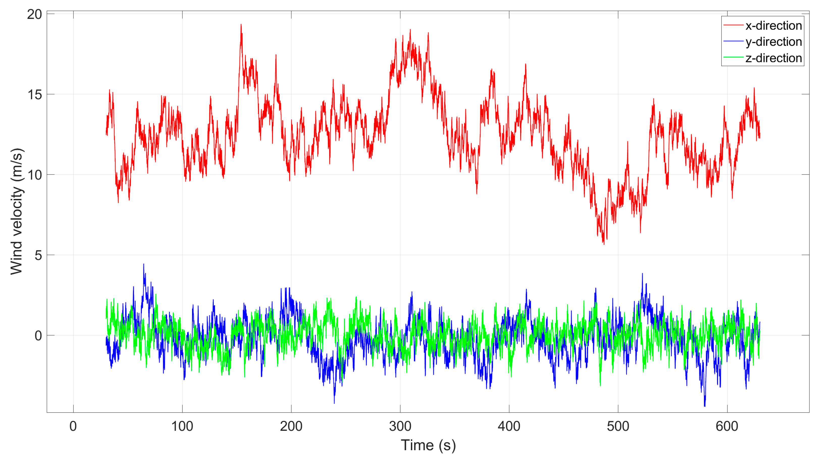
2.2. Wind Simulation

TurbSim [24], a wind turbulence simulator developed by NREL, generates 3D wind speed vector time series on a two-dimensional (2D) vertical grid. The program generates data based on a variety of meteorological conditions, including wind speed profiles, turbulence characteristics, and mean wind speed, and it converts frequency-domain velocity spectra to time-domain data by using the inverse Fourier transform. The generated wind field data are integrated with the AeroDyn [19] module of OpenFAST and used to analyze the dynamic loads acting on wind turbines. Taylor’s frozen turbulence hypothesis [25] is used to extend a 2D wind field to a 3D field, and the blade element momentum theory is used to compute the forces acting on turbine blades. Wind speed is expressed in terms of constant mean velocity and turbulence components, as shown in Equation (15).

$$V\left(\mathcal{z},t\right)=U\left(\mathcal{z}\right)+\upsilon (\mathcal{z},t)$$

(15)

where $V\left(\mathcal{z},t\right)$ is the wind speed measured at time $t$ at height $\mathcal{z}$ above the mean sea level (MSL) in a terrestrial or marine environment, $U\left(\mathcal{z}\right)$ is the mean wind speed at the aforementioned height, and $\upsilon (\mathcal{z},t)$ is the turbulent wind speed.

In this study, the power law [26] is used to represent the wind speed profile, as expressed in Equation (16).

$$\overline{V}\left(\mathcal{z}\right)={\overline{V}}_r{\left(\frac{\mathcal{z}}{{\mathcal{z}}_r}\right)}^{\alpha }$$

(16)

where ${\overline{V}}_r$ represents the wind speed at the hub height, and the power law exponent $\alpha$ depends on the surface roughness.

Wind turbulence refers to irregular fluctuations in airflow in the atmosphere. It significantly impacts the dynamic loads acting on wind turbines and the fatigue life of turbine materials. In this study, the Kaimal [27] turbulence model was used to generate a turbulent wind field according to the IA wind turbine class (IEC61400-1 classification [28]). The spectral density of wind speed is expressed by Equation (17).

$$S_U\left(f\right)={{\sigma }_U}^2\frac{4\frac{L_K}{U_{hub}}}{{(1+6\frac{f{L}_K}{U_{hub}})}^{(5/3)}}$$

(17)

where ${\sigma }_U$, $f$, and $L_K$ are the standard deviation of the wind speed, cycle frequency, and velocity component integration parameters, respectively.

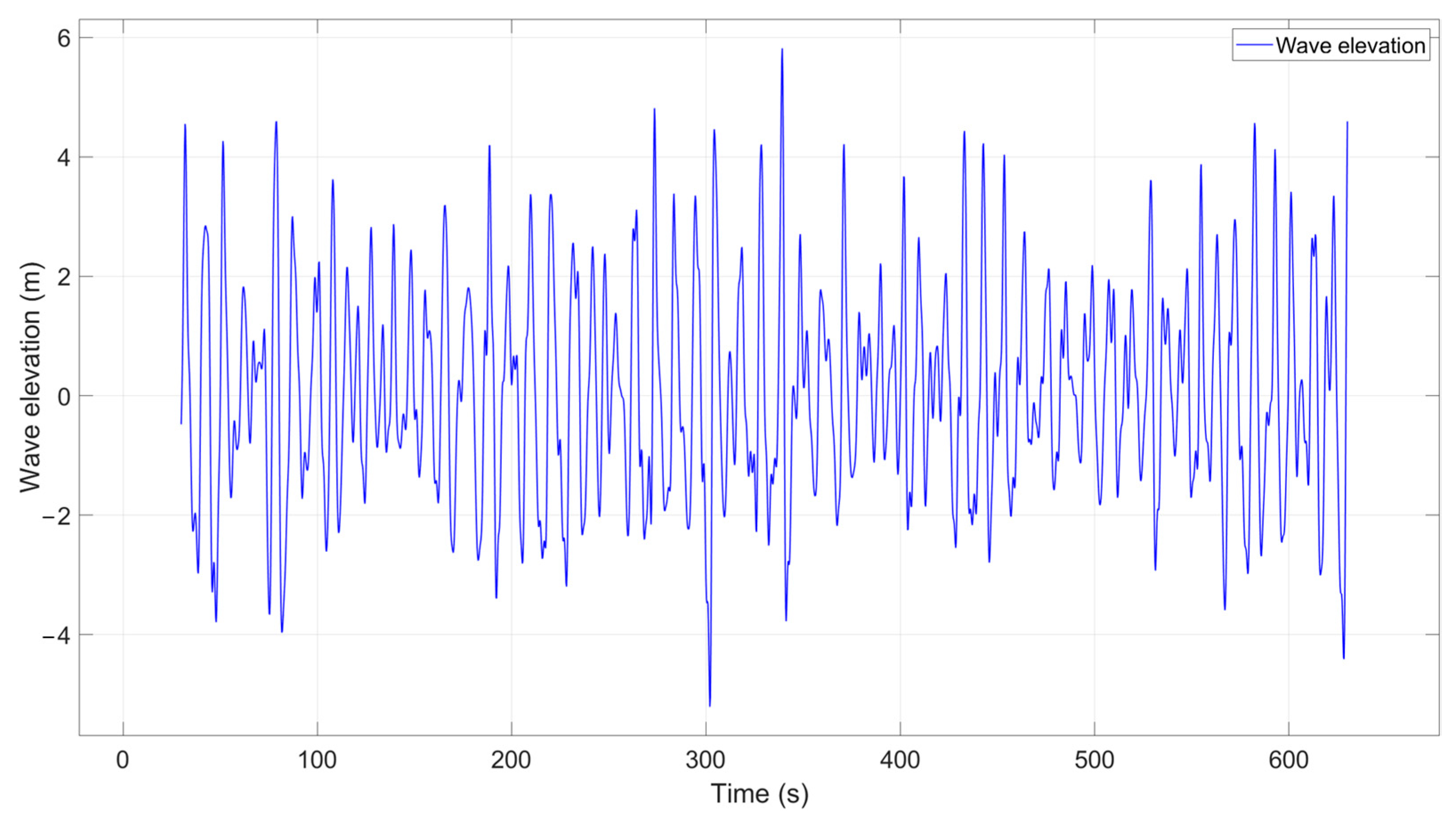
2.3. Wave Simulation

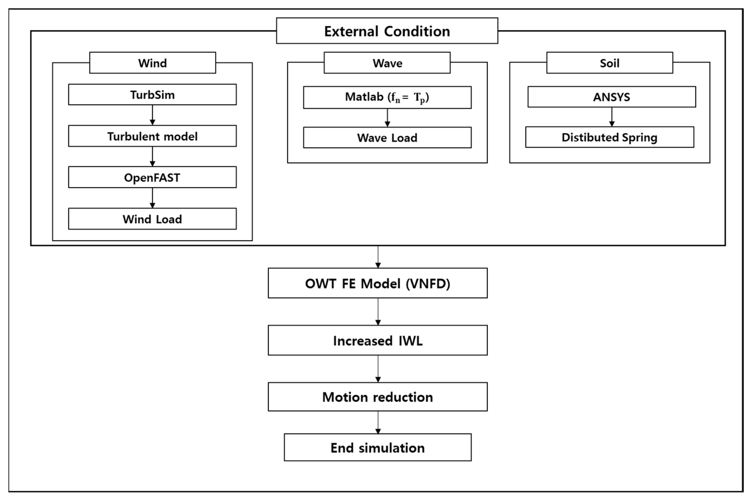
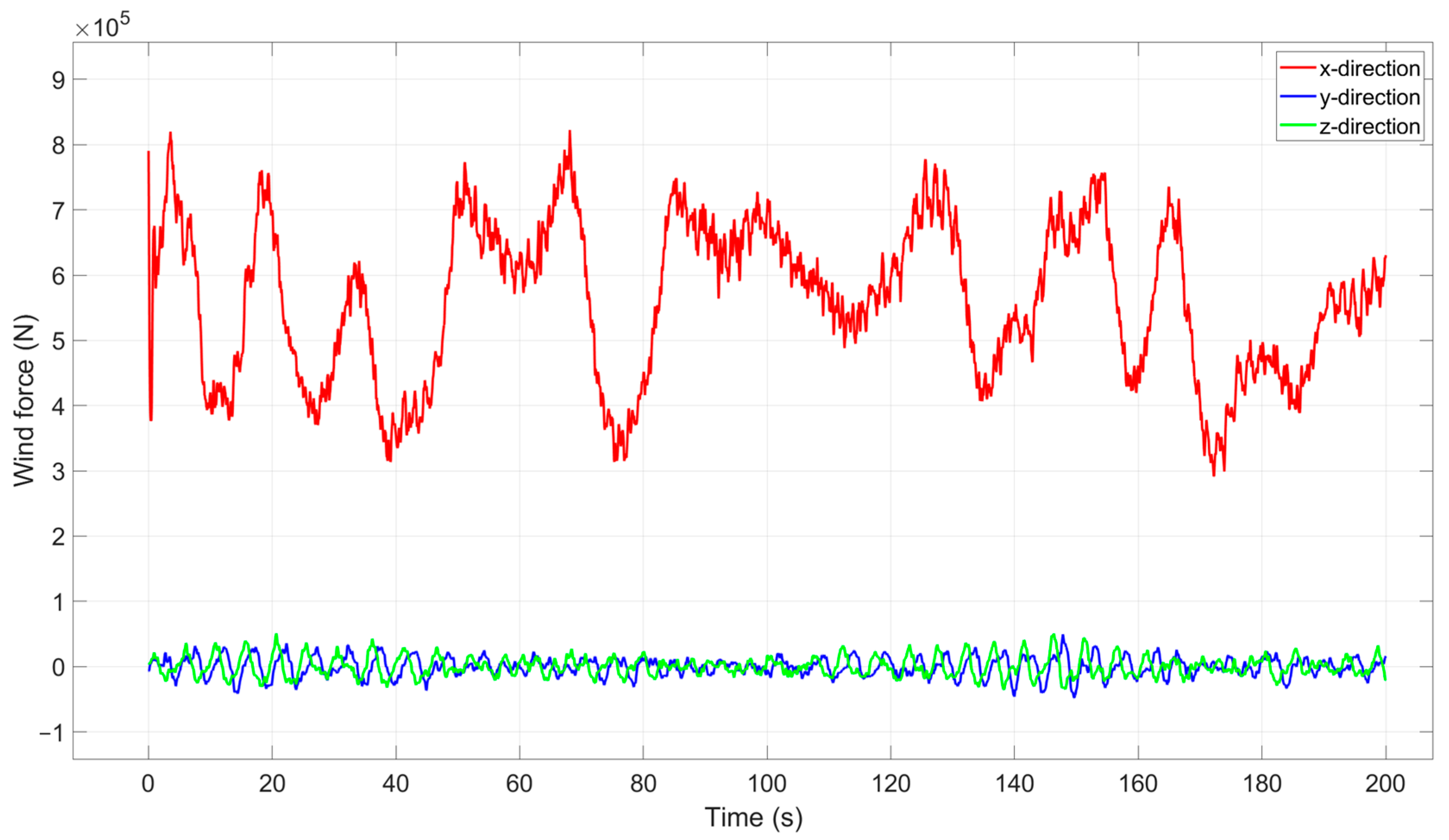
For irregular waves, the Pierson–Moskowitz [29] and JONSWAP spectra [30] are the most commonly used. The Pierson–Moskowitz spectral model describes the formation and development of ocean waves under certain wind conditions and predicts wave development and characteristics based on wind conditions. The JONSWAP spectral model, a modified version of the Pierson–Moskowitz spectral model that incorporates additional measurements related to the WAVE spectrum, was developed under the Joint North Sea Wave Project. This model is used to model developed sea states more accurately. According to DNV-OS-J101 [31], sea states at OWT sites should be modeled using the JONSWAP spectrum, unless there exist special circumstances or data. In this study, we used the JONSWAP spectral model in the validation phase, which is shown in Equation (18).

$$S\left(f\right)=0.3125H_S^2{T}_p{(\frac{f}{f_p})}^{5}exp[-\frac{5}{4}{\left(\frac{f}{f_p}\right)}^{-4}](1-0.287\mathrm{l}\mathrm{n}\gamma ){\gamma }^{exp[\frac{{\left(\omega -{\omega }_p\right)}^2}{2{\sigma }^2{\omega }_p^2}]}$$

(18)

where $T_p$ denotes the wave period, $H_S$ denotes the significant wave, and $f_p=\frac{1}{T_p}$, $\sigma$ is 0.07 for $f\le f_p$ and 0.09 for $f\ge f_p$. $\gamma$ is the JONSWAP peakedness parameter.

Wave loads acting on cylindrical slender structures, such as OWT monopiles, can be calculated using Morrison’s equation [32]. For an OWT monopile, the horizontal force A acting on a strip of length $z$ is given by Equation (19).

$$F_{wave}=F_M+F_D=C_M\rho \frac{\pi D^2}{4}{\int }_{-d_w}^{\eta \left(t\right)}\ddot{u}dz+C_D\rho \frac{D}{2}{\int }_{-d_w}^{\eta \left(t\right)}\dot{u}\left|\dot{u}\right|dz$$

(19)

where $F_M$ is the inertial force, $F_D$ is the drag force, $C_M$ is the mass coefficient, and $C_D$ is the drag coefficient. $D$ is the monopile diameter, and $\rho$ is the density of seawater, that is, 1025 $\mathrm{k}\mathrm{g}/{\mathrm{m}}^3$. $\dot{u}$ and $\ddot{u}$ denote the horizontal velocity and acceleration of water due to waves, $\eta \left(t\right)$ is the profile of the sea surface, and $d_w$ is the depth of water. Equations (20)–(22) are based on the linear wave theory of $\dot{u}$, $\ddot{u}$, and $\eta \left(t\right)$ [33].

$$\dot{u}=\frac{\pi h_{\omega }}{T_{\omega }}\frac{\mathit{sin}\left(k\right(\mathcal{z}+d_{\omega }\left)\right)}{\mathit{sinh}(k{d}_{\omega })}\mathit{cos}(kx-{\omega }_{\omega }t)$$

(20)

$$\ddot{u}=\frac{2{\pi }^2{h}_{\omega }}{{T_{\omega }}^2}\frac{\mathit{cos}\left(k\right(\mathcal{z}+d_{\omega }\left)\right)}{\mathit{sinh}(k{d}_{\omega })}\mathit{sin}(kx-{\omega }_{\omega }t)$$

(21)

$$\eta \left(t\right)=0.5h_{\omega }\mathit{cos}(kx-{\omega }_{\omega }t)$$

(22)

where $h_{\omega }, T_{\omega },$ $k$ and ${\omega }_{\omega }$ denote the wave height, wave period, number of waves, and wave frequency, respectively, and $\mathcal{z}$ is the vertical coordinate relative to the MSL.

3. Simulation

This study aims to effectively control the dynamic response of an OWT by using a VNFD. The research procedure is based on the flow diagram depicted in Figure 2. Given that a turbulent wind field was considered, a turbulence model was first generated using TurbSim, and then wind loads were calculated using OpenFAST v3.5.0. Meanwhile, wave loads in the form of sinusoidal waves with periods ($T_P)$ equal to the natural frequency ($f_n)$ of the structure were generated using MATLAB R2020a. Because this study was focused on evaluating the performance of the VNFD, forced resonances were generated by matching the wave period to the natural frequency of the structure to determine the effects of the IWL. These loads were applied to the ANSYS 2023 R1 coupled field transient, and the dynamic response of the structure was simulated by performing a one-way FSI analysis of the fluid and structure. In the one-way FSI, the interaction with the fluid outside the structure was assumed to occur as one-way pressure, which greatly improved the analysis efficiency [34]. Based on the simulation results, the resonance of the structure was investigated, and when resonance occurred, the water level inside the structure was adjusted to control the dynamic response of the structure due to resonance.

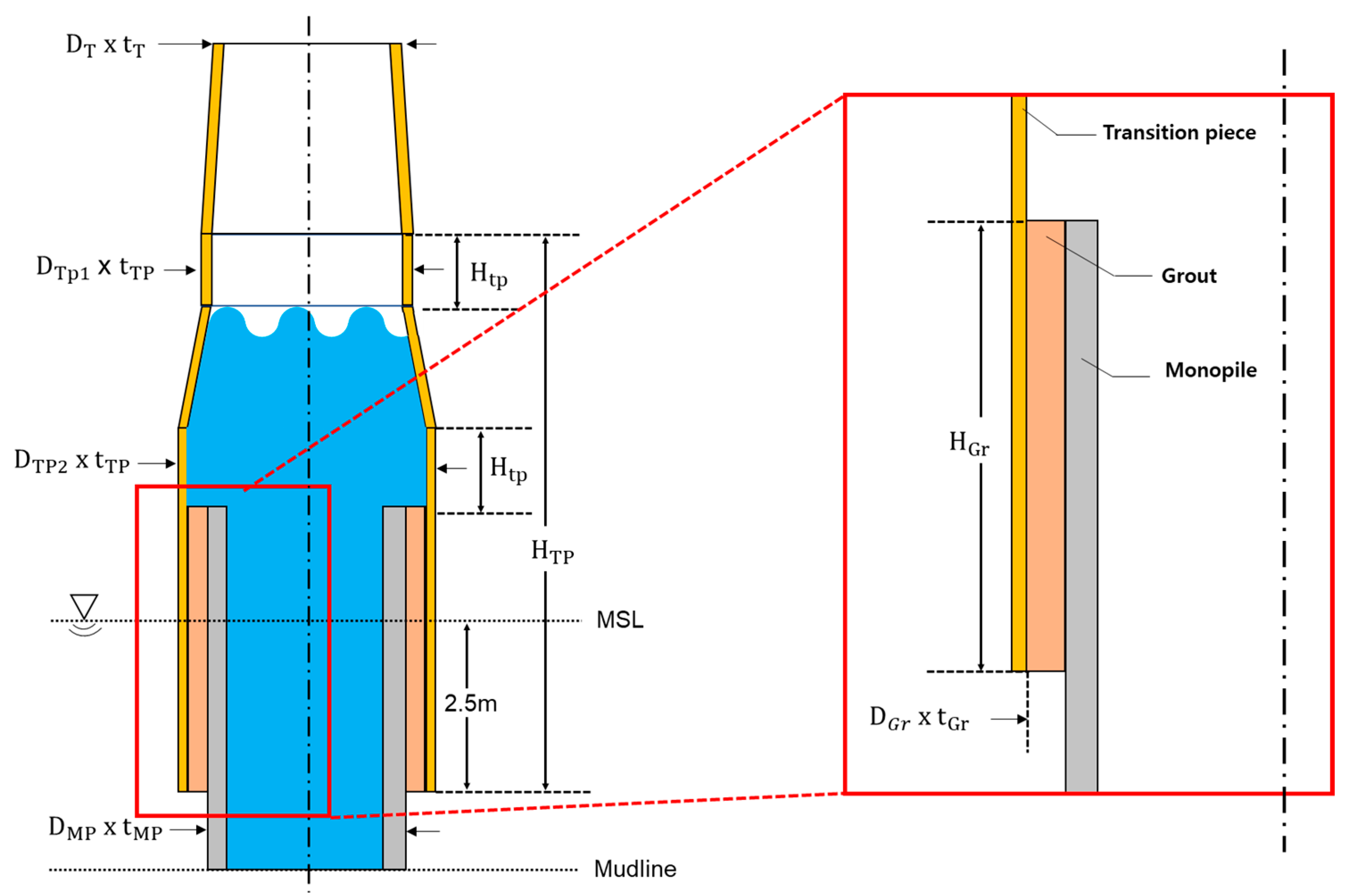
3.1. Wind Turbine Model Description

To study the dynamic response to environmental loads, the NREL 5 $\mathrm{M}\mathrm{W}$ turbine model was used in this study [35]. Figure 3 presents a schematic diagram of the reference wind turbine. The detailed specifications of the NREL 5 $\mathrm{M}\mathrm{W}$ turbine model are listed in

Table 1. Specification of NREL 5 $\mathrm{M}\mathrm{W}$ reference wind turbine [35].

Properties	$\mathbf{NREL}5\mathbf{M}\mathbf{W}$
Rated power ($\mathrm{M}\mathrm{W}$)	5
Rotor diameter ($\mathrm{m}$)	126
Rated wind speed ($\mathrm{m}/\mathrm{s}$)	11.4
Hub height ($\mathrm{m}$)	90
Total mass of tower ($\mathrm{t}\mathrm{o}\mathrm{n}$)	347.460
Outer diameter of tower top ($\mathrm{m}$)	3.87
Thickness of tower top ($\mathrm{m}$)	0.019
Outer diameter of tower bottom ($\mathrm{m}$)	6.0
Thickness of tower bottom ($\mathrm{m}$)	0.027
Tower height ($\mathrm{m}$)	87.6
Total weight of RNA ($\mathrm{t}\mathrm{o}\mathrm{n}$)	350
Pile thickness ($\mathrm{m}\mathrm{m}$)	60
Grout thickness ($\mathrm{m}\mathrm{m}$)	125
Grout diameter ($\mathrm{m}\mathrm{m}$)	6.25
Grout height ($\mathrm{m}$)	7.0
Transition piece thickness ($\mathrm{m}\mathrm{m}$)	30
Transition piece diameter ($\mathrm{m}$)	6.31
Transition piece height ($\mathrm{m}$)	12.5

, and the masses of the rotor and nacelle were set as separate lumped masses at the tower head, and this simplification method significantly reduced the computation time.

Table 2. Material properties of steel and grout.

Properties	Material
	Steel [36]	Grout [14]
Young’s modulus, $E$ ($\mathrm{G}\mathrm{P}\mathrm{a}$)	210	70
$\mathrm{Density}, \rho$$(\mathrm{k}\mathrm{g}/{\mathrm{m}}^3$)	8500	2740
Poisson’$\mathrm{s} \mathrm{ratio}, \upsilon$ (-)	0.38	0.19

lists the properties of the constituent steel, and the tower material density was set to 8500 $\mathrm{k}\mathrm{g}/{\mathrm{m}}^3$ to account for the bolts, paint, welds, and flanges [15,36,37]. The material of the support structure was specified as S355, which is commonly used in OWTs, and Ducorit D4 [14] was used as the grout. The soil material properties were modeled as constant, with depth with a Poisson’s ratio of 0.3, cohesion of 0.05 $\mathrm{K}\mathrm{P}\mathrm{a}$, and effective unit weight of 10 $\mathrm{K}\mathrm{N}/{\mathrm{m}}^3$, referring to the geotechnical model of OC3 [38]. For other depth-dependent soil material properties, see Figure 3. The soil deposit was assumed to be composed of a sandy layer with no clay, and the fluid was assumed to be seawater with a density of 1025 $\mathrm{k}\mathrm{g}/{\mathrm{m}}^3$ [39].

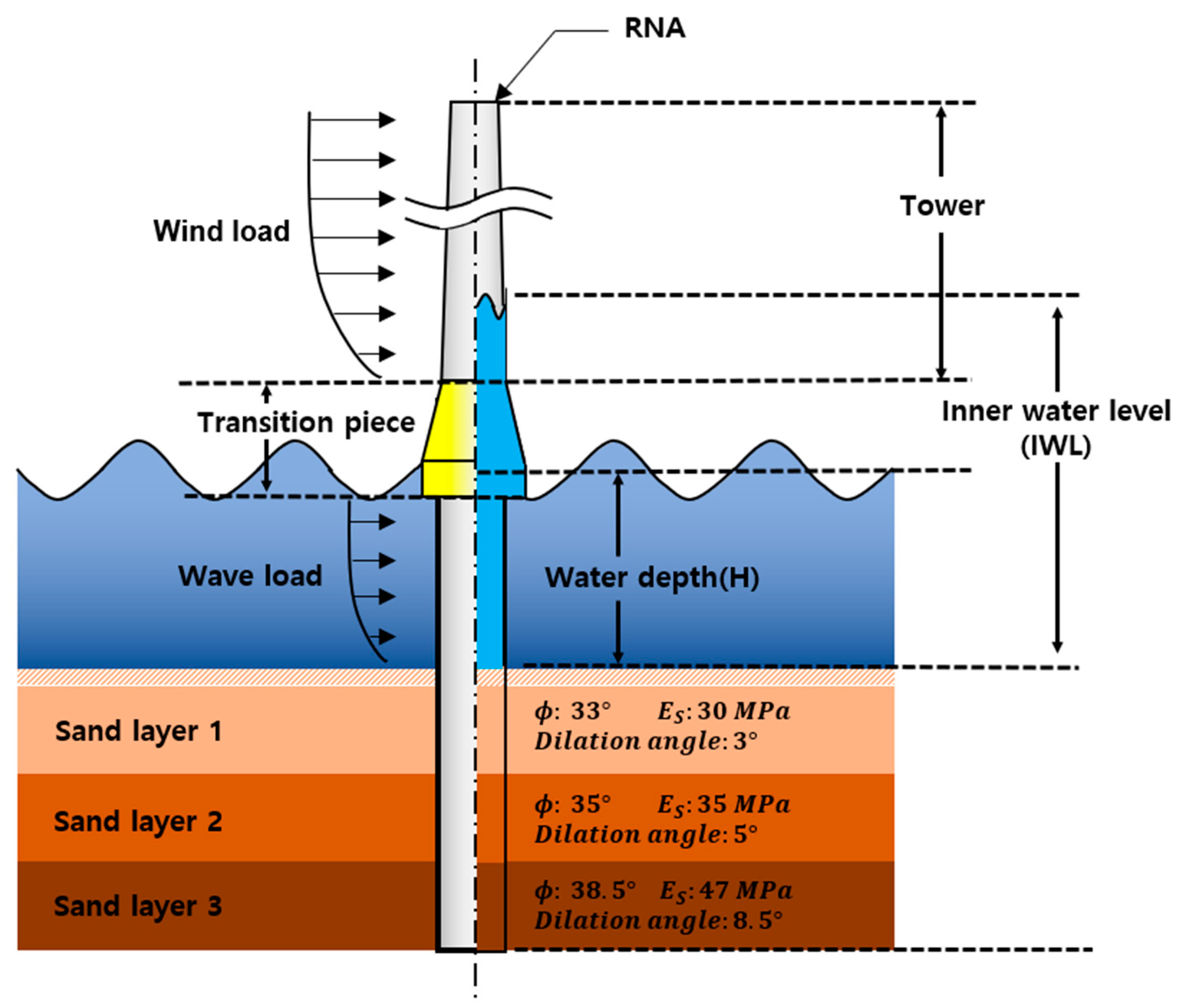
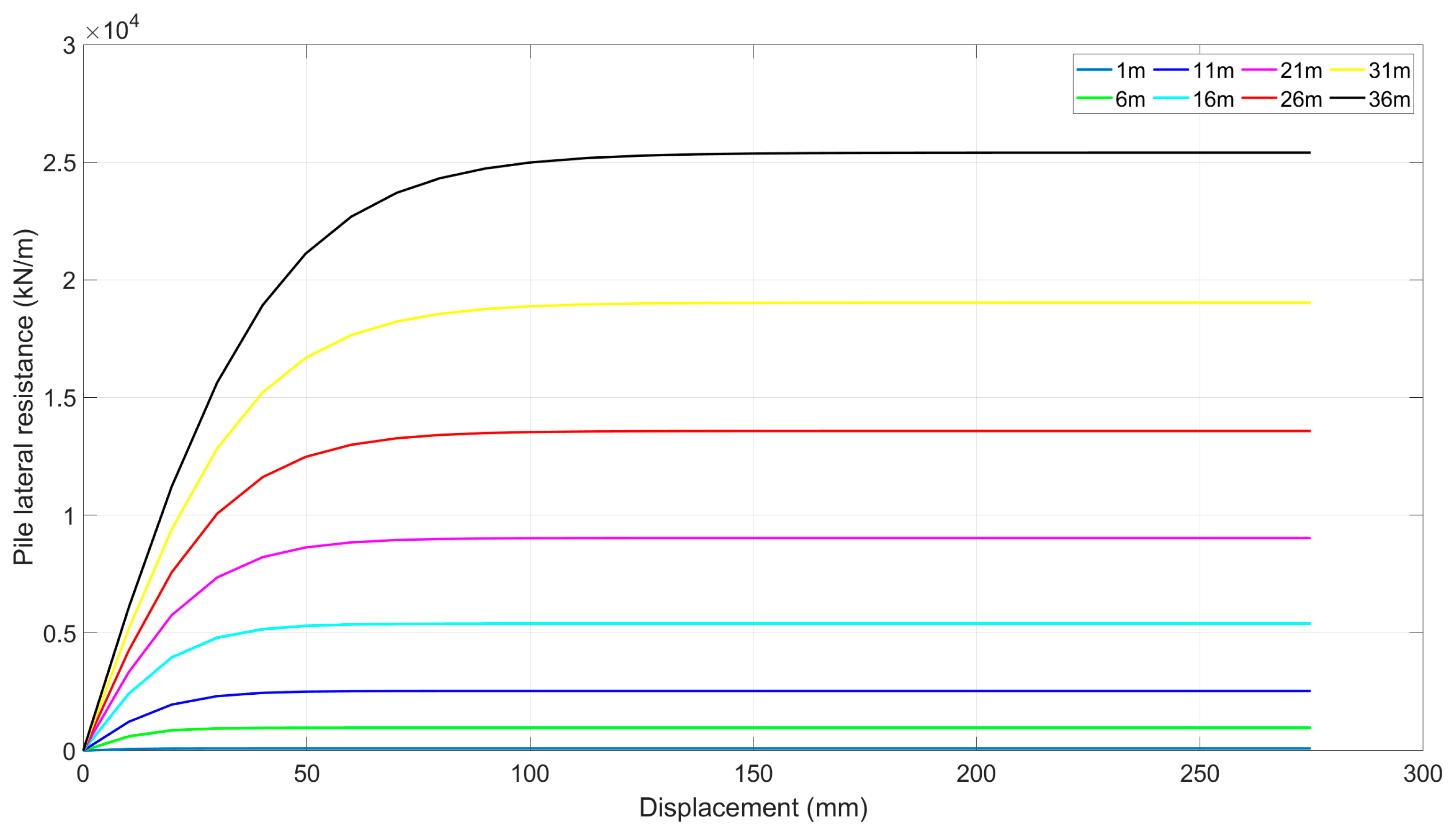
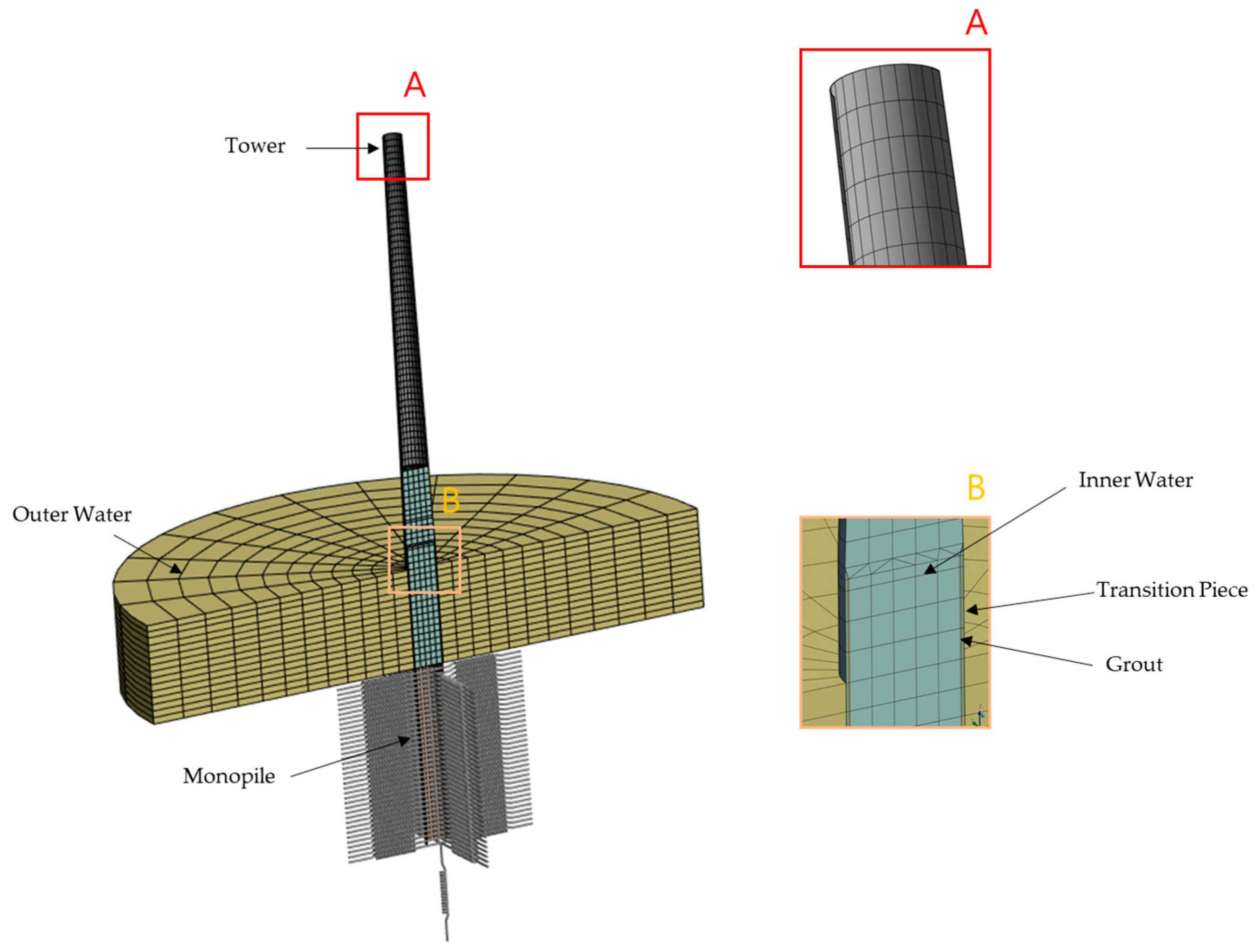
3.2. Setting Up the Analysis Model

The objective of this dynamic study was to minimize the amplitude due to resonance by using a VNFD. Dynamic analysis without considering SSI may yield inappropriate results. According to DNVGL-ST-0126 [3], a design standard for wind turbine support structures, appropriate stiffness values should be applied to the ground support foundation in dynamic analyses of wind turbine structures. Soil stiffness can be modeled using methods such as apparent fixity (AF), coupled spring (CS), and distributed spring (DS). Each method can describe the behavior of monopiles through linear or nonlinear stiffness in both lateral and vertical directions. For a detailed explanation of each method, please refer to the study by Zaaijer M.B. [40]. In general, the main method used to consider the SSI is the p-y [41] or 3D FEA method. The p-y method simplifies the transverse SSI by using nonlinear springs to connect the horizontal resistance $p$ and the corresponding displacement $y$ when modeling the SSI. Among the p-y methods, the distributed spring (DS) method is widely used in OWT-related studies because it offers a good balance between analysis accuracy and computational cost [42]. Therefore, the DS method was used to economize the analysis process. The DS method was applied through the nonlinear spring element (COMBIN39) [43] for both lateral and vertical directions, as illustrated in Figure 4. COMBIN39 is capable of describing the nonlinear relationship between compression and tension stiffness (force–displacement) for transversal or torsional directions. Torsional stiffness for lateral and vertical springs was not considered, and lateral springs were modeled at 1 m intervals to describe the soil depth profile while constraining the torsional degrees of freedom (DOF) of COMBIN39; rotation in the torsional direction of the monopile was not allowed as an additional constraint. To minimize the change in stiffness direction of COMBIN39 in the x-direction due to displacement in the y-direction of the monopile, the physical distance of COMBIN39 was set to a sufficient margin of 20 $\mathrm{m}$. DS stiffness values were derived, as shown in Figure 5, through properties of the sand layer described above and arbitrary monopile head displacement using PileLAT 2.3 software. For visibility, Figure 5 is represented at intervals of 5 $\mathrm{m}$ from 1 $\mathrm{m}$ to 36 $\mathrm{m}$. The p-y model used in PileLAT is as per Equation (23).

$$\begin{array}{c}{P}_{us}=\left(C_{1}X+C_{2}D\right){\gamma }^{\prime }X\\ P_{ud}=C_{3}D{\gamma }^{\prime }X\end{array}$$

(23)

where $P_{us}$ represents the ultimate resistance at a shallow depth, $P_{ud}$ denotes the ultimate resistance at a deep depth, ${\gamma }^{\prime }$ is the effective soil weight, $X$ signifies depth, $C_1, C_2, {\mathrm{a}\mathrm{n}\mathrm{d} C}_3$ are coefficients determined from Figure A.6-2 of API RP 2GEO [44], and $D$ is the diameter of the pile.

The tower, grout, TP, monopile, and water were modeled as 3D SOLID elements. The structure was modeled as a 20-node 3D structural elements (Solid 186), and the internal and external fluids were modeled as 20-node 3D acoustic fluid elements (Fluid 220) to determine their acoustic properties. Gravitational acceleration along the z-direction was set to 9.81 $\mathrm{m}/{\mathrm{s}}^2$. Moreover, it was assumed that water only transmitted pressure, and there was no gap or transverse friction. The RNA located at the top of the tower originally had a complex structure and mass distribution, but by applying simplifying assumptions, the mass of each rotor and nacelle was represented as a point mass. Figure 4 shows the developed FE model.

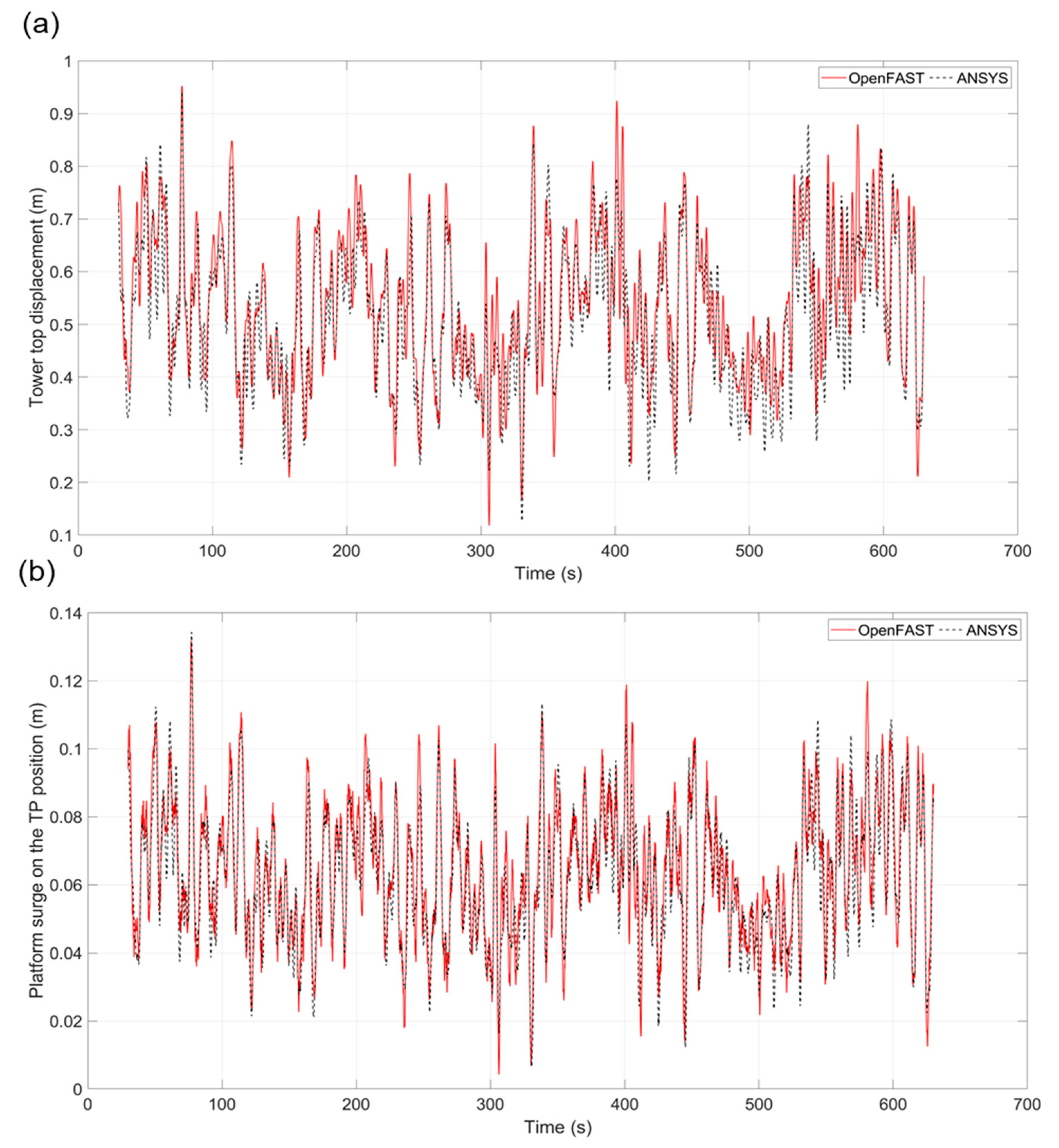
3.3. Verification of FE Model

To ensure the reliability of the developed FE model, mesh convergence was first performed [12]. In this process, convergence of the natural frequency was examined by gradually increasing the number of mesh divisions along the circumferential and vertical directions of the structure. The number of divisions at the radial edges of the outer water, which were not included in the verification stage but were used in this study, allowed for the use of the bias factor to create a finer mesh in the contact area between the monopile and water. The results are listed in

Table 3. Results of mesh convergence test.

Number of Elements	Natural Frequency ($\mathbf{H}\mathbf{z}$)	Diff (%)
8472	0.2488	0
9144	0.24885	0.02
11,076	0.24889	0.02
14,768	0.2491	0.08
22,152	0.2492	0.04
37,824	0.24918	−0.01
45,116	0.24924	0.02

.

As listed in Table 3, the error rate in natural frequency was the least when the number of elements increased from 22,152 to 37,824, and therefore, this value was considered the most appropriate in this study. The number of divisions on the circumferential edge of the structure were set to 24 and those on the radial edge of water were set to 12 divisions. The longitudinal edge was divided into 1.5 m long segments.

To verify the analytical model, only the first-order natural frequencies of the NREL 5 MW OC3 model with a rigid base and flexible foundation were compared to those obtained in other works [22,38], because VNFD mainly deal with the soft–soft and soft–stiff domains. The first-order fore-aft and side-to-side natural frequencies of the wind turbine were calculated and compared with those obtained in other studies.

As a result, we found a maximum deviation of 3.95$\mathrm{\%}$ in the flexible foundation fore–aft, as listed in

Table 4. Comparison of the simulation results of the FE model with the results of other studies of the NREL turbine model for the rigid base (RB), flexible foundation (FF) condition.

Model	Natural Frequency ($\mathbf{H}\mathbf{z}$)		Relative Difference (%)
	1st Fore–Aft	1st Side-to-Side	1st Fore–Aft	1st Side-to-Side
Rigid base (present)	0.3242	0.3247	-	-
Rigid base [22]	0.3132	0.3132	3.39	3.54
Flexible foundation (present)	0.2509	0.2512	-	-
Flexible foundation [38]	0.2410	0.2420	3.95	3.65

, which confirmed the validity of the proposed model.

To further validate the model, the results of the time response of the top displacement of the tower and the platform surge at the TP were compared between ANSYS and OpenFAST. For this purpose, wind and wave loads were generated and applied in the analysis. The size of the generated wind field was 145 $\mathrm{m}$ × 145 $\mathrm{m}$. The wind field centered on the hub was discretized with a finite grid in both the horizontal and vertical directions. Based on DLC 1.2, the wind field was modeled using the normal turbulence model (NTM), and the mean wind speed was modeled as 12 $\mathrm{m}/\mathrm{s}$, similar to the rated wind speed. A power law index of 0.14 was used. The water depth, wave height, and wave period were set to 20 $\mathrm{m}$, 8.24 $\mathrm{m}$, and 10 $\mathrm{s}$, respectively. The wind and wave data were segmented into 0.05 $\mathrm{s}$ intervals over a duration of 600 $\mathrm{s}$, excluding the initial 30 $\mathrm{s}$, as illustrated in Figure 6 and Figure 7.

A Rayleigh damping model was considered throughout the analysis, and a damping ratio of 5$\mathrm{\%}$ was used to account for aerodynamic and hydrodynamic damping effects [45]. To set the boundary conditions, the obtained wind load was applied to the RNA at the top of the tower, and wave load was applied to the TP portion near the MSL.

Figure 8 presents a comparison of the time response of the top displacement of the fore–aft tower and the platform surge in the TP section. The maximum displacement, average displacement, and standard deviation of the time response were compared and analyzed, as summarized in

Table 5. Comparison of displacement results obtained using OpenFAST and ANSYS.

	Tower Top Displacement ($\mathbf{m}$)			Platform Surge on TP ($\mathbf{m}$)
	OpenFAST	ANSYS	Diff ($\mathbf{m}$)	OpenFAST	ANSYS	Diff (%)
Max	0.952	0.941	1.15	0.132	0.134	−1.91
Mean	0.537	0.512	4.65	0.064	0.062	2.96
Std	0.139	0.134	3.42	0.020	0.019	3.29

. Although there were slight differences between the two sets of data, the overall trend was consistent, thereby validating the dynamic response analysis.

The error rate in the results was attributed to inconsistencies in the dynamic properties of the numerical model of the OWT structure. OpenFAST included and calculated the dynamic effects of blade rotation by using the AeroDyn module, while ANSYS modeling did not fully reflect the dynamic behavior of such rotation. In addition, the wind and wave loads calculated using the AeroDyn and HydroDyn modules were distributed over multiple nodes of the turbine in OpenFAST, resulting in the full dynamic behavior of the system. By contrast, in the ANSYS model, the wind load was concentrated near the top RNA of the tower, and the wave load was concentrated in the TP near the MSL, resulting in a simplified load distribution. Moreover, there were differences in soil modeling: for the same physical properties, OpenFAST used a coupled spring (CS) soil model to model the effects of the SSI, while ANSYS used a distributed spring (DS) soil model. The aforementioned slight deviations could be attributed to these differences.

4. Results and Discussions

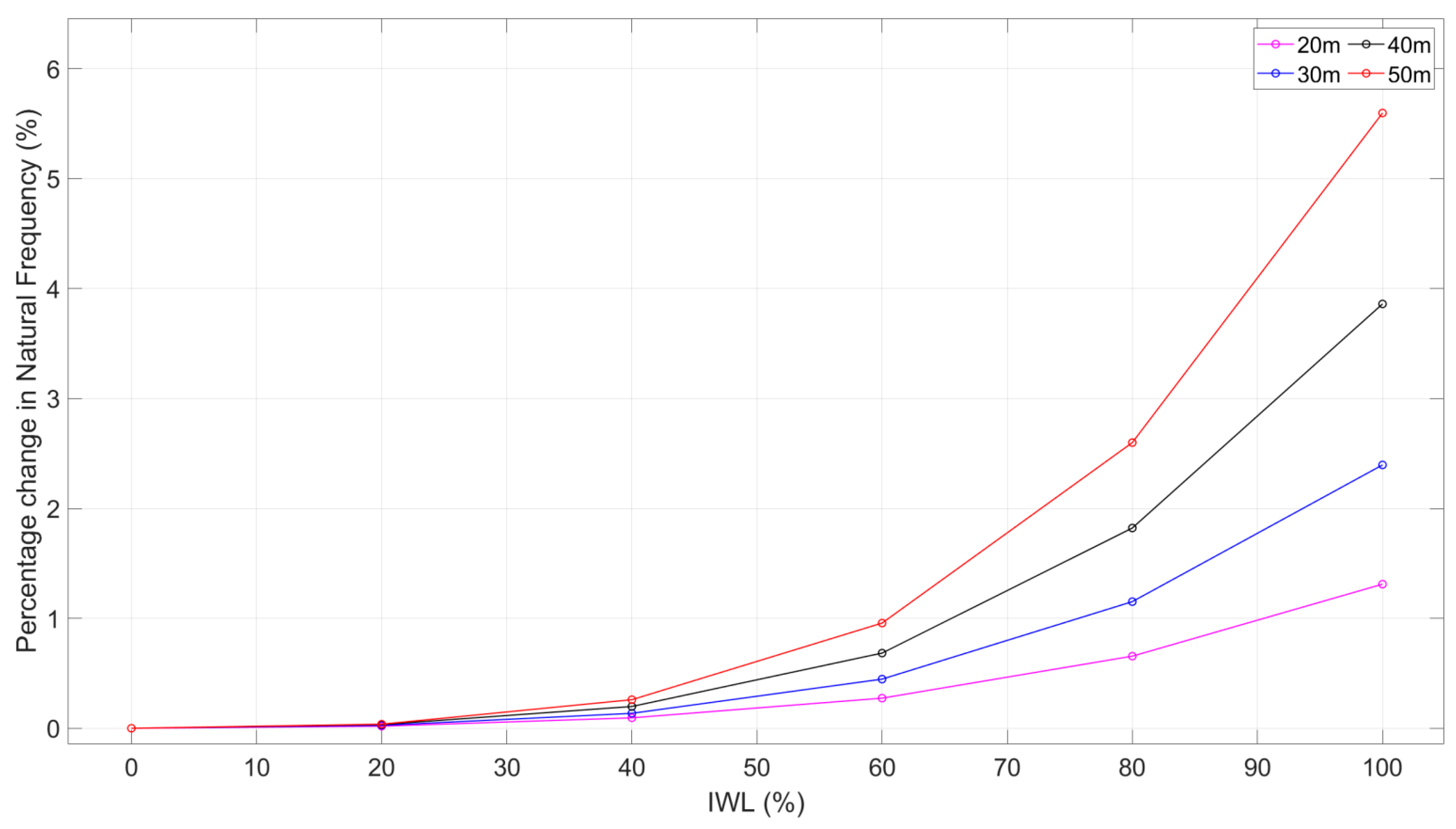
4.1. Changes in Natural Frequency with Inner Water Level

Natural frequency variations resulting from VNFD use should be studied to understand the amplitude response of OWTs due to resonance. In this chapter, the effect of IWL on natural frequency is studied to provide basic data for dynamic control effects, such as amplitude reduction.

The results obtained using the natural frequency calculation formula derived in this study were compared to the simulation results obtained by using ANSYS to validate the formula. Equation (24) was obtained by substituting Equations (10) and (11) into Equation (12).

$$f_{RB(tapered+SS+w)}=\frac{1}{2\pi }\sqrt{\frac{k_{T(tapered+SS)}}{m_{RNA}+\alpha m_{T(tapered+SS)}+\frac{\psi \left(m_{mono}+m_{TP}+m_{tower}\right)\xi ({CG}_W+H)}{m_{RNA}({CG}_{RNA}+H)}}}$$

(24)

where $\xi$ is the ratio of the water level inside the structure, and $\psi$ was calibrated to 0.0164 under the inner fluid simplification assumption. As can be inferred from

Table 6. Comparison of natural frequency estimates for flexible foundation with consideration of water and simulation result.

Water Depth ($\mathbf{m}$)	${\mathit{f}}_{\mathit{R}\mathit{B}(\mathit{t}\mathit{a}\mathit{p}\mathit{e}\mathit{r}\mathit{e}\mathit{d}+\mathit{S}\mathit{S}+\mathit{w})}$ ($\mathbf{H}\mathbf{z}$)	Simulation Result ($\mathbf{H}\mathbf{z}$)	Difference (%)
20	0.2662	0.2517	5.46
30	0.2447	0.2283	6.69
40	0.2241	0.2075	7.42
50	0.2048	0.1882	8.09

, the error rate between the theoretically calculated natural frequency values and the simulation results was not significant at low water depths, but it increased consistently as the water depth increased. This suggests that the model may yield larger errors when predicting the system behavior at greater depths.

The scenarios were set at 20$\mathrm{\%}$ increments from 0 to 100$\mathrm{\%}$ depending on the IWL. The results are listed in

Table 7. Results of natural frequency analysis for first fore–aft mode.

IWL (%)	Water Depth ($\mathbf{m}$)
	20	30	40	50
0	0.2517	0.2283	0.2075	0.1882
20	0.2516	0.2282	0.2074	0.1881
40	0.2514	0.2280	0.2071	0.1877
60	0.2510	0.2273	0.2061	0.1864
80	0.2500	0.2257	0.2037	0.1833
100	0.2484	0.2228	0.1995	0.1776

, and according to them, as the IWL increases, the amount of water increases, and the resulting increase in mass lowers the natural frequency of the system.

Table 8. Percentage of change in natural frequency with inner water level and water depth.

IWL (%)	Water Depth ($\mathbf{m}$)
	20	30	40	50
0	-	-	-	-
20	0.019	0.026	0.034	0.037
40	0.095	0.136	0.198	0.260
60	0.274	0.447	0.684	0.957
80	0.656	1.152	1.822	2.599
100	1.311	2.396	3.860	5.596

summarizes the variation in natural frequency with depth as a function of the IWL. At 20 $\mathrm{m}$, the controllable natural frequency range is 1.311$\mathrm{\%}$, while at 50 $\mathrm{m}$, it is 5.596$\mathrm{\%}$, thus confirming that the controllable natural frequency range increases with depth, as illustrated in Figure 9.

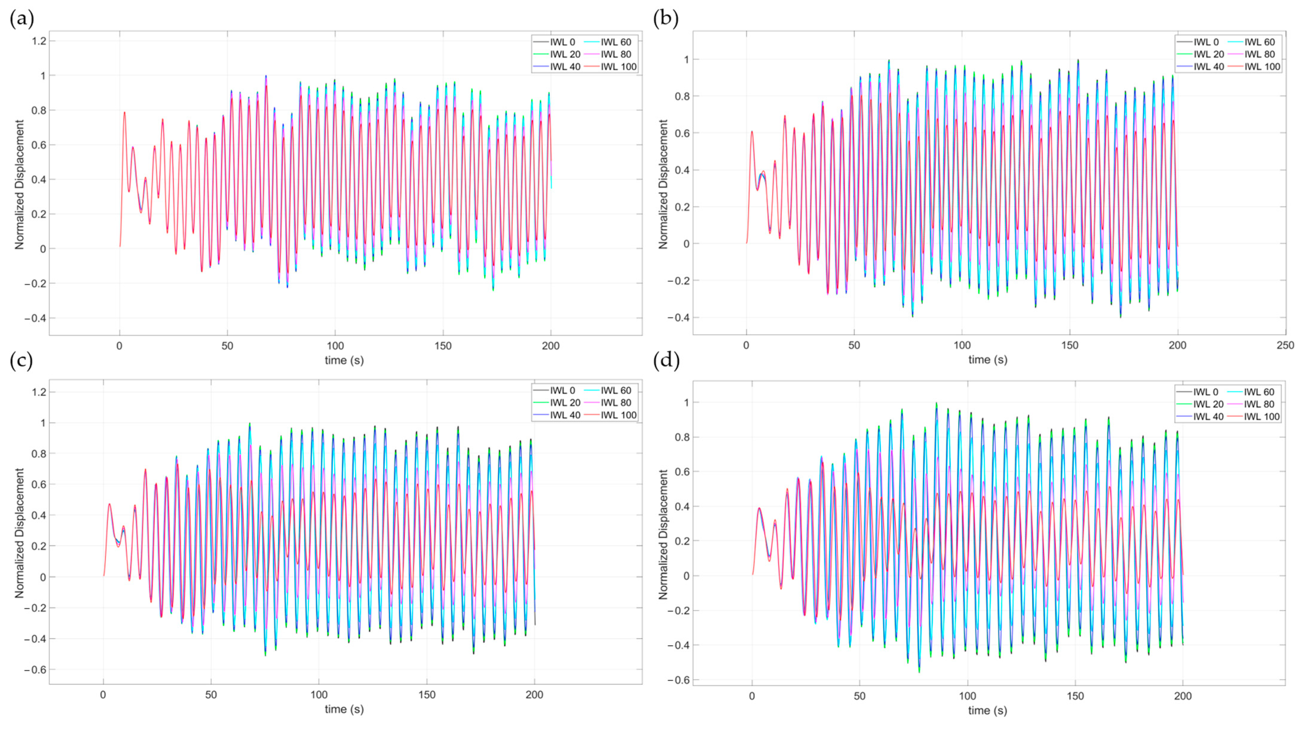
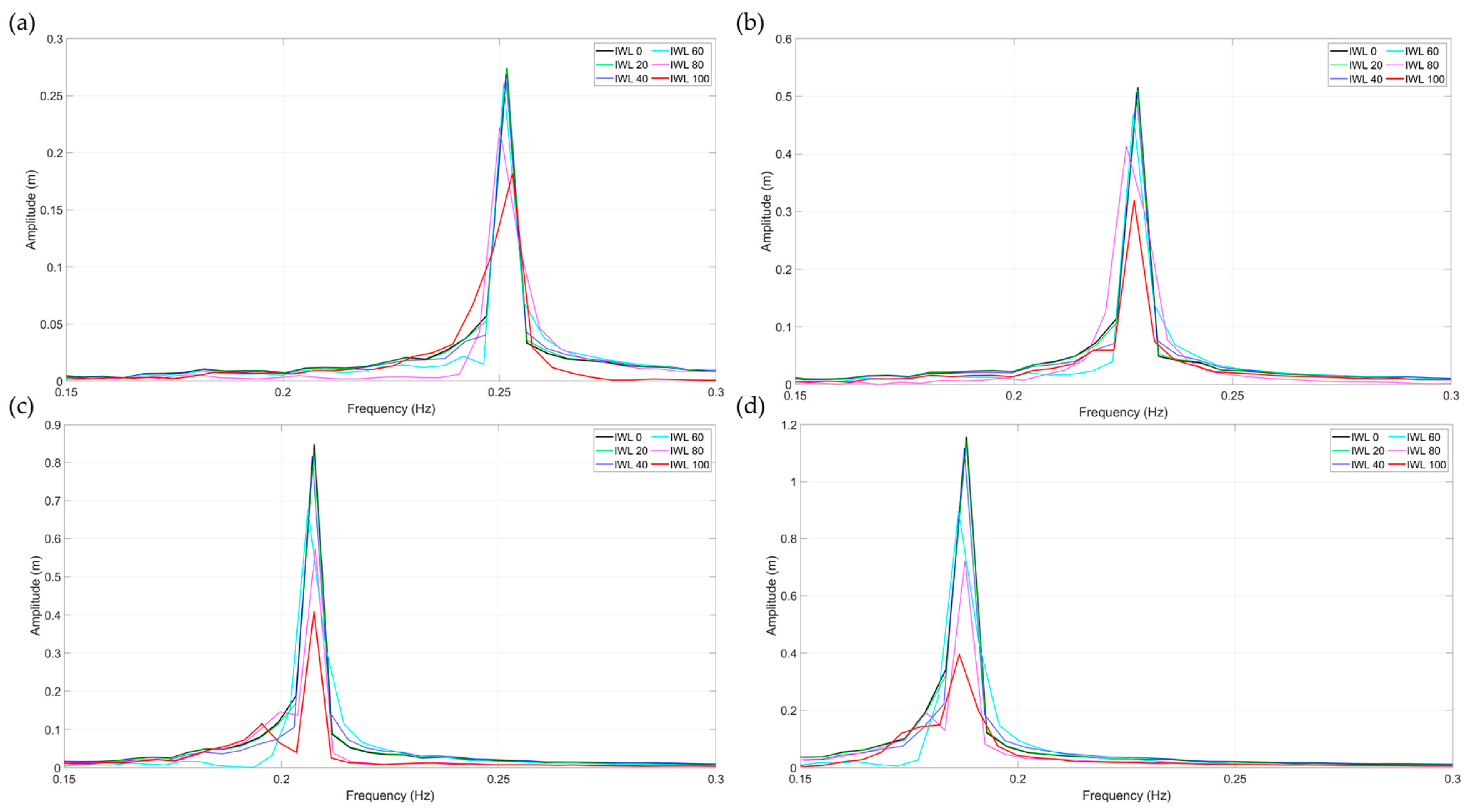
4.2. Reducing Dynamic Response to Changes in Natural Frequency

In the previous section, the change in natural frequency with the IWL was studied by using a VNFD. An increase in the IWL leads to a decrease in the natural frequency, thus suggesting that the vibration response of the structure can be reduced for loads that have the same period as the natural frequency. In particular, the change in natural frequency is greater at a depth of 50 $\mathrm{m}$ than that at a depth of 20 $\mathrm{m}$, and the amplitude reduction is expected to be greater with increasing water depth. Therefore, in this section, the effect of natural frequency reduction on the amplitude reduction in OWTs in different depth IWL scenarios is analyzed.

The main objective of this study is to analyze the performance of the VNFD in terms of improving the structural stability of OWTs. For this purpose, a wave load in the form of a sinusoidal wave with a period corresponding to the natural frequency of the structure in the absence of seawater inside the structure is applied to induce a forced resonance phenomenon. Then, the effect of amplitude reduction resulting from the IWL adjustment is analyzed.

The wave loads were generated using MATLAB based on Morrison’s equation, and assumed to have a wave period consistent with the natural frequency of the structure in terms of depth, as summarized in

Table 9. Wave periods based on natural frequency of structure.

Water Depth ($\mathbf{m}$)	Natural Frequency ($\mathbf{H}\mathbf{z}$)	Wave Period ($\mathbf{s}$)
20	0.2517	3.97
30	0.2283	4.38
40	0.2075	4.82
50	0.1881	5.31

, and a wave height of 1.3 $\mathrm{m}$. It is a regular sine wave in the form of sin ($\mathsf{\omega }\mathrm{t}+\mathrm{b}$). The density of water was set to 1025 $\mathrm{k}\mathrm{g}/{\mathrm{m}}^3$, and the inertia and drag coefficients were assumed to be 1.2 and 1.0, respectively [46]. According to a study of the NREL 5 $\mathrm{M}\mathrm{W}$ reference turbine, wind loads have a greater effect on the dynamic behavior of the structure than wave loads [47]. Therefore, wind loads were included in the load data to represent more accurately the behavior of the OWT in real-world environments. These wind loads were generated using a turbulence model created with TurbSim, and the same modeling parameters and values were used in the validation phase. The resulting turbulence conditions were then represented as wind loads by using OpenFAST software. The wind loads used in this study are depicted in Figure 10. The generated wind and wave loads were applied to the TP sections near the RNA and MSL, respectively.

Figure 11 depicts the response of the tower top fore–aft of the OWT. With no seawater in the structure, the structure experienced the maximum resonance when the wave period matched its natural frequency, resulting in the largest displacement at the top of the tower. As the water level increased, as shown in the graph, there was a gradual decrease in the top displacement of the tower. For water depths of 20, 30, 40, and 50 $\mathrm{m}$, the peak displacement of the top of the tower decreases with the IWL by up to 5.8$\mathrm{\%}$, 18.1$\mathrm{\%}$, 26.7$\mathrm{\%}$, and 34.5$\mathrm{\%}$, respectively.

According to Figure 11, the dynamic response to IWL changes was weaker in the early stages. This could probably be attributed to the direct influence of the external loads that the structure was subjected to initially, and as a result, IWL changes did not cause immediate changes in the dynamic response of the tower. However, as the structure stabilized over time, the vibration response of the structure was dominated by changes in its natural frequency. As a result, the change in natural frequency due to the increase in the IWL appeared to significantly influence the dynamic response of the structure.

In addition, Figure 12 shows the frequency spectra obtained by Fast Fourier Transform (FFT) of the tower top displacement response, and according to the analysis, the tower top peak displacement decreased by up to 33$\mathrm{\%}$, 37$\mathrm{\%}$, 51$\mathrm{\%}$, and 65$\mathrm{\%}$, respectively, as the IWL changed with water depth.

According to the results, the variation in the tower top displacement in the time response was relatively small. This may be because of the fact that the damping characteristics were not analyzed directly in this study. Although damping is an important factor affecting vibration energy dissipation in a structure, this study focused on analyzing the dynamic response of the structure at a fixed IWL value. Therefore, the change in the time response could not be attributed directly to the energy dissipation caused by damping, and it was presumed to be related to the change in the natural frequency. Meanwhile, in the frequency response analysis, when the frequency of the wave load matched the natural frequency of the structure, the energy was concentrated owing to the resonance phenomenon, which appeared as a high-energy-density peak in the FFT analysis. This resonance phenomenon affected the response of the structure, and changing the natural frequency by adjusting the IWL reduced the heights of these energy density peaks. This change dramatically diminished the displacement peak in the frequency response.

Table 10. Rate of change in sequential maximum displacement response with increasing IWL and depth in frequency domain.

IWL (%)	Depth ($\mathbf{m}$)
	20	30	40	50
0	-	-	-	-
20	−0.007	0.648	1.295	0.721
40	1.598	1.028	2.404	2.512
60	3.065	7.073	17.041	19.801
80	14.962	12.101	15.245	19.341
100	18.098	22.711	28.743	45.276

shows the rate of change in displacement with the IWL and depth in the frequency spectrum. The difference between the displacement due to IWL changes at the minimum altitude, where the IWL increases from 0 to 20$\mathrm{\%}$ at a depth of 20 $\mathrm{m}$, and the displacement due to IWL changes at the maximum altitude, where the IWL increases from 80 to 100$\mathrm{\%}$ at a depth of 50 $\mathrm{m}$, was significant. In particular, at a depth of 50 $\mathrm{m}$, the amplitude reduction effect of the minimum height was extremely small, at 0.72$\mathrm{\%}$, while the amplitude reduction effect of the maximum height was 45.3$\mathrm{\%}$, which is 62.9 times greater.

$${\alpha }_w=\psi \frac{m_w(C{G}_w+H)}{m_{RNA}(C{G}_{RNA}+H)}$$

This is expressed in Equation (11). The increase in the IWL caused the center of gravity of the water inside the structure, $C{G}_w$, to rise, and consequently, the equivalent mass ratio, ${\alpha }_w$, also increased. This caused $m_w$ to contribute to the vibration of the structure at higher positions, making the reduction in natural frequency greater. The rise in the center of gravity was especially significant when the water depth increased and the IWL was significantly higher simultaneously; in this condition, the vibration amplitude decreased significantly.

5. Conclusions

In this work, the VNFD of a monopile-type OWT was studied, where the IWL was adjusted to alter the natural frequency of the structure to achieve an amplitude reduction effect. In the course of the study, changes in natural frequency were analyzed in various IWL scenarios at different water depths, and the effects of these changes on the dynamic behavior of the OWT due to resonance, especially amplitude, were studied.

The analysis showed that the increase in the IWL was directly related to the increase in system mass, which led to a decrease in its natural frequency and a shift away from the resonant frequency. The time response of the tower top fore–aft peak displacement of the OWT exhibited the maximum effect of 5.8$\mathrm{\%}$ at a depth of 20 $\mathrm{m}$ and a relatively large reduction of 34.5$\mathrm{\%}$ at a depth of 50 $\mathrm{m}$. The frequency spectrum obtained by FFT showed a reduction of 33$\mathrm{\%}$ at a depth of 20 $\mathrm{m}$ and 65$\mathrm{\%}$ at a depth of 50 $\mathrm{m}$. These results were obtained by focusing on reducing energy density, which entailed changing the natural frequency. By combining the VNFD with a damper system that dissipates vibration energy, a stronger effect can be expected in terms of reducing the amplitude and improving the stability of the structure.

In addition, the increase in the IWL caused the center of gravity of the water to rise, and as a result, the mass of water contributed to the vibration of the structure at a higher position, resulting in greater reduction in the natural frequency. In particular, at a depth of 50 $\mathrm{m}$, the amplitude reduction at the minimum height was only 0.72$\mathrm{\%}$, while the amplitude reduction at the maximum height was 45.3$\mathrm{\%}$, which was 62.9 times greater. Therefore, in practical applications of VNFD technology, a certain level of pre-filled IWL should be maintained, and the IWL should be adjusted as needed to adapt the natural frequency of the structure to changes in the given environment.

However, these figures may vary with increasing diameter, as small-diameter monopiles for deep water are closer to the rotor rotation frequency domain. The monopile diameter increases with increasing water depth, which can theoretically increase the VNFD effect, but at the same time, this effect can be offset by the increased stiffness of the structure. Therefore, further research related to the effect of VNFD on monopile diameter is needed.

It should be noted that the results of this study were obtained by forced resonance with the period of the waves, and the sloshing mode was not considered. It is important to keep in mind that by changing these assumptions and other parameters, such as damping conditions or changes in the load spectrum, the results of the study could be quite different. The fluid inside the structure was set as a simple fluid that was assumed to be a mass body without considering tuning effects or sloshing modes. This is different from real-world physics and should be considered in future research.

References

1. Chen, D.; Huang, K.; Bretel, V.; Hou, L. Comparison of Structural Properties between Monopile and Tripod Offshore Wind-Turbine Support Structures. Adv. Mech. Eng. 2013, 5, 175684. [Google Scholar] [CrossRef]
2. Devriendt, C.; Weijtjens, W.; El-Kafafy, M.; De Sitter, G. Monitoring Resonant Frequencies and Damping Values of an Offshore Wind Turbine in Parked Conditions. IET Renew. Power Gener. 2014, 8, 433–441. [Google Scholar] [CrossRef]
3. DNVGL-ST-0126; Support Structures for Wind Turbines. DNV GL: Oslo, Norway, 2016.
4. Ghosh, A.; Basu, B. Seismic Vibration Control of Short Period Structures Using the Liquid Column Damper. Eng. Struct. 2004, 26, 1905–1913. [Google Scholar] [CrossRef]
5. Stewart, G.M.; Lackner, M.A. The Impact of Passive Tuned Mass Dampers and Wind–Wave Misalignment on Offshore Wind Turbine Loads. Eng. Struct. 2014, 73, 54–61. [Google Scholar] [CrossRef]
6. Colwell, S.; Basu, B. Tuned Liquid Column Dampers in Offshore Wind Turbines for Structural Control. Eng. Struct. 2009, 31, 358–368. [Google Scholar] [CrossRef]
7. Chen, J.; Liu, Y.; Bai, X. Shaking Table Test and Numerical Analysis of Offshore Wind Turbine Tower Systems Controlled by Tlcd. Earthq. Eng. Eng. Vib. 2015, 14, 55–75. [Google Scholar] [CrossRef]
8. Lackner, M.A.; Rotea, M.A. Passive Structural Control of Offshore Wind Turbines. Wind Energy 2011, 14, 373–388. [Google Scholar] [CrossRef]
9. Lackner, M.A.; Rotea, M.A. Structural Control of Floating Wind Turbines. Mechatronics 2011, 21, 704–719. [Google Scholar] [CrossRef]
10. Fitzgerald, B.; Basu, B. Cable Connected Active Tuned Mass Dampers for Control of in-Plane Vibrations of Wind Turbine Blades. J. Sound Vib. 2014, 333, 5980–6004. [Google Scholar] [CrossRef]
11. Brodersen, M.L.; Bjørke, A.-S.; Høgsberg, J. Active Tuned Mass Damper for Damping of Offshore Wind Turbine Vibrations. Wind Energy 2017, 20, 783–796. [Google Scholar] [CrossRef]
12. You, Y.-S.; Song, K.-Y.; Sun, M.-Y. Variable Natural Frequency Damper for Minimizing Response of Offshore Wind Turbine: Principle Verification through Analysis of Controllable Natural Frequencies. J. Mar. Sci. Eng. 2022, 10, 983. [Google Scholar] [CrossRef]
13. Wang, L.; Quant, R.; Kolios, A. Fluid Structure Interaction Modelling of Horizontal-Axis Wind Turbine Blades Based on Cfd and Fea. J. Wind Eng. Ind. Aerodyn. 2016, 158, 11–25. [Google Scholar] [CrossRef]
14. Gentils, T.; Wang, L.; Kolios, A. Integrated Structural Optimisation of Offshore Wind Turbine Support Structures Based on Finite Element Analysis and Genetic Algorithm. Appl. Energy 2017, 199, 187–204. [Google Scholar] [CrossRef]
15. Li, B.; Shi, H.; Rong, K.; Geng, W.; Wu, Y. Fatigue Life Analysis of Offshore Wind Turbine under the Combined Wind and Wave Loadings Considering Full-Directional Wind Inflow. Ocean Eng. 2023, 281, 114719. [Google Scholar] [CrossRef]
16. Wang, L.; Kolios, A.; Delafin, P.-L.; Nishino, T.; Bird, T. Fluid Structure Interaction Modelling of a Novel 10 mw Vertical-Axis Wind Turbine Rotor Based on Computational Fluid Dynamics and Finite Element Analysis. In Proceedings of the EWEA 2015 Annual Event, Paris, France, 17–20 November 2015. [Google Scholar]
17. He, K.; Ye, J. Seismic Dynamics of Offshore Wind Turbine-Seabed Foundation: Insights from a Numerical Study. Renew. Energy 2023, 205, 200–221. [Google Scholar] [CrossRef]
18. Chen, D.; Huang, S.; Huang, C.; Liu, R.; Ouyang, F. Passive Control of Jacket–Type Offshore Wind Turbine Vibrations by Single and Multiple Tuned Mass Dampers. Mar. Struct. 2021, 77, 102938. [Google Scholar] [CrossRef]
19. Jonkman, J.M.; Buhl, M.L. Fast User’s Guide; National Renewable Energy Laboratory: Golden, CO, USA, 2005; Volume 365. [Google Scholar]
20. Prendergast, L.J.; Gavin, K.; Doherty, P. An Investigation into the Effect of Scour on the Natural Frequency of an Offshore Wind Turbine. Ocean Eng. 2015, 101, 1–11. [Google Scholar] [CrossRef]
21. van der Tempel, J.; Molenaar, D.-P. Wind Turbine Structural Dynamics–a Review of the Principles for Modern Power Generation, Onshore and Offshore. Wind Eng. 2002, 26, 211–222. [Google Scholar] [CrossRef]
22. Ko, Y.-Y. A Simplified Structural Model for Monopile-Supported Offshore Wind Turbines with Tapered Towers. Renew. Energy 2020, 156, 777–790. [Google Scholar] [CrossRef]
23. Kramer, S.L. Geotechnical Earthquake Engineering; Pearson Education India: Chennai, India, 1996. [Google Scholar]
24. Jonkman, B.J. Turbsim User’s Guide: Version 1.50; NREL/TP-500-46198; National Renewable Energy Laboratory: Golden, CO, USA, 2009. [Google Scholar]
25. Taylor, G.I. The Spectrum of Turbulence. Proceedings of the Royal Society of London. Ser. A Math. Phys. Sci. 1938, 164, 476–490. [Google Scholar]
26. Xu, X.; Wang, F.; Gaidai, O.; Naess, A.; Xing, Y.; Wang, J. Bivariate Statistics of Floating Offshore Wind Turbine Dynamic Response under Operational Conditions. Ocean Eng. 2022, 257, 111657. [Google Scholar] [CrossRef]
27. Kaimal, J.C.; Wyngaard, J.C.J.; Izumi, Y.; Coté, O.R. Spectral Characteristics of Surface—Layer Turbulence. Q. J. R. Meteorol. Soc. 1972, 98, 563–589. [Google Scholar]
28. IEC61400-1; Wind Turbines—Part 1: Design Requirements. International Electrotechnical Commission: Geneva, Switzerland, 2005.
29. Pierson, W.J., Jr.; Lionel, M. A Proposed Spectral Form for Fully Developed Wind Seas Based on the Similarity Theory of Sa Kitaigorodskii. J. Geophys. Res. 1964, 69, 5181–5190. [Google Scholar] [CrossRef]
30. Hasselmann, K.; Barnett, T.P.; Bouws, E.; Carlson, H.; Cartwright, D.E.; Enke, K.; Ewing, J.A.; Gienapp, A.; Hasselmann, D.E.; Kruseman, P. Measurements of Wind-Wave Growth and Swell Decay During the Joint North Sea Wave Project (Jonswap); Ergaenzungsheft zur Deutschen Hydrographischen Zeitschrift, Reihe A; Deutches Hydrographisches Institut: Hamburg, Germany, 1973. [Google Scholar]
31. DNV-OS-J101; Design of Offshore Wind Turbine Structures. DNV: Copenhagen, Denmark, 2014.
32. Faltinsen, O. Sea Loads on Ships and Offshore Structures; Cambridge University Press: Cambridge, UK, 1993; Volume 1. [Google Scholar]
33. Wilson, J.F. Dynamics of Offshore Structures; John Wiley & Sons: Hoboken, NJ, USA, 2003. [Google Scholar]
34. Wang, Z.-K.; Tsai, G.-C.; Chen, Y.-B. One-Way Fluid-Structure Interaction Simulation of an Offshore Wind Turbine. Int. J. Eng. Technol. Innov. 2014, 4, 127–137. [Google Scholar]
35. Jonkman, J.; Musial, W. Offshore Code Comparison Collaboration (Oc3) for Iea Wind Task 23 Offshore Wind Technology and Deployment; National Renewable Energy Laboratory: Golden, CO, USA, 2010. [Google Scholar]
36. Jonkman, J.; Butterfield, S.; Musial, W.; Scott, G. Definition of a 5-Mw Reference Wind Turbine for Offshore System Development; National Renewable Energy Laboratory: Golden, CO, USA, 2009. [Google Scholar]
37. Shi, S.; Zhai, E.; Xu, C.; Iqbal, K.; Sun, Y.; Wang, S. Influence of Pile-Soil Interaction on Dynamic Properties and Response of Offshore Wind Turbine with Monopile Foundation in Sand Site. Appl. Ocean Res. 2022, 126, 103279. [Google Scholar] [CrossRef]
38. Jung, S.; Kim, S.-R.; Patil, A. Effect of Monopile Foundation Modeling on the Structural Response of a 5-Mw Offshore Wind Turbine Tower. Ocean Eng. 2015, 109, 479–488. [Google Scholar] [CrossRef]
39. Shi, W.; Park, H.-C.; Baek, J.-H.; Kim, C.-W.; Kim, Y.-C.; Shin, H.-K. Study on the Marine Growth Effect on the Dynamic Response of Offshore Wind Turbines. Int. J. Precis. Eng. Manuf. 2012, 13, 1167–1176. [Google Scholar] [CrossRef]
40. Zaaijer, M.B. Foundation Modelling to Assess Dynamic Behaviour of Offshore Wind Turbines. Appl. Ocean Res. 2006, 28, 45–57. [Google Scholar] [CrossRef]
41. Digre, K.A.; Zwerneman, F. Insights into Using the 22nd Edition of Api Rp 2a Recommended Practice for Planning, Designing and Constructing Fixed Offshore Platforms-Working Stress Design. In Proceedings of the Offshore Technology Conference, Houston, TX, USA, 30 April–3 May 2012. [Google Scholar]
42. Feyzollahzadeh, M.; Mahmoodi, M.J.; Yadavar-Nikravesh, S.M.; Jamali, J. Wind Load Response of Offshore Wind Turbine Towers with Fixed Monopile Platform. J. Wind Eng. Ind. Aerodyn. 2016, 158, 122–138. [Google Scholar] [CrossRef]
43. Vieira, M.; Viana, M.; Henriques, E.; Reis, L. Soil Interaction and Grout Behavior for the Nrel Reference Monopile Offshore Wind Turbine. J. Mar. Sci. Eng. 2020, 8, 298. [Google Scholar] [CrossRef]
44. API. API RP 2GEO: Geotechnical and Foundation Design Considerations; API: Washington, DC, USA, 2014. [Google Scholar]
45. Hemmati, A.; Oterkus, E.; Barltrop, N. Fragility Reduction of Offshore Wind Turbines Using Tuned Liquid Column Dampers. Soil Dyn. Earthq. Eng. 2019, 125, 105705. [Google Scholar] [CrossRef]
46. Sun, C.; Jahangiri, V. Fatigue Damage Mitigation of Offshore Wind Turbines under Real Wind and Wave Conditions. Eng. Struct. 2019, 178, 472–483. [Google Scholar] [CrossRef]
47. Baniotopoulos, C.; Borri, C.; Stathopoulos, T. Environmental Wind Engineering and Design of Wind Energy Structures; Springer Science & Business Media: Berlin/Heidelberg, Germany, 2011; Volume 531. [Google Scholar]
Figure 1. NREL 5 M W OC3 model and its details of grouted connections.
Jmse 12 00491 g001
Figure 2. Flowchart of simulation performed in this study.
Jmse 12 00491 g002
Figure 3. Dimensions (including inner water levels) of NREL 5 M W and OC3 monopiles embedded in stratified sandy soils.
Jmse 12 00491 g003
Figure 4. NREL 5 M W OC3 FE model and its details with inner water level.
Jmse 12 00491 g004
Figure 5. p-y curves for API sand at different depths of the pile.
Jmse 12 00491 g005
Figure 6. Mean wind speed V = 12 m / s at 90 m elevation.
Jmse 12 00491 g006
Figure 7. Normal wave condition: H S = 8.24 m and T P = 10 s .
Jmse 12 00491 g007
Figure 8. Comparison of the simulation results obtained using OpenFAST and ANSYS: (a) tower top displacement and (b) platform surge at the TP position.
Jmse 12 00491 g008
Figure 9. Inner water level and percentage of change in natural frequency with depth.
Jmse 12 00491 g009
Figure 10. Wind forces acting on RNA.
Jmse 12 00491 g010
Figure 11. Fore–aft displacement of tower top in time domain at water depth of (a) 20 m , (b) 30 m , (c) 40 m , and (d) 50 m .
Jmse 12 00491 g011
Figure 12. Fore–aft displacement of tower top in frequency domain at water depth of (a) 20 m , (b) 30 m , (c) 40 m , and (d) 50 m .
Jmse 12 00491 g012