1. Introduction
Ice shelves are floating sheets of ice permanently attached to an ice sheet or glaciers. They can exist along the Antarctic coastline and in Arctic regions, covering an area greater than
million
and occupying
of the Antarctic coastline [
1]. Various climate projections indicate the rapid melting of ice shelves around Antarctica, and there is evidence that the melting of Antarctic ice shelves has increased dramatically in recent years [
1,
2]. The collapse of the West Antarctic ice sheet alone could result in a global rise in sea level of up to 3 m [
3]. Observation using a satellite radar altimeter for 18 years has shown that losses in the West Antarctic increased by approximately
in the past decade [
4]. Strong evidence suggests that ocean waves contribute to the calving process of the ice shelf [
5,
6,
7,
8]. Seismic instruments have measured the impact of ocean swells on the Ross Ice Shelf in Antarctica, which causes it to vibrate [
2,
9,
10,
11]. Furthermore, a tsunami in the Northern Hemisphere has been linked to an Antarctic ice shelf that calved more than 13,000 km away [
12]. Improving our understanding of the interactions between ice shelves and the ocean is essential to predict the effects of climate change on coastlines and develop strategies to mitigate them. Studies conducted by Macayeal [
13] and Sergienko [
14] have revealed that ocean waves can cause significant ice shelf bending, stretching, and compression. Scambos [
15] used theory and data to demonstrate that a better understanding of the interactions between ice shelves and waves can help predict the reaction of an ice shelf to a changing environment more accurately.
The most straightforward way to look at an ice shelf is to assume that it is floating on the surface of the sea and oscillating with the same amplitude and period of the incoming waves. The vibration of the ice shelf was first mathematically studied by [
16], who proposed that the ice vibrates due to the ocean swell and that this causes the icebergs to calve from the ice shelves. The standard mathematical model of ice shelves is that of a beam or plate floating on an incompressible fluid. This method is used to find stresses and deflections and is based on the early work of Holdsworth and Glenn and Reeh [
16,
17]. Many subsequent investigations of this vibration have been conducted, and these may be broadly categorized as solving for the modes of vibration or for the wave-induced response. The solution for vibration modes was found in [
18,
19], assuming a simplified model, and for more complicated cases, by using the finite element method [
20,
21]. The solution to wave incident forcing was found using the finite element method [
22,
23,
24]. A discussion of the underlying mathematical theory can be found in [
25], as well as a numerical solution. More complex cases involving defects in the ice shelf are considered in [
26]. Recently, the simplified model for the change in depth was investigated, and simulations were performed in the time domain [
27]. We note that the emphasis here is on the time-dependent results, but our methods use the frequency domain results. These frequency domain results could be used to obtain information about the response.
In this paper, we will present the modal vibration of an ice shelf floating, assuming shallow-water approximation. We investigate two boundary conditions at the seaward end, which correspond to no flux and no pressure, which were discussed in detail in [
28]. We investigate, in detail, the effect of these boundary conditions and also determine the modes of vibration. We use these modes to simulate the time-dependent motion of the ice shelf. The assumptions underlying our ice shelf model are strong, but this is the first step to simulating ice shelf dynamics in the time domain.
2. Mathematical Model
We begin with the model for the vibration of an ice shelf. We follow the work of [
18,
19] and assume that we can use the shallow water assumption. This assumption is highly dependent on the frequencies of motion. For ice shelves, the modes of vibration are long periods, and this assumption becomes applicable. We note that it is less applicable to a model of wave forcing, especially for swell waves for which the period, at least compared to the periods of vibration of an ice shelf, is small.
We assume that the ice shelf is free at the open water end and clamped at the landward end, again following the work in [
18,
19]. The ice shelf is supposed to be of length
L, and the shelf and water remain in contact at all points,
, where
x is the horizontal co-ordinate.
is the landward end, and
is the seaward end.
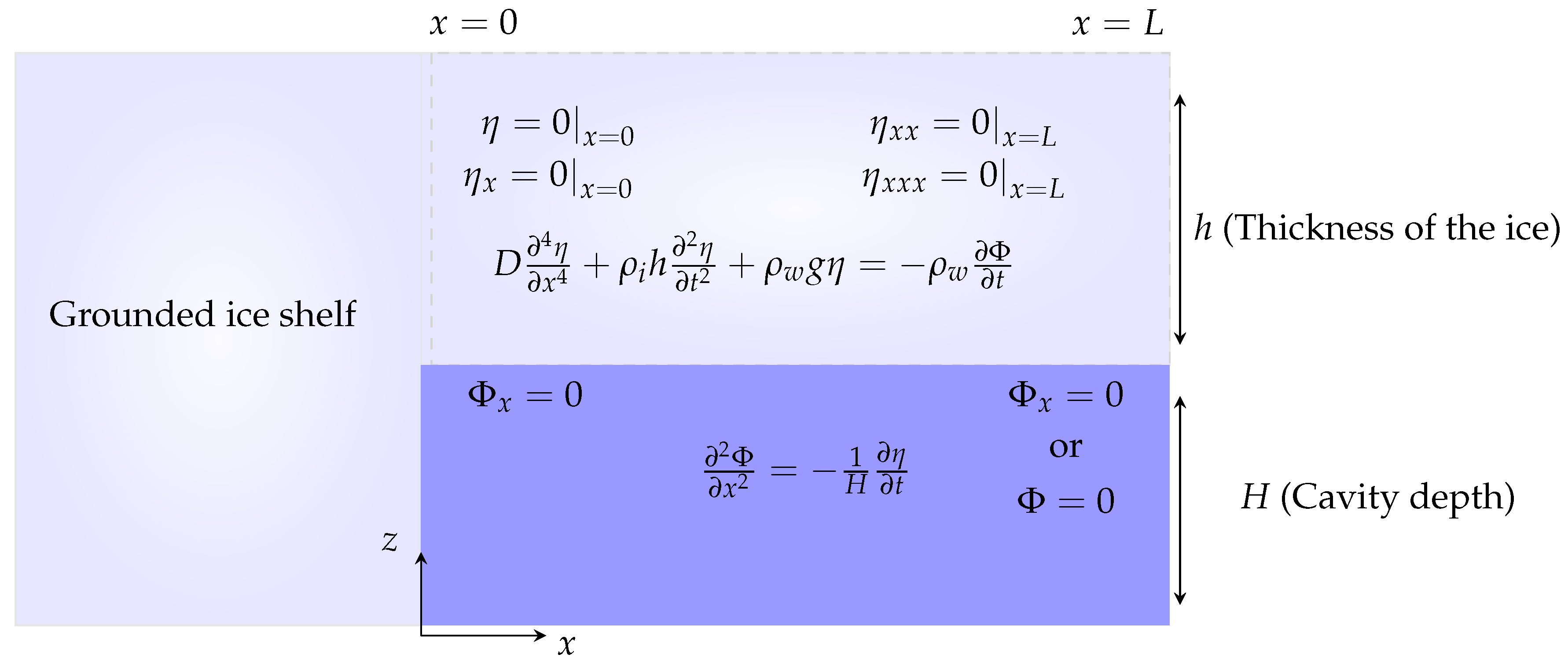
We assume that the motion of the fluid can be described by a potential function,
, that satisfies the linear shallow water equation [
29]:
where
H is the uniform depth of water below the ice shelf, and
is the displacement of the ice shelf. The standard assumption [
18,
19] is that there are no-flux conditions at the ends of the cavity, which means that
In what follows, we will also consider what may be a more realistic assumption that the pressure at the seaward end is zero, following the work in [
28], that is,
The thin plate approximation is used to model the displacement and flexure of the ice shelf:
where
g is the acceleration of gravity
; the length of the ice shelf here is
km, the density of the ice is
, the density of the water is
kg
, and
is the flexural rigidity of the shelf, where
GPa is its effective Young’s modulus and
its Poisson’s ratio. The boundary conditions for the vertical displacement
are given as
The conditions when
at the landward end represent no deflection and no slope, and when
at the seaward end, the bending moment and shear force will vanish. The equations and a schematic are shown in
Figure 1.
The variable
can be eliminated by taking the derivative with respect to
t in Equation (
4) and substituting Equation (
1) to obtain an equation containing only
:
Non-dimensional variables are now introduced following the work in [
19,
30]
where
For clarity, the hats will be dropped from now on.
In the nondimensional variables, Equation (
6) becomes
Equation (
9) depends on the single nondimensional parameter
Note that, for most practical cases,
. The derivation of
M is discussed in detail in [
19,
30]. If we assume
M, we have a nondimensional equation that is independent of any parameters, i.e., it would apply to any ice shelf (obviously, under our assumptions).
Our goal is to find the modes of vibration and use these to simulate the motion of the ice shelf. We begin by determining the time-harmonic solution of Equation (
9), expressed as follows:
Therefore, Equation (
9) can be reduced to one involving
only:
Thus, the general solution has the form of
where
(
) are the roots of
k of the characteristic polynomial:
We now have a typical eigenvalue problem to solve, in which we have six unknowns and six homogeneous boundary conditions, and we must find the values of
for which there are nontrivial solutions. The conditions are as follows:
and either
for the no-flux or
for the no-pressure condition. The no-flux condition assumes that the fluid cannot flow out from the seaward end of the ice shelf. The no-pressure condition assumes that the fluid can flow out but that the pressure remains constant.
3. No-Flux Solution
We begin with the no–flux condition. Enforcing the boundary conditions (
14), (
15), and (
16) at the ends of the ice shelf leads to the system of six linear equations
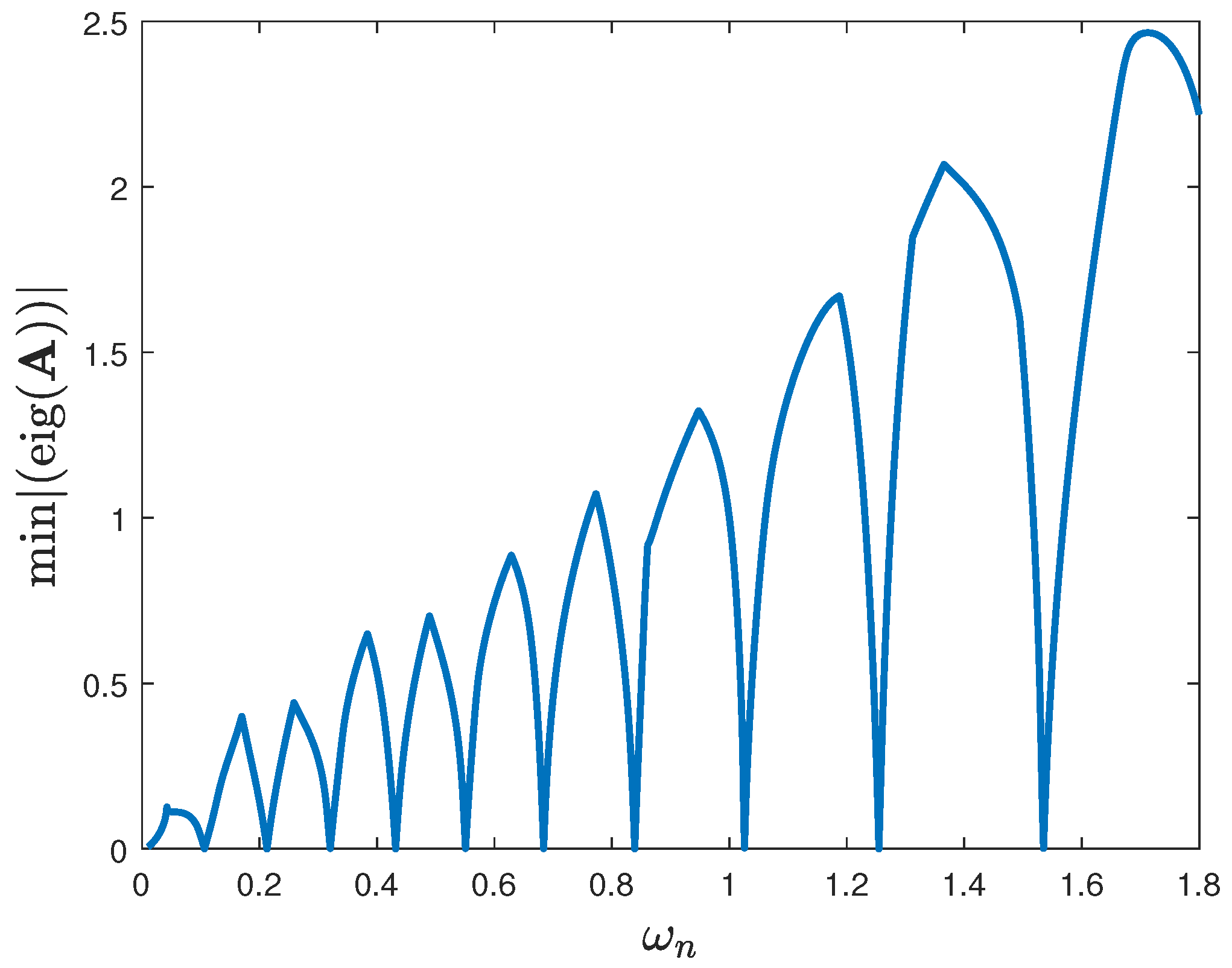
:
Here, in order to avoid the trivial solution, we require the value of to be chosen so that is singular. We solve numerically using the minimum of the absolute value of the eigenvalues of , , and searching for the values of that make this function zero. Once we locate the angular frequency for which is singular, we find the coefficients from the eigenvector associated with the zero eigenvalue.
In the numerical examples that follow, we choose the length of the ice shelf to be
km, the thickness of the ice is
m, and the depth of the cavity is
m following the work in [
19]. This leads to a value of
and a nondimensional length of
.
Figure 2 shows the function
, with the zeros clearly visible.
Table 1 shows the nondimensional angular frequencies
and the dimensional periods
. These values match those previously found in [
19]. We also investigate the significance of the term
M. When
, the longest period occurs when
h with
. Furthermore, the longest period when
occurs at
h with
. As the mode number increases, the periods for
and
decrease significantly while the angular frequencies increase. We can only see a slight difference between
and
for the lowest frequencies. The effect of non-zero
M increases with frequency as expected due to the
term in Equation (
13).
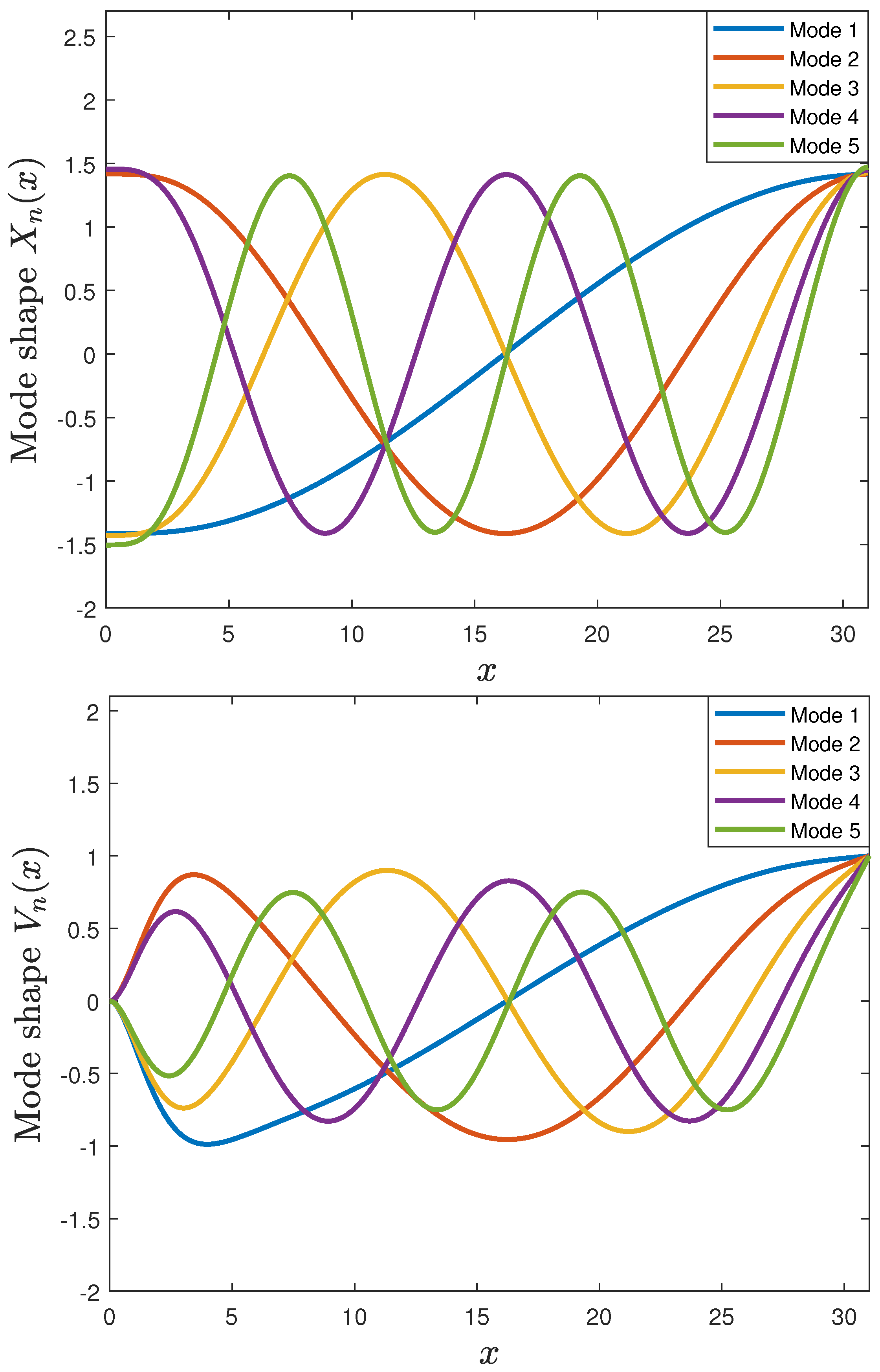
The associated mode shape for the potential is given from the zero eigenvector
as
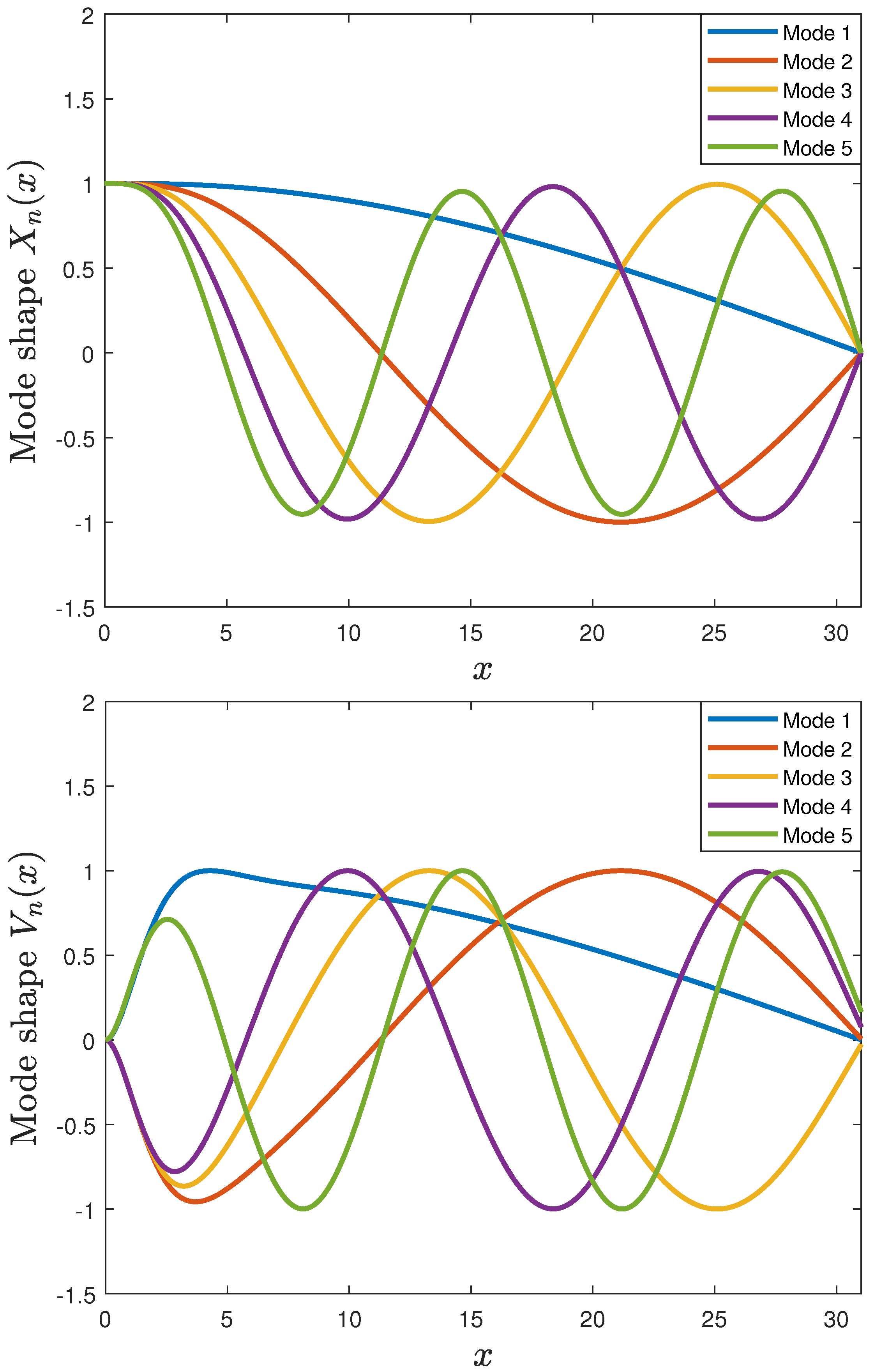
Figure 3 shows the first five mode shapes of
. For the vertical displacement, the time-harmonic solution is given as
To find the mode shape in displacement, we use Equation (
1) to construct the vertical displacement of the potential velocity. We have
So, the mode shape equation for the vertical displacement is given as
Figure 3 shows the shapes of the first five modes of
and
in nondimensional units. We believe that these eigenvectors belong to a generalization of Sturm-Liouville theory, and they can be seen to share many properties. In particular, the number of nodes increases by one each time the mode number increases.
4. No-Pressure Solution
Here, we apply the no-pressure condition at the free end, whereas the clamped end still has the no-flux condition, similar to the work in [
28]. Note that although this boundary condition was not considered by [
18,
19], the results of [
28] indicate that it more closely matches the open water boundary. Enforcing the boundary conditions (
14), (
15), and (
17) at the ends of the ice shelf leads to the system of six linear equations
as follows:
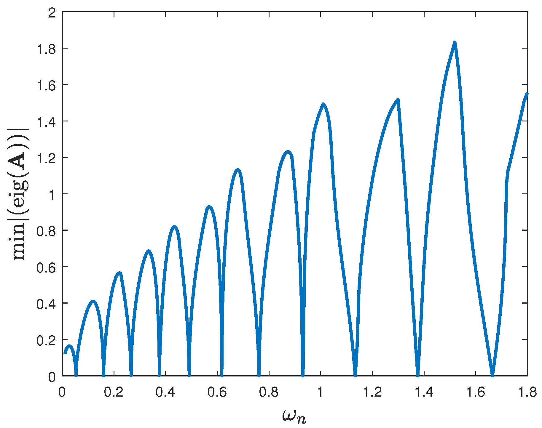
As was the case before, we require
to be singular to avoid the trivial solution. We find the coefficients
from the corresponding zero eigenvector.
Figure 4 shows, again, how we search for the critical values of
, as we did previously.
Table 2 shows the dimensional periods,
, associated with nondimensional angular frequencies,
, for the same case considered in
Table 1, except for the no-pressure case. When comparing
Table 1 and
Table 2, we see that the periods are significantly lower for the no-pressure case compared to the no-flux case. This is further shown in
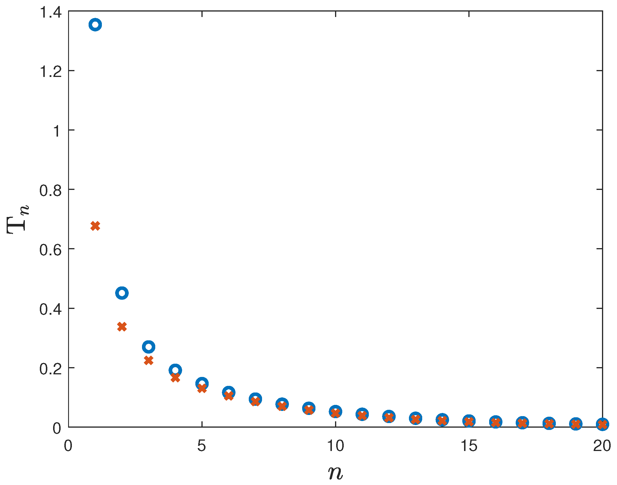
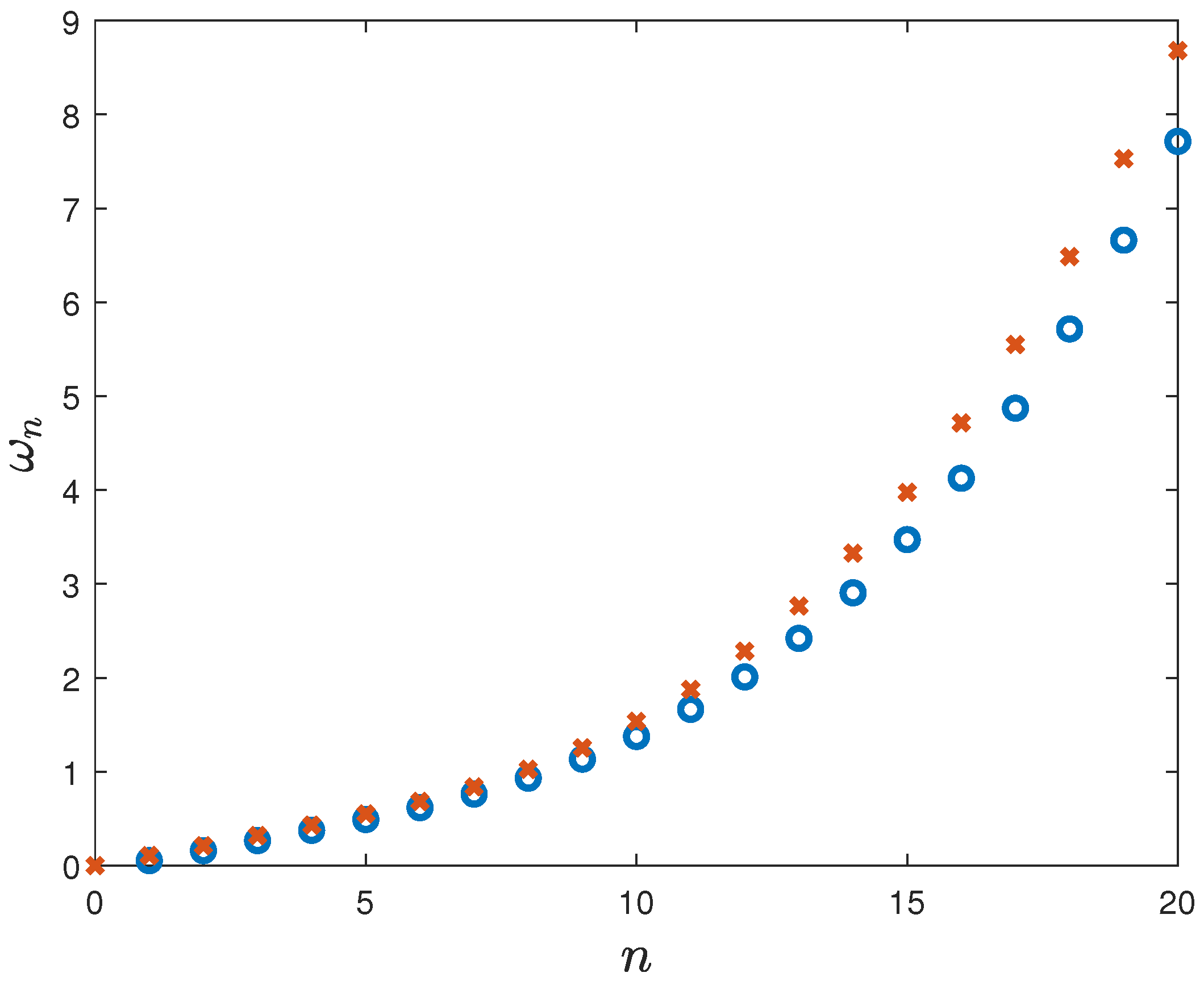
Figure 5 and
Figure 6, which compare the 20 longest periods for the two cases. We can see that the periods and frequencies seem to lie between each other.
Figure 7 shows the first five mode shapes of
and
for the no-pressure case. Note that they are calculated using Equations (
19) and (
22), as before.
Missing Mode for the No-Flux Case
We can see from
Figure 7 that the lowest mode for the no-pressure case has no nodes. In contrast, the lowest mode for the no-flux case (
Figure 3) has one node. This indicates that there is a missing mode for the no-flux case. This missing mode is the nontrivial solution for
, with the corresponding mode
.
5. Simulating Ice Shelf Vibrations
The main aim of the present work is to use the modes to simulate vibration in the time domain. The potential,
, is expanded in terms of the modes as
where
depends on the initial value of
at time
, and
depends on the initial time derivative of
. Note that for the case of no-flux, the sum of the first term begins at zero.
For the vertical displacement, the general solution is given as
where
depends on the initial position at time
, and
depends on the initial velocity.
Note that the sum begins at one for the displacement in both cases. This means that the initial value of the displacement is restricted. Equation (
1) must be satisfied so that
Thus, in the case of the no-flux condition, the right-hand side of Equation (
26) will vanish. Since this equation applies to each mode, it follows that
Note that this is not the case for the no-pressure condition. This issue is linked to the
solution for the potential in the no-flux case. The associated mode,
, cannot be used in the calculation. There is a physical explanation for this: the total fluid under the ice shelf must be conserved (since it is incompressible and cannot flow out) under the no-flux condition. Therefore, when choosing the initial value for displacement for the no-flux conditions,
must satisfy the condition
In the case of no pressure, there is no such restriction. A similar argument shows that the initial condition for the time-derivative of pressure under the ice shelf must also satisfy a similar condition, as does the time-derivative of displacement for the no-flux case. This point was mentioned in [
20] in the context of very large floating structures in an enclosed basin.
Find the Coefficient in the Expansion
Consider the case where we want to determine
so that Equation (
24) satisfies the initial conditions
and
. This implies that
By multiplying both sides of Equation (
29) by
and then integrating the result, we obtain
We note here that the modes
are not orthogonal with respect to the standard inner product. It may be possible to find a function space in which they are orthogonal, but we were not able to do this. For this reason, we use a numerical method. We approximate the integrals by numerical quadrature as
where
are
N-evenly spaced points between 0 and
L (note that more complex spacing could be used), and
is the associated weight function for the quadrature (we use the trapezoidal rule). We then introduce the following matrix:
and vectors
,
, and
. Then Equation (
31) becomes
where diag means the diagonal matrix formed from the vector and the superscript
T is the matrix transpose.
We can then write the solution for potential (Equation (
24)) in the same discrete form (that is, at the points
) as
which gives a very efficient method to calculate the time-dependent motion once the modes have been calculated.
The same method works when calculating the solution for a non-zero initial time derivative of the potential or for the displacement.
6. Results
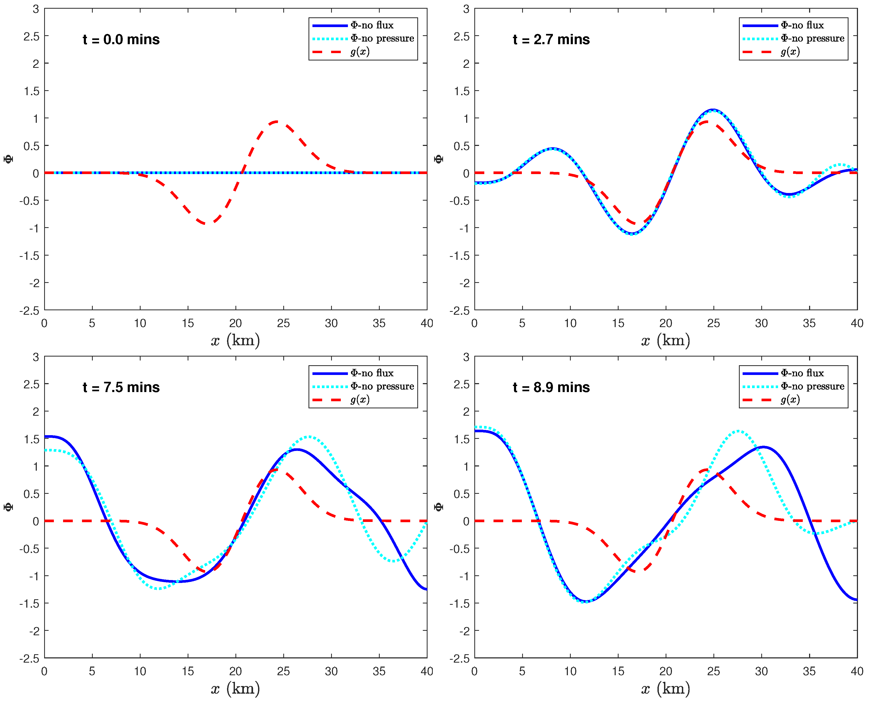
We present simulations of the ice shelf motion in the time domain. These are best viewed in the movies provided in the
Supplementary Materials. We begin by simulating the potential velocity,
.
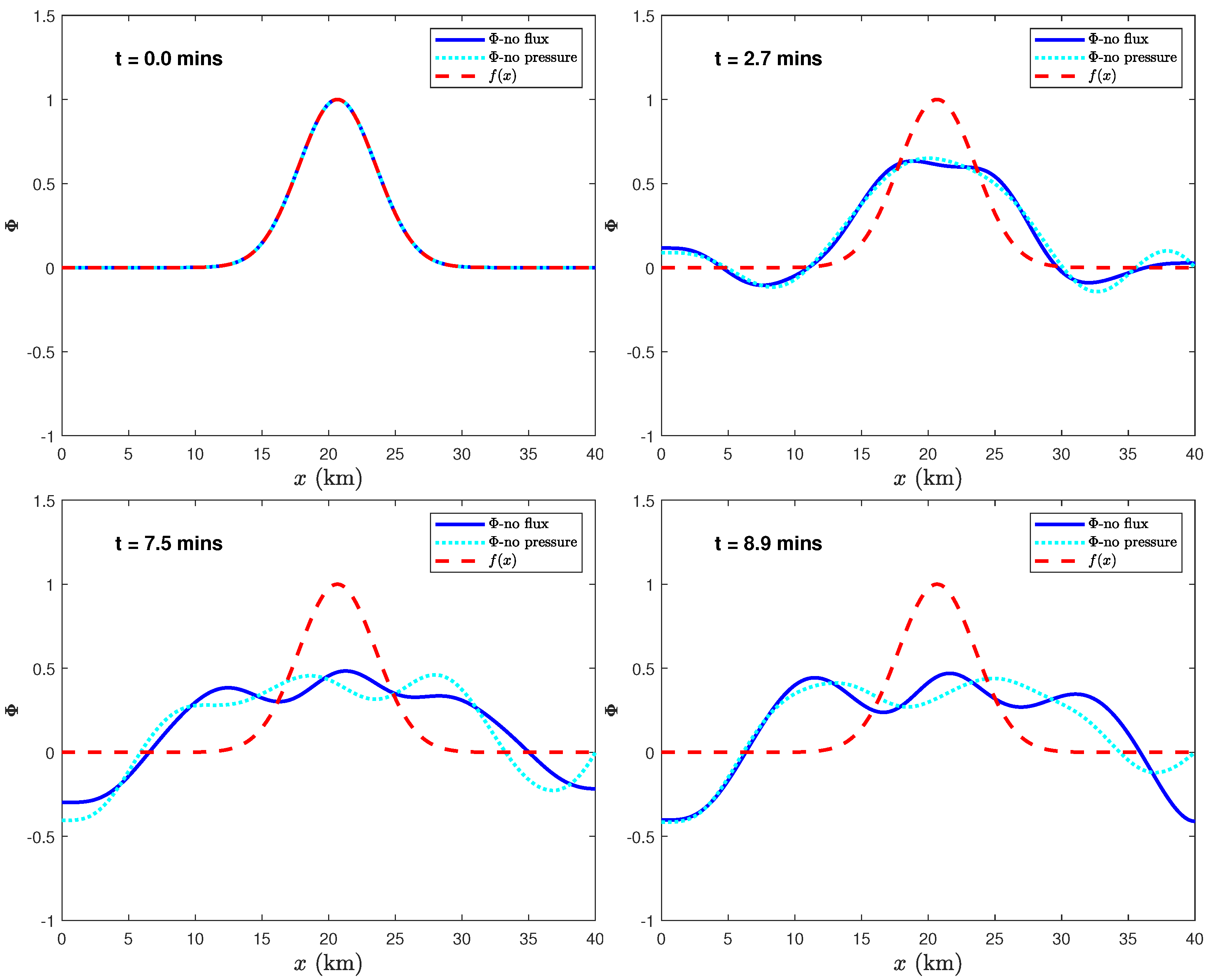
Figure 8 shows the simulation of the solution for Equation (
24) when we apply the initial conditions
and
. We can see the case of no-flux (blue) and no-pressure (cyan), as well as the initial
function (red). Here, we take a Gaussian function:
Figure 9 shows the simulation of the solution for Equation (
24) when we apply the initial conditions
and
. Where
It can be seen in
Figure 8 and
Figure 9 that the solution matches the boundary conditions for the case of no pressure (cyan).
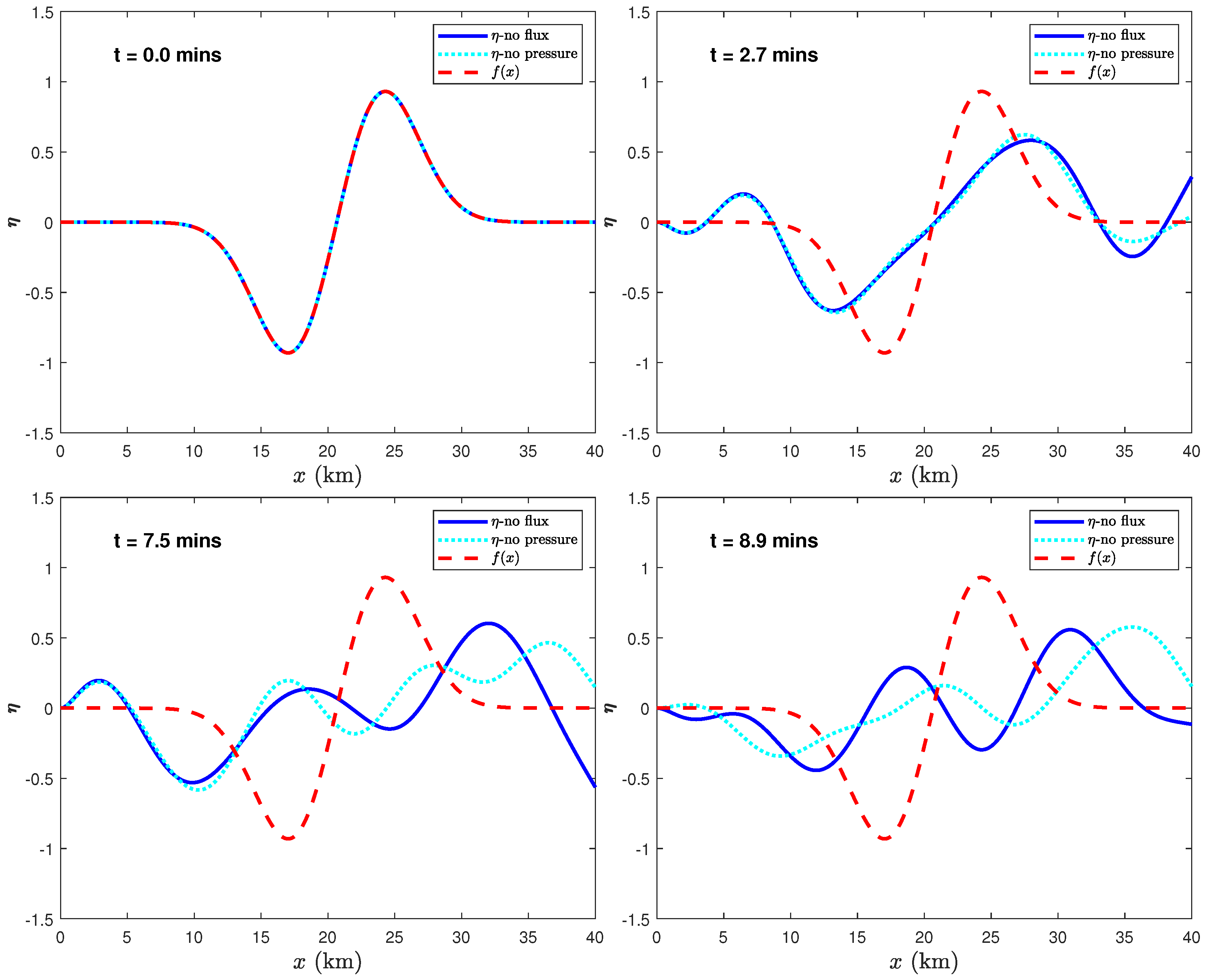
On the other hand,
Figure 10 shows the solution for Equation (
25) when we apply the initial conditions
and
. The vertical displacement,
, for the case of no-flux (blue), the case of no-pressure (cyan), and the initial function
(red) are shown. Note that
was carefully chosen here to satisfy Equation (
28):
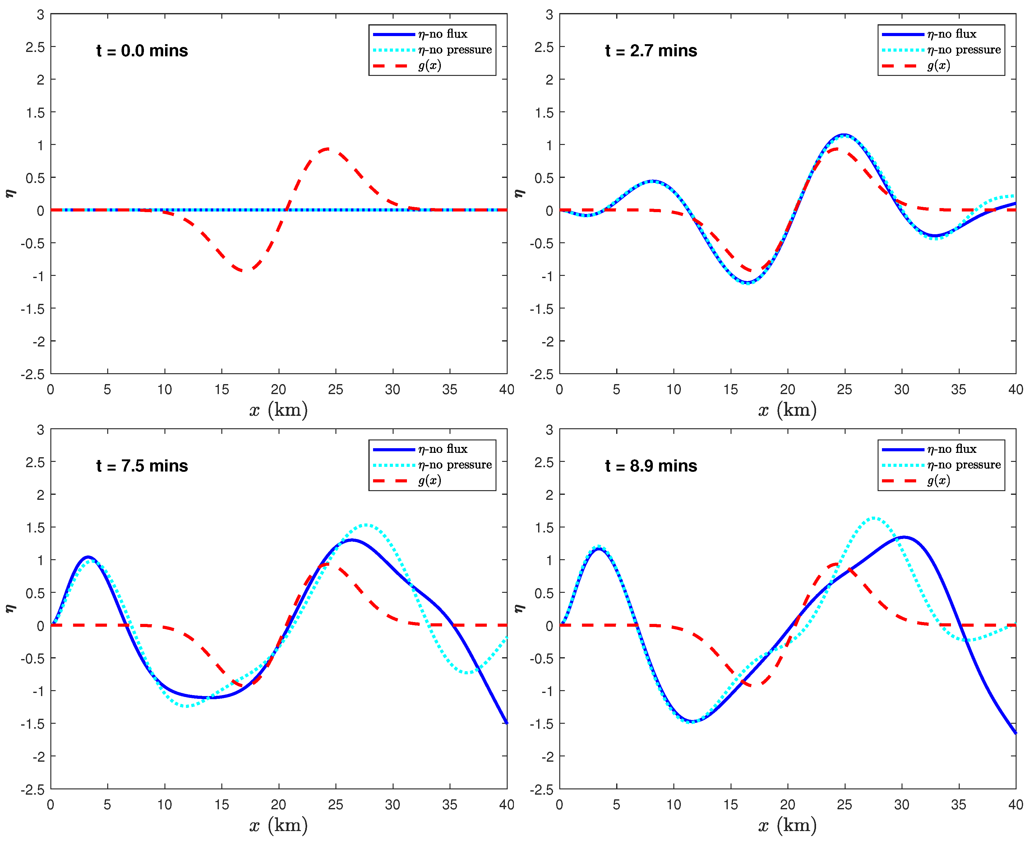
In addition,
Figure 11 shows the solution for the vertical displacement when we apply the initial conditions
and
. Here, we take the difference of a Gaussian so that the integral of the function vanishes:
We can see from
Figure 10 and
Figure 11 that the simulations of the solution match the boundary conditions (
5).
The figures of motion and, more particularly, the accompanying animations of the ice shelf simulations show a complexity that appears to be similar to random processes but is actually based on deterministic principles. The sixth-order equations that model this motion introduce a great deal of complexity in the ice shelf dynamics. Moreover, in reality, our model is a simplified version of a real ice shelf, and we can anticipate it to display even more intricate motion. The intricate deterministic nature of the governing equations implies that a single measurement may not provide a thorough understanding of the wider dynamics. This has implications for the interpretation of point measurements of ice shelf motion.
7. Conclusions
We have explored the time-dependent oscillations of an ice shelf. The solution was constructed by expanding the motion in the mode shapes, which are the eigenfunctions of the system, each of which is associated with an eigenfrequency. In the literature, two energy-conserving boundary conditions have been considered: no-flux, which is more prominent, and no-pressure. The two solutions qualitatively give the same motion, although the no-flux condition can only be used to simulate initial conditions with an integral of zero. We presented time–domain simulations of the solutions for both no-flux and no-pressure cases. The corresponding motion is very complicated, and while deterministic, it has somewhat random or unpredictable behavior due to the sixth-order nature of the equations. This complex motion, arising here in a very idealized model, indicates that actual ice shelf motions will be extremely complex and difficult to interpret from single spatial point measurements of the response. Future work will look to extend this model to three dimensions and include the effect of cracks or other sources of non-uniformity.


