Abstract
This study examines the hydrodynamic regimes in Shediac Bay, located in New Brunswick, Canada, with a focus on the breach in the Grande-Digue sand spit. The breach, which was developed in the mid-1980s, has raised concerns about its potential impacts on water renewal time and water quality in the inner bay. The aims of this study, using mathematical modeling approaches, were to evaluate the flow regimes passing through the breach and influences on the distribution of dissolved matter, providing insights into whether the breach should be allowed to naturally evolve or be artificially infilled to prevent contaminant stagnancy in the bay. The study considered three simulation scenarios to comprehend the water renewal time and the role of the breach in the environmental management of Shediac Bay. Results indicated that completely closing the breach would significantly increase the water renewal time in the inner bay, although the spatial extent of this increase is limited. However, the study identified some limitations, including the need to better define the concentration limit for considering water as renewed and the lack of consideration of dynamic factors such as wind and wave effects.
1. Introduction
The coast of the Gulf of St. Lawrence along the province of New Brunswick (including Chaleur Bay and Northumberland Strait) comprises several sand spits and barrier islands [1,2,3,4,5]. These coastal features shelter back bays which may harbor mollusk aquaculture and fisheries, important activities for the local and provincial economy, with an exportation value of $2.21 G in 2021 [6,7,8,9], but which require good water quality and specific environmental conditions [10,11].
The use of mathematical modeling for the environmental management of the water quality in these sheltered bays, especially of the residence time simulation influenced by tidal cycles and the openness level of water bodies, is extremely indispensable. A couple of studies in the extant literature, including Guyondet et al. (2005) and Deb et al. (2022), are very relevant to this issue but not sufficient to describe the hydrodynamic complexity of sheltered bays such as Shediac Bay (SB) in southeastern New Brunswick, Canada [12,13]. A more robust approach with validation of real-time data is urgently needed, particularly when little data is available, to proceed with a preliminary study before undertaking a full modeling procedure.
Shediac Island and the Grande-Digue sand spit shelter the inner bay from the more energetic waves of the Northumberland Strait (Figure 1). In this area, American oysters, blue mussels, soft-shelled clams, and quahogs are part of the benthic community, and shellfish harvesting is widespread while oyster farming is under development in the inner bay [14]. However, the development of a breach in the Grande-Digue spit in the mid-1980s [15] has raised concerns from fishers, bivalve farmers or aquaculturists, and coastal property owners. It was followed by several attempts to fill it or prevent its widening to ensure that the protection provided by the spit is maintained. It was only in 2019 and 2020 that a project was developed to restore the Grande-Digue sand spit, but since its emergence the breach has progressively widened to reach 410 m wide, though it is still shallow. Impacts from its presence have been reported by local operators such as fishers, mollusk farmers, as well as residents, and have included the following: seasonal or event-related variations in water temperature; seaward and landward sand transfer through the breach, leading to the hardening of the sea bottom in the inner bay and to the loss of shellfish habitats through sand burial; and exposure of the inner coast to higher energy waves.
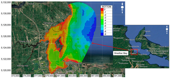
Figure 1.
Delineation of the study limits (Grande-Digue–Northumberland Strait), modeled area and its bathymetry (the color scale, in meters).
While the local population and fishing industry support the restoration of the Grande-Digue sand spit, questions have been raised about possible impacts on the water renewal time in the inner bay following a closure of the breach, which could modify the water quality in this part of SB [12]. As the Department of Fisheries and Oceans of Canada (DFO), which supports the project through its Coastal Restoration Fund program, requests a review of any “project near water”, a preliminary modeling of both the impact of the closure and absence of the closure of the breach on the water residence time has been performed, including the part of SB which is presently protected by the sand spit. It was based on data gathered by recording devices provided and installed by DFO but did not include any sampling for tracer elements, as funds could not cover expenses for personnel and analyses at this stage.
The main objective of this study focuses on the investigation of the flow regime of the sheltered Shediac Bay. Due to the hydrodynamic complexity of this bay and the limited availability of real-time data, we decided to use the open-source TELEMAC software (version v7p2r0) due to its robustness and flexibility in incorporating other coding sources [16,17]. Three simulation scenarios are considered to examine the effect of the breach in the flow states, the water renewal time, and potential impacts on the distribution of the dissolved matter, which will then be estimated via a mathematical modeling approach. The ultimate goal of our simulation is to define the role of the breach in the environmental management for the bay and to answer the question of whether or not the breach should remain evolving naturally or be artificially infilled (restoration of the sand spit), due to the potential of contaminant stagnancy within the bay.
2. Methodology
2.1. Study Area
Shediac Bay is located 24 km to the east of the Moncton–Dieppe–Riverview conurbation, the largest urban area in New Brunswick (total population of 128,168 according to the 2021 Canada Census, Statistics Canada). Its surface area at high water mark is 50.6 km2 and its volume is 101 × 106 m3 (CD). The Scoudouc River and Shediac River are its two main fresh water sources, with mean monthly freshwater discharge rates in the bay ranging from 31.1 ± 11.2 m3/s in April to 2.4 ± 2.2 m3/s in September [18]. The tides follow a diurnal and mixed regime, and the tidal range is microtidal (0.8 m mean tide, 1.3 m high tide) (extracted from the 2021 Canadian Tide and Current Tables). The tidal volume of SB at mean tide is 35.4 × 10⁶ m3, the flushing time is 41.2 h, and the tidal/freshwater volume ratio is 167.95 [18].
The bay and adjacent coast of Northumberland Strait have experienced sustained demographic and urban development in the last few decades, which is associated with the extension of coastal hardening and increased interference with the coastal dynamics [19]. In our study area, this has led to the modification of the longshore drift, the destabilization of the Grande-Digue sand spit, and, ultimately, to the initiation of the present breach in 1985 (Jolicoeur and O’Carroll, in prep.). Urban and economic development in the Shediac Bay watershed since the 1980s may also have changed the amount and nature of nutrients and other chemicals that enter the bay [14]. One of the issues that we must deal with is to make sure that the closure of the breach would not cause unwanted impacts on fishing activities in the inner bay because of the restoration of the sand spit.
2.2. Delineation of the Modeling Area and Bathymetry Data
The limits of the modeled study area were defined based on the available bathymetric data provided by DFO, as well as based on boundary conditions of the area of interest. Moreover, these limits must also satisfy the criterion to encompass selected observation stations within the modeling area in order to use their data for calibrating and validating the hydrodynamic models.
Figure 1 represents the study area boundaries for this project. The study area includes one offshore boundary and two river boundaries (the Shediac and Scoudouc Rivers).
All elevation data presented here are expressed in the Canadian Geodetic Vertical Datum of 2013-CGVD2013. Based on the available and collected data, the bathymetry in Shediac Bay varies from −9 m to 1 m, but only from −3 m to 1 m within the inner bay, i.e., the part of Shediac Bay which is located behind the Grande-Digue sand spit. In Figure 1, bathymetry data are illustrated in red color standing for the highest elevation, and in dark blue color for the lowest elevation. The core modeled area (for calculations) is shown as a dashed circle. It covers about 3 km2 where the depth varies from −2 m to 0 m.
2.3. Governing Equations of the Study
2.3.1. Brief introduction to TELEMAC
TELEMAC is the shortcut name of the open TELEMAC-MASCARET system, a suite of finite element method computer programs for CFD (computational fluid dynamics). This software was conceived, developed, as well as owned by the Laboratoire National d’Hydraulique et Environment (LNHE), part of the R&D group of Électricité de France [16]. After many years of commercial distribution, a consortium (the TELEMAC-MASCARET Consortium) was officially created in January 2010 to organize the open-source distribution of the open TELEMAC-MASCARET system. The latter is a hydrodynamics module, essentially conceived to solve the so-called shallow water equations by using the finite element method or finite volume method with a computational mesh of triangular elements. It can perform robust simulations in transient and permanent conditions.
TELEMAC can help researchers in hydrodynamic backgrounds with the following complex phenomena in many fields of application such as the non-linear effects of propagation of long waves, turbulent flows, bed friction, and the influence of meteorological factors: atmospheric pressure and wind, dam breaks, flood studies, transport of dissipating or non-dissipating tracers, and many others [16,17].
2.3.2. Mathematical Formulation
We expect to simultaneously solve the following hydrodynamic coupling equations:
Continuity equation:
Momentum equation along the depth h:
Momentum equation along x:
Momentum equation along y:
Mass conservation equation for tracers or dissolved matter:
Eulerian passive tracer experiments are widely applied in estimating renewal timescales [20]. The governing equation for tracer concentration is as follows:
in which:
h [m]: depth of water;
u,v [m/s]: velocity components;
[m/s2]: gravity acceleration;
[m2/s]: momentum diffusion coefficients;
Z [m]: free surface elevation;
t [s]: time variable;
[m]: horizontal space coordinates;
Sh [m/s2]: source or sink of fluid;
Sx, Sy [m/s2]: source or sink terms in dynamic equations;
C [g/m3]: concentration of tracers or dissolved matter;
U [m/s]: vector of flow velocity, U = U(u,v,z).
x, y, and z are the three-dimensional spatial coordinates within the model (m); u, v, and w are the velocity in the x, y, and z directions (m/s), respectively; DN is the vertical turbulence diffusivity (m2/s), used in temperature and salinity calculation as well; DN can also be understood as the coefficient of diffusion of the tracers of dissolved matter; and Fh is the horizontal diffusion term (concentration/s). Generally, tracers are placed inside the bay or in estuaries/lagoons, and the way in which concentrations decrease over time is modeled.
It is noted that while Equations (2)–(4) are expressed in the two-dimensional format, Equations (1) and (5) are in the general 3D form. The h variable in this case is the average value of water depth to be introduced into the system which is reduced to the 2D problem, hence the use of TELEMAC2D software (version v7p2r0).
2.4. Input Data
Three groups of data were used for our simulations:
- Bathymetry data: provided by DFO, Gulf Region (combining a Lidar data set covering most of the inner bay [21] and CHS non-navigational 100 m data for deeper offshore areas [22]);
- Atmospheric data: retrieved from the nearby ECCC meteorological stations in Moncton and Bouctouche [23];
- Hydrological data: this type of data was collected at 9 different observation stations within the study area to measure various parameters that served for the model calibration and validation. Stations were equipped with Onset HOBO U20 pressure loggers (water level), Sontek Argonaut-XR and RDI Workhorse acoustic Doppler current profilers (current direction and velocity), and Sea-Bird Microcat sensors (water temperature and salinity). Figure 2 shows the location of these nine observational stations (image on the left-hand side) and measured parameters at each station (table on the right-hand side). There were three measured parameters adopted for our calculation and validation steps, including water level, current velocity, salinity, and meteorological data.
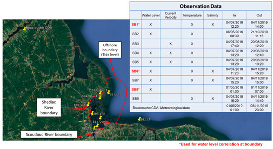 Figure 2. Observation stations and observed parameters (water level, current velocity, temperature, and salinity).
2.5. Modeling Framework
2.5.1. Meshing
Meshing is a mandatory step for the simulation of fluid dynamics problems. The process of mesh generation plays a critical role in ensuring the accuracy of simulation results. Our meshing system herein includes an unstructured triangular mesh generated in BlueKenue Software (version 3.9.3), which is an advanced data preparation, analysis, and visualization tool for hydraulic modelers [24]. The final mesh used in this study comprises a total of 19,683 nodes and 37,392 elements. The average distance between two nodes is 200 m in the offshore part of the mesh and 20 m in the coastal areas, especially for the core of calculation within the study site (limited by the dashed circle in Figure 1).
It is noted that the choice of meshing resolution is totally dependent on our simulation objectives. We targeted the hydrodynamic regimes and water renewal time simulations in the inner bay. Therefore, to minimize errors as much as possible, the choice of a finer mesh for this area had to be made. Otherwise, the outer area such as the offshore part used a coarser mesh so that we could save more time on computation without impacting the accuracy of the results. Due to the scope of this study, we only focused on the water renewal time calculation and the removal of the sand spit; therefore, all the details of the meshing procedure could not be shown in this paper. Figure 3 shows our adopted meshing system for all calculations hereafter, with the finest mesh centered around our study site (main study area).
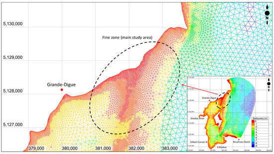
Figure 3.
Calculation mesh for the entire domain and the finer mesh at the main study area.
2.5.2. Model Setup
We applied a 2D depth-averaged hydrodynamic model (with the solver TELEMAC) to simulate the flow regimes in Shediac Bay. The computation domain was designed in order to cover the main study area as indicated with the grid of elements and nodes in Figure 3.
There were two sources of input boundaries used in our simulations: (1) salinity at the offshore area (station SB1) and at the Shediac and Scoudouc Rivers (stations SB6 and SB9); and (2) tidal fluctuation at the offshore area (SB1) and at these two river boundaries (stations SB6 and SB8). Data for salinity and water level fluctuations were collected during the period from 5 July to 4 November 2019, including fully observed data from the Dorian storm on 7 September 2019 (UTC).
The hydrodynamic model was calibrated and validated first using the observed data to ensure good agreement between simulated results and observed data, and was then applied to simulate the renewal time.
A virtual system of tracers was used for our simulation and calculation of renewal time in the inner bay. The turnover time (TT), which is widely used in environmental assessments for aquaculture, can be estimated. It is defined as the time when 1–1/e (~63.2%) of the initial amount of tracer mass in the embayment is replaced with seawater [13,25,26], based on the assumption that the embayment water decreases exponentially over time [27].
Hence, the initial condition of the tracer concentration for this simulation was set at 1 mg/L. There were also two types of initial conditions applied in this research (as presented in Figure 4):
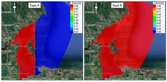
Figure 4.
Applied initial conditions in the model: (Left) Type A and (Right) Type B.
- Type B: Tracer concentration is set up to equal 1 for the entire domain (represented in red color in Figure 4-right), and zero at the boundaries.
A decreasing concentration in time and space is indicative of water renewal in the considered area, understood as being replaced by water from outside with 0 mg/L concentration. Once the simulation terminates, the concentration evolution is examined in each grid cell to determine the last time step at which it has dropped to or below (1/e) its initial concentration [25], where e is a mathematical constant or Euler’s number, approximately equal to 2.71828. In this case, the lower limit of concentration was approximately 1/e = 0.368 mg/L (it is not the value obtained by simulation). This limit can be considered as the threshold at which when the obtained concentration is lower, the considered quantity of water will be replaced by the new water quantity. Water renewal time was then calculated at these cells. The time scale is usually defined as the e-folding time, i.e., the time required to decrease the concentration of the initial tracer to 1/e of its initial value. e-folding time is used in water renewal time simulations because it can provide a simple and effective way to model the rate at which water quantity is replaced by another quantity.
Three scenarios of the simulation of water renewal time included the following:
- A current condition, where the flow regimes passing through the existing breach are generated by the hydrodynamic conditions of the bay without wind and wave effects;
- We assume the breach (following a restored beach and dune) will be totally closed, where water cannot flow into the inner bay through the breach anymore;
- Without any restoration measure, the breach is assumed to enlarge and, at one point in time, to reach a depth of −2 m (based approximately on the adjacent areas) in order to avoid shock waves, i.e., there would be more water traveling into the inner bay from offshore than at present.
2.5.3. Calibration and Validation
Evaluation of the Model Accuracy
The accuracy of our results can be evaluated via the following approaches: (1) standard regression; (2) dimensionless technique; and (3) error indices.
Standard regression can be used to determine the strength of the linear relationship between simulated and measured values, while the dimensionless technique will provide a relative model evaluation assessment; error indices help in quantifying the deviation according to the units of the data of interest [28].
Some common error indices for the discrepancy between simulated and measured data will be used including Mean Square Error (MSE), Root Mean Square Error (RMSE), RMSE-observations standard deviation ratio (RSR), and Percent Bias (PBIAS) (see Table 1, Table 2, Table 3, Table 4, Table 5 and Table 6) [28,29].

Table 1.
Residual indices of the water level in the model calibration.
Table 2.
Residual indices of the current velocity in the model calibration.
Table 3.
Residual indices of the salinity in the model calibration.
Table 4.
Residual indices of the water level in the model validation.
Table 5.
Residual indices of the current velocity in the model validation.
Table 6.
Residual indices of the salinity in the model validation.
MSE and RMSE indicate the errors in the units (or squared units) of the constituent of interest, which aids in the analysis of the results. When MSE and RMSE are equal to 0, these indices show a perfect fit of the model.
RMSE-observations standard deviation ratio (RSR) is defined in the following equation as the ratio of the RMSE and the standard deviation of measured data:
RSR incorporates the benefits of error index statistics and includes a scaling/normalization factor; therefore, the resulting statistics and reported values can apply to various constituents. RSR varies from the optimal value of 0 (which indicates zero RMSE or residual variation, and therefore perfect model simulation), to a large positive value. Lower RSR (and RMSE) values indicate better model simulation performance.
Percent Bias (PBIAS) measures the average tendency of the simulated data to be larger or smaller than their observed counterparts [28]. PBIAS is calculated by the following equation:
The optimal value of PBIAS is 0.0, with the low-magnitude values indicating the accurate simulation of the model, and where positive values indicate the underestimated bias while negative values stand for the overestimated bias [28].
The series of figures from Figure 5, Figure 6, Figure 7, Figure 8, Figure 9 and Figure 10 is shown to provide a visual comparison of simulated and measured data for the model performance. Due to our data, which can be positive and negative, it should be noted that the (qobs) in the denominator of Formula (8) is under the form of absolute value to avoid the ith division by a zero sum.
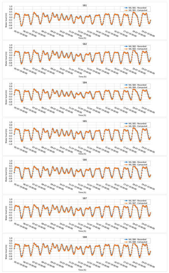
Figure 5.
Model calibration: comparison between the computed and observed water level.
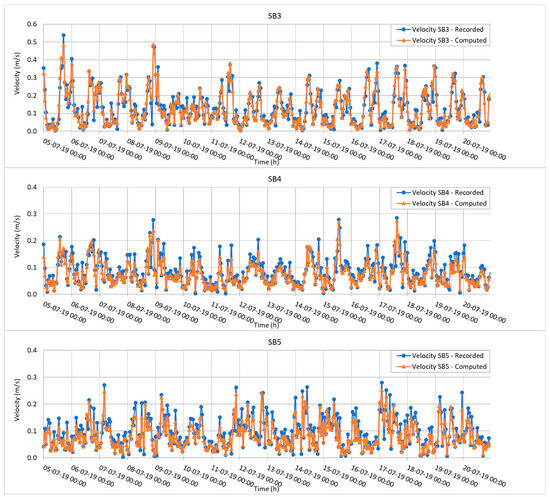
Figure 6.
Model calibration: comparison between the computed and observed current speed.
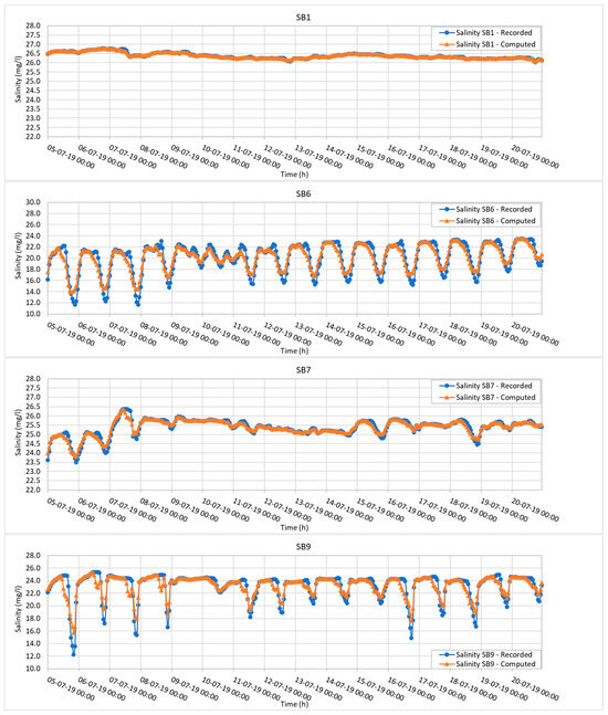
Figure 7.
Model calibration: comparison between the computed and observed salinity.
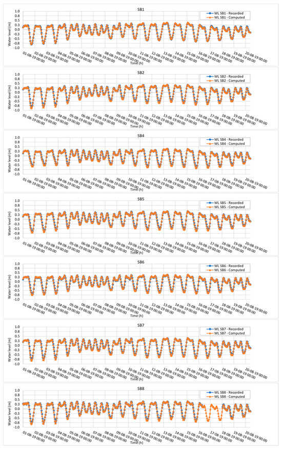
Figure 8.
Model validation: comparison between the computed and observed water level.
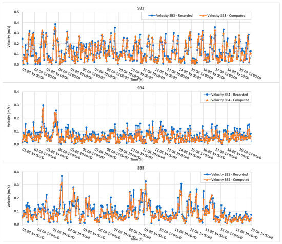
Figure 9.
Model validation: comparison between the computed and observed current velocity.
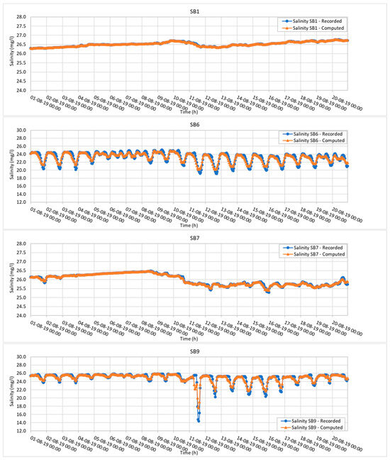
Figure 10.
Model validation: comparison between the computed and observed salinity.
Model Calibration
The model calibration was processed based on the change of bottom friction values in order that calculated results could meet observed data. The advection and diffusion coefficients of the tracer (salinity used in this case) were included in the process to calibrate the transport model.
Our model was successfully calibrated with data from 5 July to 20 July 2019. The calculated results were extracted at nine different locations for comparison with observed data for three various parameters: water level (Figure 5), flow velocity (Figure 6), and salinity (Figure 7).
Based on the comparison between the computed and observed water level in Figure 5, the chart indicates a generally good agreement between the two sets of values. The computed values closely follow the trend of the observed values, with only a few minor deviations. The residual indices calculated are shown in Table 1, providing a reliable simulation of the observed water level, with a high degree of correlation between the two sets of data.
Upon analyzing the comparison chart between the computed and observed current speed in Figure 6, it can be seen that there is a reasonably good agreement between the two sets of values at three locations. The computed values follow the general trend of the observed values, with some residual indices shown in Table 2. In general, the residual indices show that the computed values closely match the observed values.
Figure 7 shows a comparison chart between the computed and observed salinity. It can be concluded that there is a good agreement between the two sets of values, as indicated by the residual indices (Table 3). In this case, the residual indices show that the computed values closely match the observed values, with only a few outliers that can be attributed to measurement errors or uncertainties in the computational model.
Model Validation
Once calibrated, the model was validated by using another period of input data. The validation of the model ensures the performance of all long-term simulations which would be processed later.
The model validation was conducted by using the data for the period from 1 to 20 August 2019. Similar to the Model Calibration section, water level, current velocity, and salinity were also the three parameters used in the validation process. The results have been extracted at nine different locations for comparison with observed data (see Figure 8, Figure 9 and Figure 10 and Table 4, Table 5 and Table 6).
In general, the three charts show that the calculated results are in good agreement with the observed values. Moreover, the residual indices provide a reliable degree of correlation between the two sets of data.
It should be noted that our model was calibrated with the data from July 2019 and validated with the data from the period of August 2019. The model might not be very applicable for all other time periods (especially data series with large variations throughout years), since it was based on a limited and specific dataset. If we expect to use it for any other period data, the model must be revalidated again with more independent data. Therefore, the reliability of measured data is crucial for both calibration and validation processes. In the case of unreliable data, the simulation may run endlessly and produce erroneous results. Overall, the comparison of computed and observed data as well as residual indices suggest that the computational model is valid and usable for further steps.
3. Results and Discussion
3.1. Observations for Hydrodynamic Results in the Current Condition (Scenario 1: “Free” Flow)
Snapshots of the flow distribution (direction and velocity) during typical ebb and flood phases of the tide are presented in Figure 11.
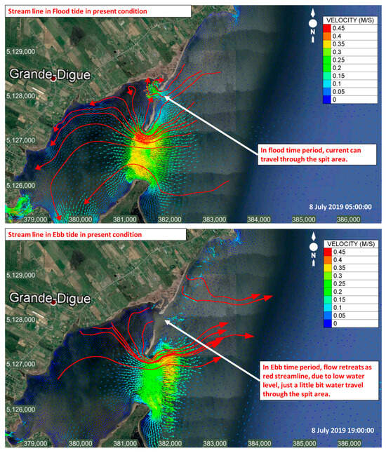
Figure 11.
Velocity distribution and streamlines in the flood tide and ebb tide periods (scenario 1).
The flow speed varies from 0 to approximately 0.5 m/s. There is a considerable difference between flood and ebb tides through the breach area at a low water level, when the tidal flat interferes with the water going through. Based on the streamlines of a flow within the flood tide and ebb tide, it can be seen that there is no flow through the breach in the ebb tide period due to the shallow water level.
3.2. Flow Distribution for the Three Different Scenarios
As previously described in the introduction, three scenarios of flow passing through the breach were simulated: (1) the current conditions; (2) a closed-off breach (the breach assumed to be closed, as planned in the Grande-Digue restoration project); and (3) a deeper breach (conditions that might evolve without restoration, through the erosion of the bed and progressive channelization of tide flows), which we named “enlarged breach” in this simulation exercise.
Figure 12a shows the location of the breach (the area within the red rectangle). The breach was considered as “closed-off” in scenario 2 or “enlarged” in scenario 3. The dimension of the enlarged breach is approximately 400 m in length, 100 m in width, and −2 m in depth (based on the average depth value of the adjacent areas to avoid shock waves). All other conditions remain the same as in scenario 1 except for the bottom elevation in the breach area, which is numerically “modified” according to each scenario’s conditions.
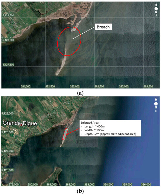
Figure 12.
(a) Location of the present breach; (b) dimension of a modeled enlarged breach (scenario 3).
The flow distribution during a flood tide for these three scenarios is presented in Figure 13. It is observed that the flow distributes wider through the breach in scenario 3 (enlarged breach), whereas in scenario 2, there is no flow through the closed-off breach. Clearly, when the breach is enlarged, more water flows into the inner bay and it is flushed faster.
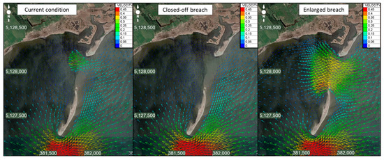
Figure 13.
Comparison of flow distribution in the three scenarios.
3.3. Renewal Time Simulation and Observations
3.3.1. For Type A Conditions
The general (entire) view of renewal time for type A is presented in Figure 14a, while a closer view of the main study area is shown in Figure 14b.
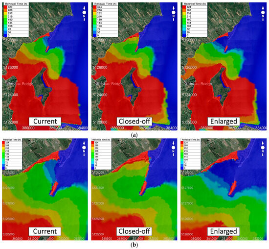
Figure 14.
(a) Entire view of the renewal time for the three scenarios (initial condition type A); (b) closer view of the renewal time at the main study area for the three scenarios (initial condition type A).
Based on the results simulated with initial condition type A, from scenario 1 (current condition) in Figure 14b, the renewal time varies from 36 to 180 h (see the color scale). When the breach is closed-off (scenario 2), i.e., water cannot travel into the inner bay through the breach, the renewal time significantly increases, varying from 144 to 252 h. In an opposite manner, when the breach is enlarged (scenario 3), the tracer will be quickly flushed away in less than 36 h.
3.3.2. For Type B Conditions
The entire and closer views of the renewal time for the type B condition are presented in Figure 15a,b. With the type B condition, it is observed that the renewal time becomes longer. The renewal time (a) varies from around 544 to 688 h for scenario 1 (current conditions) (Figure 15b, see the color scale); (b) increases to 904 h for a closed-off breach (scenario 2); and (c) decreases to approximately 200 h with an enlarged breach (scenario 3).
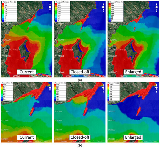
Figure 15.
(a) Entire view of the renewal time for the three scenarios (initial condition type B); (b) closer view of the renewal time at the main study area for the three scenarios (initial condition type B).
With both type A and B initial conditions for the tracer concentration model, the results show a common tendency of renewal time. Simulations indicate that when the breach is closed, the renewal time will increase considerably compared to the current condition, i.e., the renewal time is four times longer. However, the area where water renewal is affected by the breach closure is limited to the inner bay, in the immediate vicinity of the breach itself. For a more precise comparison, we illustrate the renewal time evolution at the random cross section A-A’ (Figure 16a), and a temporal change in tracer concentration at a random location in the inner bay (the blue dot in Figure 16b), in the three scenarios.
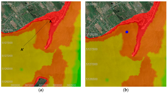
Figure 16.
(a) Location of the random cross-section A-A’ to analyze the spatial changes of renewal time for the three scenarios; (b) location of the point used (blue dot) to analyze the evolution of tracer concentration for the three scenarios.
The comparison of the renewal time at the random cross section A-A’ between the two types of initial conditions is presented in Figure 17. The cross section shows the spatial variation of the renewal time from the inner bay towards offshore. The temporal evolution of the tracer and its difference in the three scenarios using initial condition types A and B are presented in Figure 18a,b, respectively. The temporal evolution of the tracer concentration at a certain point within the inner bay gives a clear picture of how much the changes at the breach site would impact the renewal time. From these graphs, we can see that in the closed-off breach (scenario 2—red line), the renewal time is longer than in the current conditions (scenario 1—blue line), while the opposite is true for an enlarged breach (scenario 3—green line).
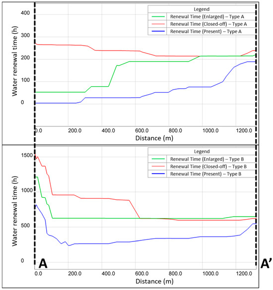
Figure 17.
Comparison of renewal time at the random cross section A-A’ for the two types of initial conditions A and B.
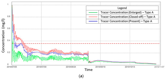
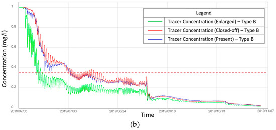
Figure 18.
Temporal evolution of tracer concentration and its difference in the three scenarios: (a) using type A initial condition; (b) using type B initial condition.
It is remarkable to see that there is a numerical jump in Figure 18 in both types of conditions A and B with all three scenarios. This abrupt change can be explained by the fact that there was a strong flushing event following the passage of post-tropical storm Dorian in September 2019 (as previously mentioned in Section 2.5.2), leading to the surge in flow velocities and water levels, hence increasing the total discharge over the studied area. Our numerical simulations can therefore provide the considerable visualization effects of such uncommon storm events on the water renewal of coastal systems. Additionally, it is obviously concluded that the type B condition is more realistic.
3.4. Implications of the Results for the Restoration of the Grande-Digue Sand Spit
This preliminary study was conducted to verify if there is any serious impact to the water quality and to the habitats of commercial species in the part of the inner Shediac Bay that is presently located behind the Grande-Digue sand spit.
The outcomes of this preliminary work indicate that if the breach is totally closed, the renewal time for water in the inner bay could significantly increase, i.e., become much longer in comparison to the time needed in either the current conditions (scenario 1) or if the breach were to enlarge (scenario 3). The spatial extent of the effectual increase is fairly limited. Moreover, the results show that the spatial variation of renewal time is not very significant within the inner bay.
These results will be analyzed by the biologists and marine science specialists responsible for the review of the Grande-Digue restoration project (the “project near water” review). It could result in the authorization to proceed with the restoration plan or identify specific conditions that need to be appeased. Further, the project could lead to advanced reforms in the restoration plan, to avoid or mitigate potential negative impacts on the aquatic ecosystem of the inner bay and its commercial activities. Another possible outcome, if the unknowns are seriously considered, could be necessitating a comprehensive study of the effects of a closure of the breach on the residence time and habitats of benthic and other aquatic species. So, the choice to execute a preliminary study, although mainly caused by a lack of funds, could still be justified.
Regardless of the result after the review by the DFO, local support will continue to depend on a restoration strategy that combines the restoration of the spit and improvements to the present situation. No modeling of the deepening of the breach has been performed to date. The floor still lies in shallow water depth at high tide after more than 38 years (which can easily be traversed by foot during low tide), but if that were to happen, currents and storm waves would obviously change the conditions in the inner bay and at the shoreline. Given the sand transfers, hardening of the base and the loss of mollusk habitats have already been observed beside the breach; hence, the monitoring of its evolution is certainly advisable.
4. Conclusions and Future Perspectives
This study investigated the hydrodynamic complexity of Shediac Bay via the flow regimes which pass through it. The open-source TELEMAC software (version v7p2r0) was used to model three scenarios of flows over the breach, including (1) the current conditions of the existing breach; (2) a closed-off breach (the breach assumed closed, as planned in the Grande-Digue restoration project); and (3) an enlarged breach (conditions that might evolve without restoration, through the erosion of the bed and the progressive channelization of tide flows).
It was observed that the flow distributes wider through the breach in the enlarged breach scenario, whereas in the closed-off breach case, there is no flow going through. Clearly, when the breach is enlarged, more water flows into the inner bay and it is flushed faster.
The renewal time varies from 36 to 180 h with the type A condition. When the breach is closed-off, i.e., when water cannot travel into the inner bay through the breach, the renewal time significantly increases, varying from 144 to 252 h. In an opposite manner, when the breach is enlarged, tracers will be quickly flushed away in less than 36 h. With the type B condition, it was observed that the renewal time becomes longer. The renewal time (a) varies from around 544 to 688 h for the current conditions; (b) increases to 904 h for a closed-off breach; and (c) decreases to approximately 200 h with an enlarged breach. With both type A and B initial conditions for the tracer concentration model, the results show a common tendency of renewal time. The simulations indicate that when the breach is closed, the renewal time will considerably increase compared to the current condition, i.e., the renewal time is four times longer. However, the area where water renewal is affected by the breach closure is limited to the inner bay, in the immediate vicinity of the breach itself.
Based on our simulation results, scenario 2 could be considered as advice for the no-action option, which could eventually lead to the development of a tidal channel and/or to the demise of the present terminal islet. If deemed to conform to the requirements of the Department of Fisheries and Oceans in terms of the ecological integrity of aquatic species and habitats, the Grande-Digue sand spit coastal restoration project will move forwards. This would include the infilling of the breach and the reestablishment of the species and habitats that were present there in 1985. Along an open bay–back bay transverse profile, this would include the grading of a foreshore, a dry beach, an Ammophila-covered sand dune crest, and a Spartina saltmarsh. The outer limits of the project in the bay are set by the present location of healthy eelgrass (Zostera marina) and mollusk colonies. Within these limits, the restoration work has been planned at the current breach location, including the adjacent sea bottom areas impacted by sand transfer from, and through, the breach. Finally, the restoration of the sand spit would include a monitoring program, with the partnership of the local population, to document the integrity and resilience of the infilling, the success of biological reintroductions, and signs of improvement regarding the negative impacts of the breach opening on the economic activities and coastal properties in the back bay since 1985.
All mathematical simulations and the simulation time to reach stable convergence strongly depend on the non-linear nature of equations and initial conditions. The initial condition 1/e represents the bottom of the quasi-linear initial decline in concentration. The choice of this limit conditions the water renewal time absolute values. Using the 1/e value that has been used in previous studies allows for direct comparison with previously reported water renewal time values for other bays.
We have only considered the tidal forces in our simulations, i.e., without incorporating dynamic factors such as winds and waves. A more comprehensive study should combine the simultaneous impacts of winds, waves, and tides, because the directions and intensities of all these factors strongly affect the nearshore flows, which can contribute to the flushing process (and persistence) of contaminants. Such a study is planned in the next step of the simulation to improve the reliability of all the results, especially for the renewal time in an ecosystem without the study of deepening the breach, which has never been conducted in the past.
Using a CFD software to deal with hydrodynamic issues is not new, but the use of TELEMAC simulation in this study was scientifically and practically relevant because we had to face the high complexity of hydrodynamic aspects of the inner bay, simultaneously with the mass conservation system of dissolved matter which is assumed to be conceived for the biological and ecological concepts. Hence, the coupling systems of governing equations on a vast area cannot be solved without the implementation of a robust approach which requires the achievement of several technical skills.
The exclusivity and advantages of using TELEMAC in this study are as follows:
- TELEMAC v7p2r0 is an open-source software, allowing users to access and modify the source to their specific needs, meaning we could operate the CFD tools according to our specific problems at Shediac Bay;
- Generally, in every CFD software, the higher resolution of the computational mesh (very fine mesh) can improve the accuracy and reliability of the simulated results. However, this would require more time and resources for the simulations. Therefore, the benefits from TELEMAC in this study relied on its ability to run simulations in using parallel computing, which is a technique that distributes the computational tasks over multiple processors. This enabled us to save time and resources when running the complex coupling model, which involved both temporal and spatial simulations.
Apart from the applications in the aquaculture and ecology of the bay, the scientific innovation of our findings relies on the resolution of the coupling system of non-linear governing equations with their boundary and initial conditions applied for the real-time data on a sheltered space, which could not be easily executed with conventional coding algorithms and methods. Moreover, this study serves as the first step in our process of merging CFD software for non-linear hydrodynamic equations with GIS/Remote Sensing technology envisaged to soon deal with this category of the problem.
Author Contributions
Conceptualization, C.L., T.N.-Q. and S.J.; methodology, C.L. and T.N.-Q.; software, C.L. and T.N.-Q.; validation, C.L., T.N.-Q., S.J., T.G. and S.O.; formal analysis, C.L. and T.N.-Q.; investigation, C.L., T.N.-Q. and S.J.; resources, T.G. and S.O.; data curation, C.L., T.G. and S.O.; writing—original draft preparation, C.L. and T.N.-Q.; writing—review and editing, C.L., T.N.-Q. and S.J.; visualization, C.L., T.N.-Q. and S.J.; supervision, T.N.-Q. and S.J.; project administration, S.J.; funding acquisition, T.N.-Q. and S.J. All authors have read and agreed to the published version of the manuscript.
Funding
SJ acknowledges the financial support provided by the DFO Coastal Restoration Fund (Contribution Agreement No. 18-HGLF-00331). TNQ acknowledges the NSERC Discovery Grant RGPIN 03906.
Institutional Review Board Statement
Not applicable.
Informed Consent Statement
Not applicable.
Data Availability Statement
Necessary data can be provided by requests.
Acknowledgments
We wish to thank Dominique Bérubé, coastal geomorphologist at the Department of Energy Development and Natural Resources of New Brunswick (Bathurst, NB, Canada), for providing the tidal water level elevations for Shediac Bay.
Conflicts of Interest
The authors declare no conflict of interest.
References
- Greenwood, B.; Davidson-Arnott, R.G.D. Marine Bars and Nearshore Sedimentary Processes, Kouchibouguac Bay, New Brunswick. In Nearshore Sediment Dynamics and Sedimentation; Hails, J., Carr, A., Eds.; John Wiley & Sons: London, UK, 1975; pp. 123–150. [Google Scholar]
- Jolicoeur, S.; Giangioppi, M.; Bérubé, D. Réponses de la flèche littorale de Bouctouche (Nouveau- Brunswick, Canada) à la hausse du niveau marin relatif et aux tempêtes entre 1944 et 2000. Géomorphol. Relief Process. Environ. 2010, 16, 91–108. [Google Scholar] [CrossRef]
- O’Carroll, S.; Bérubé, D.; Forbes, D.L.; Hanson, A.; Jolicoeur, S.; Fréchette, A. Érosion des côtes. In Impacts de l’Élévation du Niveau de la Mer et du Changement Climatique sur la Zone Côtière du Sud-Est du Nouveau-Brunswick; Daigle, R.J., Ed.; Environnement Canada: Ottawa, ON, Canada, 2006; pp. 342–423. [Google Scholar]
- O’Carroll, S.; Chiasson, P.; Jolicoeur, S.; Bérubé, D.; Desrosiers, M.; Laplante, N.; Evans, P. Taux de Déplacement du Trait de Côte à la Pointe Carron—Région de la Pointe Belloni, Bathurst, Nouveau-Brunswick, Entre 1939 et 2007, 1939 et 1974, 1974 et 2007, et 1985 et 2007; Planches 2008-3A, 2008–3B, 2008-3C et 2008-3D; Ministère des Ressources Naturelles du Nouveau-Brunswick, Division des Minéraux, des Politiques et de la Planification: Fredericton, NB, Canada, 2008. [Google Scholar]
- Rosen, P.S. Aeolian dynamics of a barrier island system. In Barrier Islands from the Gulf of St. Lawrence to the Gulf of Mexico; Leatherman, S.P., Ed.; Academic Press: New York, NY, USA, 1979; pp. 81–98. [Google Scholar]
- Department of Agriculture, Aquaculture and Fisheries. New Brunswick Shellfish Aquaculture Development Strategy 2017–2021; Department of Agriculture, Aquaculture and Fisheries of New Brunswick: Fredericton, NB, Canada, 2017; Available online: https://www2.gnb.ca/content/dam/gnb/Departments/10/pdf/Aquaculture/2017-2021-ShellfishAquacultureDevelopmentStrategy.pdf (accessed on 1 January 2020).
- Department of Agriculture, Aquaculture and Fisheries. 2020 Aquaculture Sector Review; Department of Agriculture, Aquaculture and Fisheries of New Brunswick: Fredericton, NB, Canada, 2020; Available online: https://www2.gnb.ca/content/dam/gnb/Departments/10/pdf/Publications/Aqu/review-aquaculture-2020.pdf (accessed on 30 May 2022).
- Department of Agriculture, Aquaculture and Fisheries. 2020 Commercial Fisheries Sector Review; Department of Agriculture, Aquaculture and Fisheries of New Brunswick: Fredericton, NB, Canada, 2020; Available online: https://www2.gnb.ca/content/dam/gnb/Departments/10/pdf/Publications/Fish-Peches/review-fisheries-2020.pdf (accessed on 30 May 2022).
- Department of Agriculture, Aquaculture and Fisheries. 2021 Commercial Fisheries Sector Review; Commercial Fisheries Sector Review, New Nouveau Brunswick, 2021); Department of Agriculture, Aquaculture and Fisheries of New Brunswick: Fredericton, NB, Canada, 2021; Available online: https://www2.gnb.ca/content/dam/gnb/Departments/10/pdf/Publications/Fish-Peches/review-fisheries-2021.pdf (accessed on 30 May 2022).
- Booth, J. Reviewing the far-reaching ecological impacts of human-induced terrigenous sedimentation on shallow marine ecosystems in a northern-New Zealand embayment. N. Z. J. Mar. Freshw. Res. 2020, 54, 593–613. [Google Scholar] [CrossRef]
- Soletchnik, P.; Ropert, M.; Mazurié, J.; Fleury, P.G.; Le Coz, F. Relationships between oyster mortality patterns and environmental data from monitoring databases along the coast of France. Aquaculture 2007, 271, 384–400. [Google Scholar] [CrossRef]
- Deb, S.; Guyondet, T.; Coffin, M.R.S.; Barrell, J.; Comeau, L.A.; Clements, J.C. Effect of inlet morphodynamics on estuarine circulation and implications for sustainable oyster aquaculture. Estuar. Coast. Shelf Sci. 2022, 269, 107816. [Google Scholar] [CrossRef]
- Guyondet, T.; Koutitonsky, V.G.; Roy, S. Effects of water renewal estimates on the oyster aquaculture potential of an inshore area. J. Mar. Syst. 2005, 58, 35–51. [Google Scholar] [CrossRef]
- LeBlanc, C.; Turcotte-Lanteigne, A.; Audet, D.; Ferguson, E. Ecosystem Overview of the Shediac Bay Watershed in New Brunswick; Canadian Manuscript Report on Fisheries and Aquatic Sciences 2863; DFO Gulf Region: Moncton, NB, Canada, 2009. [Google Scholar]
- Bérubé, D.; Evans, P. Plate 2003-04. Evolution of Grande-Digue Spit between 1945 and 2001; Department of Natural Resources and Energy: Fredericton, NB, Canada, 2003. [Google Scholar]
- EDF Electricité de France. Telemac Modelling System—2D Hydrodynamics—User Manual of TELEMAC-2D Software. Release 7.0. Copyright 2014 EDF-R&D. 2014. Available online: www.opentelemac.org (accessed on 30 October 2019).
- TELEMAC2D. Telemac2d User Manual. 2018. Available online: https://www.opentelemac.org/index.php/component/jdownloads/summary/8-manuals/1067-telemac-2d-bief-releasenotes-en-v7p0?Itemid=56 (accessed on 30 October 2019).
- Gregory, D.; Petrie, B.; Jordan, F.; Langille, P. Oceanographic, Geographic, and Hydrological Parameters of Scotia-Fundy and Southern Gulf of St. Lawrence Inlets; Canadian Technical Report of Hydrography and Ocean Sciences No. 143; DFO Scotia-Fundy Region and Bedford Institue of Oceanographye: Halifax, NS, Canada, 1993. [Google Scholar]
- Daigle, R.J. (Ed.) Impacts of Sea Level Rise and Climate Change on the Coastal Zone of Southeastern New Brunswick; Environment Canada: Ottawa, ON, Canada, 2006; Available online: https://publications.gc.ca/site/eng/297077/publication.html (accessed on 30 May 2022).
- Luff, R.; Pohlmann, T. Calculation of water exchange times in the ICES-boxes with an eulerian dispersion model using a half-life time approach. Dtsch. Hydrogr. Z. 1995, 47, 287–299. [Google Scholar] [CrossRef]
- Webster, T.; Collins, K.; Crowell, N.; Vallis, A. Topo-Bathymetric Lidar Acquisition 2016 for DFO Science Gulf Region Study Areas; Technical Report; Applied Geomatics Research Group, NSCC: Middleton, NS, Canada, 2016. [Google Scholar]
- Government of Canada. 2018. Available online: https://open.canada.ca/data/en/dataset/d3881c4c-650d-4070-bf9b-1e00aabf0a1d (accessed on 30 October 2019).
- Government of Canada. 2019. Available online: https://climat.meteo.gc.ca/historical_data/search_historic_data_f.html (accessed on 30 October 2019).
- Government of Canada. 2019. Available online: https://nrc.canada.ca/en/research-development/products-services/software-applications/blue-kenuetm-software-tool-hydraulic-modellers (accessed on 30 October 2019).
- Koutitonsky, V.G.; Guyondet, T.; St-Hilaire, A.; Courtenay, S.C.; Bohgen, A. Water renewal estimates for aquaculture developments in the Richibucto estuary, Canada. Estuaries 2004, 27, 839–850. [Google Scholar] [CrossRef]
- Zimmerman, J.T.F. Mixing and flushing of tidal embayments in the western Dutch Wadden Sea part I: Distribution of salinity and calculation of mixing time scales. Neth. J. Sea Res. 1976, 10, 149–191. [Google Scholar] [CrossRef]
- Aubrey, D.G.; McSherry, T.R.; Eliet, P.P. Effects of multiple inlet morphology on tidal exchange: Waquoit Bay, Massachusetts. Form. Evol. Mult. Tidal Inlets 1993, 44, 213–235. [Google Scholar]
- Gupta, H.V.; Sorooshian, S.; Yapo, P.O. Status of automatic calibration for hydrologic models: Comparison with multilevel expert calibration. J. Hydrol. Eng. 1999, 4, 135–143. [Google Scholar] [CrossRef]
- Moriasi, D.N.; Arnold, J.G.; Van Liew, M.W.; Bingner, R.L.; Harmel, R.D.; Veith, T.L. Model evaluation guidelines for systematic quantification of accuracy in watershed simulations. Trans. ASABE 2007, 50, 885–900. [Google Scholar] [CrossRef]
Disclaimer/Publisher’s Note: The statements, opinions and data contained in all publications are solely those of the individual author(s) and contributor(s) and not of MDPI and/or the editor(s). MDPI and/or the editor(s) disclaim responsibility for any injury to people or property resulting from any ideas, methods, instructions or products referred to in the content. |
© 2024 by the authors. Licensee MDPI, Basel, Switzerland. This article is an open access article distributed under the terms and conditions of the Creative Commons Attribution (CC BY) license (https://creativecommons.org/licenses/by/4.0/).