Improving Water Quality in a Sea Bay by Connecting Rivers on Both Sides of a Harbor

Abstract

Improving water quality is imperative for many sea bays, including Laizhou Bay, China, to achieve sustainable marine development. In 2010, two 17.3 km long sand-retaining embankments were built in southwestern Laizhou Bay, which weakened the nearshore hydrodynamics and seriously impacted the water quality. To mitigate this issue, this study proposes connecting the two rivers on both sides of the embankments to improve the hydrodynamics and thus water exchange in the sea bay. The effectiveness was examined with a numerical model using Mike 21, which was validated for both tidal current velocity and direction at six monitoring locations in the sea bay. The results show that over 53% of the core research area displays an increase (0.0–0.4 m/s) in tidal current speed after the connection, primarily in and around the Haihengwei Fishing Port. Meanwhile, the Eulerian residual currents in the Haihengwei Fishing Port, Mi River estuary and Bailang River estuary become substantially larger (with a maximum increase of 0.16 m/s). In addition, the net transport distance of particles released near the connection increases by up to 39.89 km in one month. Overall, this case study demonstrates that connecting rivers next to a harbor can effectively improve hydrodynamics and thus improve water quality in the bay.

1. Introduction

The water quality of many sea bays is getting worse due to the cumulative impacts of anthropogenic activities, leading to a series of negative environmental, social, and economic consequences [1,2,3]. In particular, many large embankments or dikes have been built in sea bays in recent decades to boost economic development [4], exacerbating these negative impacts. For example, the marine environment of the Persian Gulf is at risk because of oil development and port construction [5]. Gao et al. [6] examined the hydrodynamics around the Haihua artificial embankment in China and concluded that it is the main reason for the weakening of the water exchange ability of the sea area. Recently, Guo et al. [7] studied the trend of sea level rise and the evolution of tidal flats and demonstrated that tidal flat embankments can lead to slower water flow and severe sediment accumulation in the Changjiang Delta, China.

Similarly, in southwestern Laizhou Bay, China, the water quality is becoming worse due to port construction [8,9]. Hu et al. [10] simulated the change in hydrodynamics after the construction of the embankments in southwestern Laizhou Bay and found that the exchange capacity of the whole bay decreased by 10–20%. This kind of marine structure hinders the transport of sediment within the bay [11], which is also the main reason for pollutant accumulation in Laizhou Bay [12].

Meanwhile, in the literature, limited studies have been reported to mitigate the negative impacts of completed marine structures [13,14]. The Miankal Peninsula in the northeastern part of the Iranian Caspian Sea can be regarded as a natural obstacle which weakens water exchange capacity and leads to the gradual deterioration of the water quality [15,16]. To mitigate this issue, Ranjbar et al. [15] proposed connecting the water bodies on both sides of the peninsula, and the modeling results from Mike 21 showed that this measure can reduce the retention time of pollutants in the bay by a factor of two to improve the self-purification capacity of the bay. Similarly, in the mangrove–estuary system of Marismas Nacionales, Mexico, the water body inside and outside the lagoon was connected in the early 1970s to promote coastal economic development. Serrano et al. [17] numerically showed that the tidal circulation velocity increased and the water exchange capacity improved in the surrounding waters after the connection.

Numerical simulation is now regarded as an important tool to assess hydrodynamics in ocean engineering [18]. Among various numerical models, Mike 21 is flexible and convenient for inputting and integrating data, as well as analyzing and displaying results, and it applies to a wide range of complex environments [19]. For example, Le et al. [20] used it to study the hydrodynamic changes to the coastal Mekong Delta in Vietnam before and after the construction of 10 embankments. Nguyen et al. [21] also simulated the transport and diffusion of pollutants in Danang Bay, Vietnam, and analyzed the causes of water quality deterioration with Mike 21.

In this study, the focus is on southwestern Laizhou Bay, and we propose connecting the two rivers located on both sides of the embankments to improve hydrodynamics and thus water quality in the bay. The effectiveness of the measure is examined numerically in Mike 21 by comparing the difference before and after the connection. This study provides a reference or benchmark for sea bays with similar issues due to embankments or dikes.

2. Study Area and Water Quality Issues

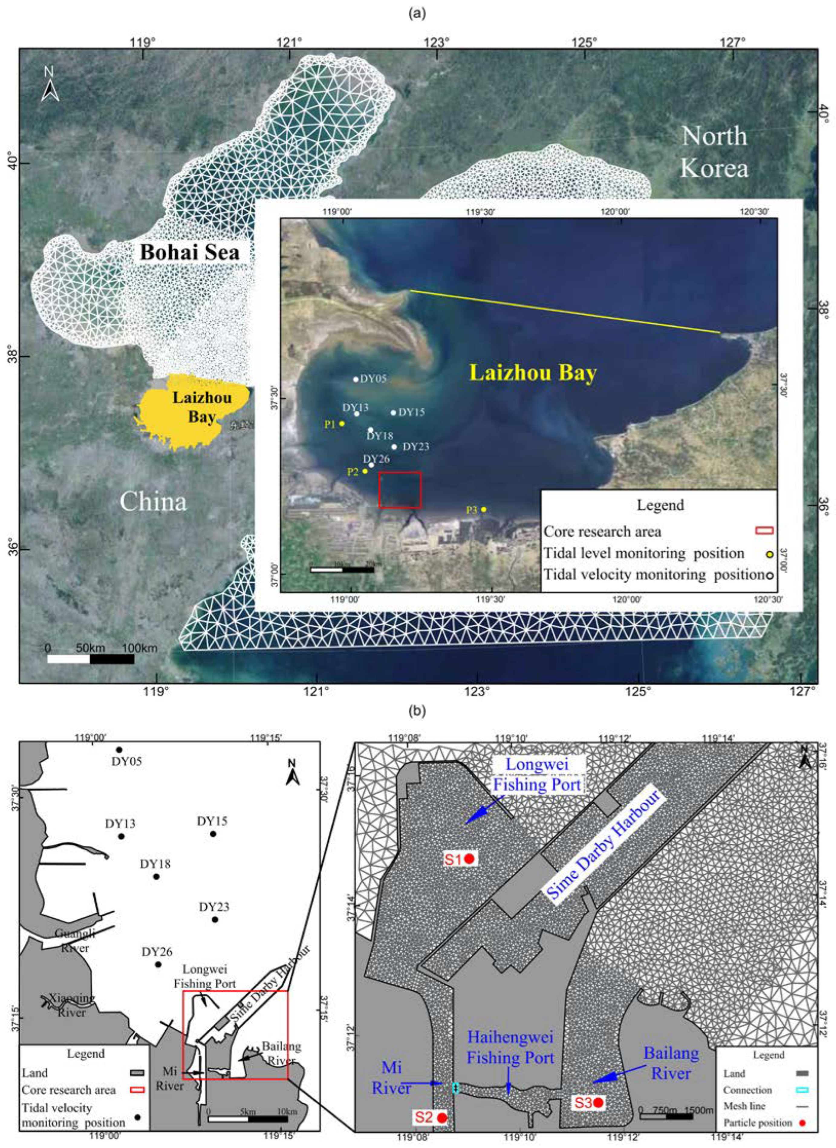
2.1. Study Area

Laizhou Bay is the largest sea bay in Shandong Province, China, which starts from the mouth of the Yellow River (37°39′ N, 119°16′ E) in the west and ends at Qimu Island in the east (37°41′10″ N, 120°13′10″ E) (Figure 1a). The straight-line diameter of the bay from west to east is about 100 km, the coastline is 319.6 km long, and the bay area is 6966 km². Laizhou Bay has a smooth seabed morphology with an average depth of <10 m. The deepest point is in the western part of the bay, at a depth of 18 m. The bay is important for the local marine industry and economy. The southwestern part of Laizhou Bay is mostly a port area, which is affected by many human development activities.

In the southwest of Laizhou Bay, Sime Darby Harbor is encompassed by two 17.3 km long sand-retaining embankments built in 2010. These embankments are perpendicular to the shoreline, and the Mi River (Mi River estuary: 37°09′30″ N–37°13′00″ N, 119°08′05″ E–119°08′30″ E) and the Bailang River (Bailang River estuary: 37°10′30″ N–37°13′00″ N, 119°10′30″ E–119°12′00″ E) are located on the two sides of the embankments, or Sime Darby Harbor (Figure 1b).

In the near shore area, a core research area (as shown in Figure 1b) was defined in this study to investigate the water transport capacity inside and outside of the Sime Darby Harbor. The study area is approximately 100 km² in size and situated within the coordinates of 37°11′22.56″ N to 37°17′02.79″ N and 119°06′52.87″ E to 119°16′02.42″ E. It covers Longwei Fishing Port, Mi River, Bailang River, Haihengwei Fishing Port and most of Sime Darby Harbor.

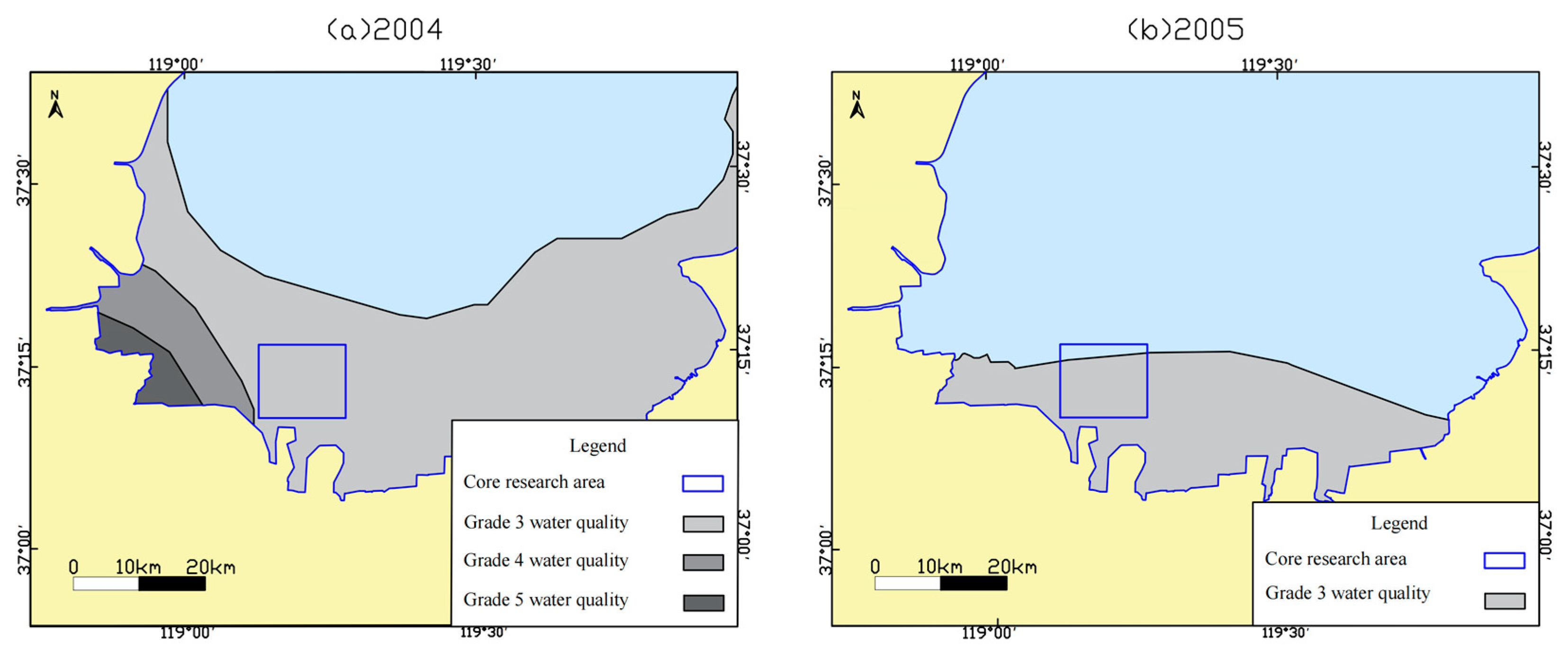
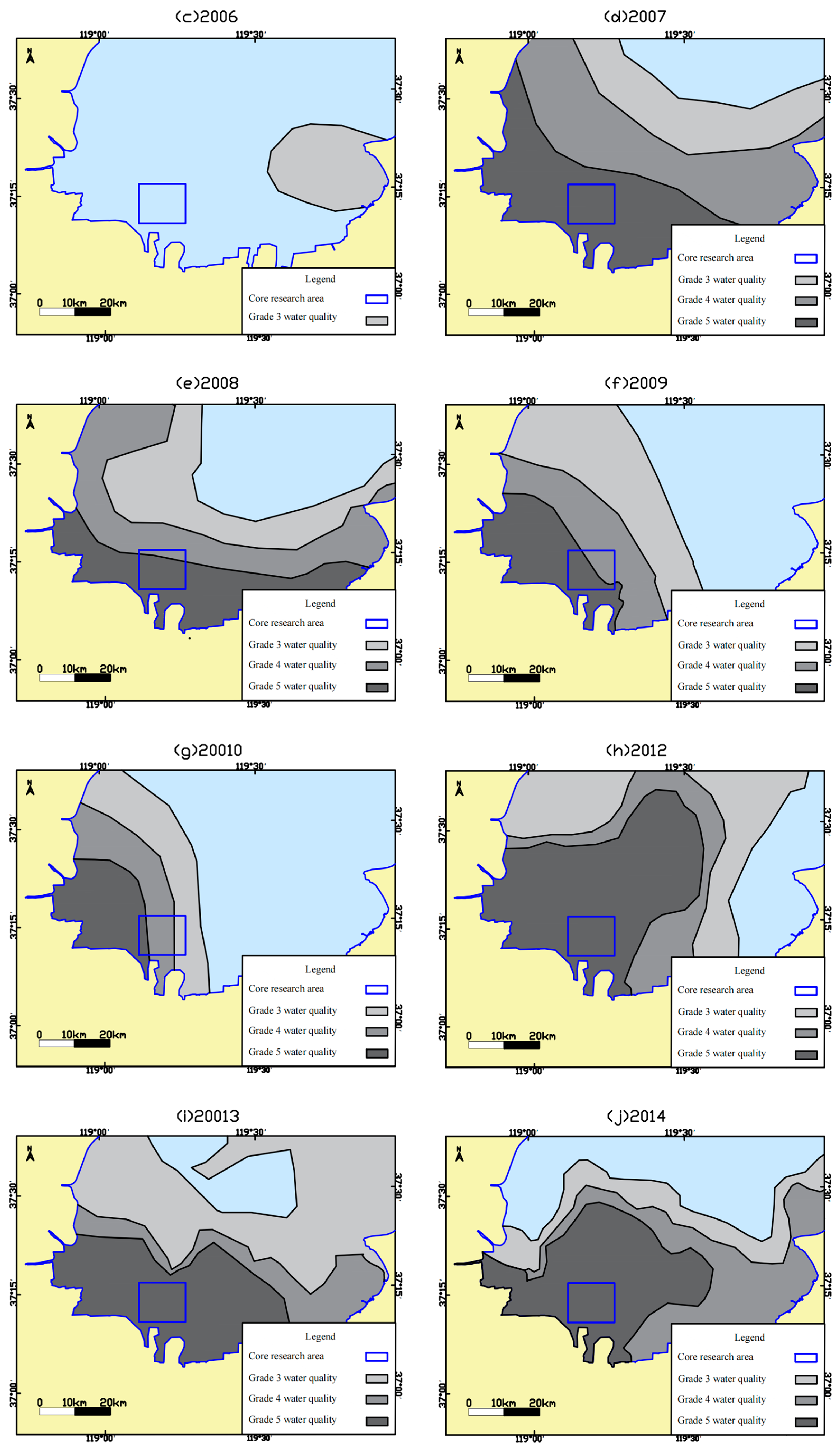
2.2. Water Quality Issue

Laizhou Bay is a typical semi-enclosed bay with poor hydrodynamic conditions and low water exchange and self-purification capabilities [22]. In China, the National Sea Water Quality Standard [23] requires port waters to reach Grade 4, and Grade 5 is deemed to be unqualified (accessed on Ministry of Ecology and Environment of the People’s Republic of China). Grade 3 is required for industrial water use and coastal scenic tourism. However, as per the Marine Environmental Status Bulletin of Shandong Province, China, the results of 180 water quality monitoring sites show that the area with Grade 5 water quality in the Laizhou Bay increased sharply from 2010 to 2012 (Figure 2), from 312.1 km² to 1621.1 km² (

Table 1. The water surface areas with various water quality grades in the Laizhou Bay in 2004–2014. Data source: Marine Environment Bulletin of Shandong Province, China.

Year	Water Area (km2) with Water Quality of
	Grade 5	Grade 4	Grade 3
2014	1116.5	2523.9	3572.9
2013	1112.9	1852.3	4989.5
2012	1621.1	2408.6	3602.9
2011	—	—	—
2010	312.1	766.3	1423.4
2009	336.1	1053.7	2351.4
2008	720.1	2166.8	3469.1
2007	1132.1	2942.2	4179.9
2006	—	—	620.1
2005	—	—	694.5
2004	100.0	186.2	2860.8

). After 2012, although the area decreased, it still exceeded 1000 km². Compared with previous years, in 2012, 2013, and 2014, the area with Grade 5 water quality was predominantly concentrated in specific regions in southwestern Laizhou Bay, completely covering the core research area (Figure 2). Overall, the water quality in southwestern Laizhou Bay has severely deteriorated since 2010 after the completion of Sime Darby Harbor.

3. Numerical Model

3.1. Model Description

Mike 21 Flow Model (FM) was used in this study for hydrodynamic modeling and Lagrangian particle tracking. The whole research area was discretized and decomposed using the mesh method (accessed on MIKE Powered by DHI), which included triangular and quadrilateral meshes to better adapt to the complexity of the coastline and different scenarios (Figure 1b). The boundary conditions of the model included wind friction at the sea surface, friction at the seabed, Coriolis forces, and water flowing at point pollution sources. Tidal components (M₂, S₂, O₁ and K₁) were determined as constants based on long-term modeling results of tidal elevation, which were obtained from the East China Sea Dynamic Model of the North Sea Forecast Center and the long-term tidal level in the vicinity.

The open boundary line of the tidal field was established as the connecting line between Rizhao City, China, and Busan City, South Korea, with a total modeling area of about 360,000 km². The modeling area was between 35° and 41° N and 117° and 127° E, and was about 750 km wide from east to west and 650 km long from north to south, covering the entirety of Laizhou Bay. This area was divided into subareas with grids of different resolution, and local refinement was carried out in the study area in the southwest of Laizhou Bay. There were 34,952 nodes and 66,439 elements for the horizontal mesh generation in the entire modeling area (Figure 1a), and the maximum size of the element was about 10–20 km near open boundary, with element sizes decreasing closer to the core research area. Within the core research area, the minimum element size was about 60 m (Figure 1b).

The model simulation covered the time period from 11 July 2011 to 11 August 2011, with a time step of one hour. The bed resistance type was the Manning number with a constant value of 32 m^1/3/s in the research area, and the Smagorinsky formulation was used for eddy viscosity with a constant value of 0.28. In addition, the long-term transport effects of wind on matter are relatively insignificant in the tidally controlled Laizhou Bay; thus, the influence of wind forcing was not considered in this numerical simulation.

The water depth data were obtained from Chart No. 12510 and 12570 of the Navigation Guarantee Department of Chinese Navy Headquarters, derived from the Chinese official water depth data for the public. Tidal level data were extracted from DHI C-MAP provided by Mike 21. The coastline of Laizhou Bay was obtained from the Landsat 8 image data in January 2012 with a spatial resolution of 15 m. The image was preliminarily processed via visual image interpretation, and the natural shoreline was determined via a spot survey.

3.2. Control Equations

The model built in Mike 21 included the mass conservation equation and the momentum equation [24].

(1)

Continuity equation:

$$\frac{\partial \zeta }{\partial t}+\frac{\partial }{\partial x}\left(hu\right)+\frac{\partial }{\partial y}\left(hv\right)=0$$

(1)

In this equation, $x$ and $y$ are right-handed Cartesian coordinates, $u$ and $v$ are the velocity components in the $x$ and $y$ directions, respectively, $t$ is the simulated time, $\zeta$ is the mean water level, and $h$ is the still water depth.

(2)

Momentum equation:

$$\frac{\partial u}{\partial t}+u\frac{\partial u}{\partial x}+v\frac{\partial u}{\partial y}-\frac{\partial }{\partial x}\left({\epsilon }_x\frac{\partial u}{\partial x}\right)-\frac{\partial }{\partial y}\left({\epsilon }_x\frac{\partial u}{\partial y}\right)-fv+\frac{gu\sqrt{u^2+v^2}}{C_Z^{2}H}=-\mathrm{g}\frac{\partial \zeta }{\partial x}$$

(2)

$$\frac{\partial v}{\partial t}+u\frac{\partial v}{\partial x}+v\frac{\partial v}{\partial y}-\frac{\partial }{\partial x}\left({\epsilon }_x\frac{\partial v}{\partial x}\right)-\frac{\partial }{\partial y}\left({\epsilon }_y\frac{\partial v}{\partial y}\right)+fu+\frac{gv\sqrt{u^2+v^2}}{C_Z^{2}H}=-g\frac{\partial \zeta }{\partial y}$$

In Equation (2), g is the gravitational acceleration, ${\epsilon }_x$ and ${\epsilon }_y$ are the horizontal eddy viscosity coefficients in the $x$ and $y$ directions, respectively, and $H$ is the total water depth measured from the water level to the bottom of the considered water body, which can be expressed as:

$$H=h+\zeta$$

(3)

In addition, $f$ is the Coriolis force, which can be expressed as:

$$f=2\omega sin\phi$$

(4)

where $\omega$ is the angular speed of the earth and $\phi$ is the latitude of the sea area. $C_Z$ is the Chezy coefficient, $n$ is the Manning coefficient, and their relationship can be expressed as [25]:

$$C_Z=n{H}^{\frac{1}{6}}$$

(5)

3.3. Initial and Boundary Conditions

The driving factors for the water level change at the open boundary can be divided into tidal and non-tidal factors. Laizhou Bay is adjacent to the boundary between the Yellow Sea and the Bohai Sea, and these influencing factors should be comprehensively considered. Thus, the definite conditions were calculated as follows [26]:

(1)

Initial conditions:

$$\left\{\begin{array}{c}\zeta \left(x,y,t\right){|}_{t=t_0}=\zeta \left(x,y,t_0\right)=0\\ u\left(x,y,t\right){|}_{t=t_0}=v\left(x,y,t\right){|}_{t=t_0}=0\end{array}\right.$$

(6)

(2)

Boundary conditions:

The normal velocity of the fixed boundary was taken as:

$$\overrightarrow{V}\cdot \overrightarrow{n}=0$$

(7)

where $\overrightarrow{V}$ is the velocity of the rigid surface and $\overrightarrow{n}$ is the unit normal vector of the surface pointing into the fluid at a given location [27].

Open boundary treatment was adopted in the tidal flat area, and the water boundary was controlled by the tide forecast [26]:

$$\zeta =A_0+\sum \sum _{i=1}^k{H}_i{F}_i\cos \left[{\sigma }_{it}t-{\left(v_0+u\right)}_i+g_i\right]$$

(8)

where $A_0$ is the average sea level and $H_i$ and $g_i$ are harmonic constants of certain tidal components, expressing the amplitude and epoch of partial tides, respectively. In Equation (8), ${\left(v_0+u\right)}_i$ is an astronomical argument with time-dependent factors, $F_i$ is the nodal amplitude factor, and $k$ is the number of tidal components.

3.4. Modeling Scenarios

There were two modeling scenarios in this study, i.e., before and after connecting the two rivers (Mi River and Bailang River) on the two sides of the sand retaining embankments of Sime Darby Harbor. The focus was to examine the difference in hydrodynamics and particle transport between the two scenarios, so the simulation needed to control variables. The water depth at the connection was the only variable in different scenarios to avoid other factors being affected. Compared to the water depth before connecting the rivers, the adjusted depth is validated based on the average in the vicinity of the connection, which has stabilized with the prolonged sedimentation and erosion.

In each scenario, both the tidal current and the residual current were simulated because the flow in the sea bay is a comprehensive cumulative result of the periodic tidal current and the aperiodic residual current. The tidal current is a relatively stable water movement driven by astronomical tides and its periodicity indirectly affects water exchange [28]. Tidal current and coastal topography are the main factors affecting residual current, exhibiting non-periodicity [29]. Residual current has a direct impact on the transport of sediments, suspended solids, and soluble substances in oceans, and thus affects the water quality in the sea area [29,30].

There are two calculation methods for tidal and residual currents, which were both used in this study. (1) Tidal current can be calculated using two or three-dimensional equations of tidal wave motion, and then Eulerian residual current can be obtained [31]. Meanwhile, the (2) Lagrangian residual current can be calculated based on the non-linear, two or three-dimensional Lagrangian average or mean flow theory [32].

In addition to tidal and residual currents, particle tracking is also an important means to study the exchange capacity of water bodies based on the Lagrangian tidal residual current.

At each position in S1, S2, and S3, 100 particles were released at a depth of 0.5 m underwater at the initial time, and the number of particles remained unchanged thereafter (S1, S2, and S3 in Figure 1b, located at the Longwei Fishing Port, Mi River estuary and Bailang River estuary). Every particle had a mass of 0 kg without decay or influence from wind in order to focus on the long-term transport in the tide-controlled Laizhou Bay. Their horizontal and vertical dispersion coefficients are 0.001 m²/s and 0 m²/s, respectively (commonly, the dispersion coefficient is difficult to measure directly; thus, it is often substituted with empirical values or calculated by means of scaled eddy viscosity formulation. In this study, empirical values were adopted to investigate particle movement in the horizontal direction). Particles were tracked in terms of transport distance based on hydrodynamics in one month for the two modeling scenarios.

4. Results and Discussion

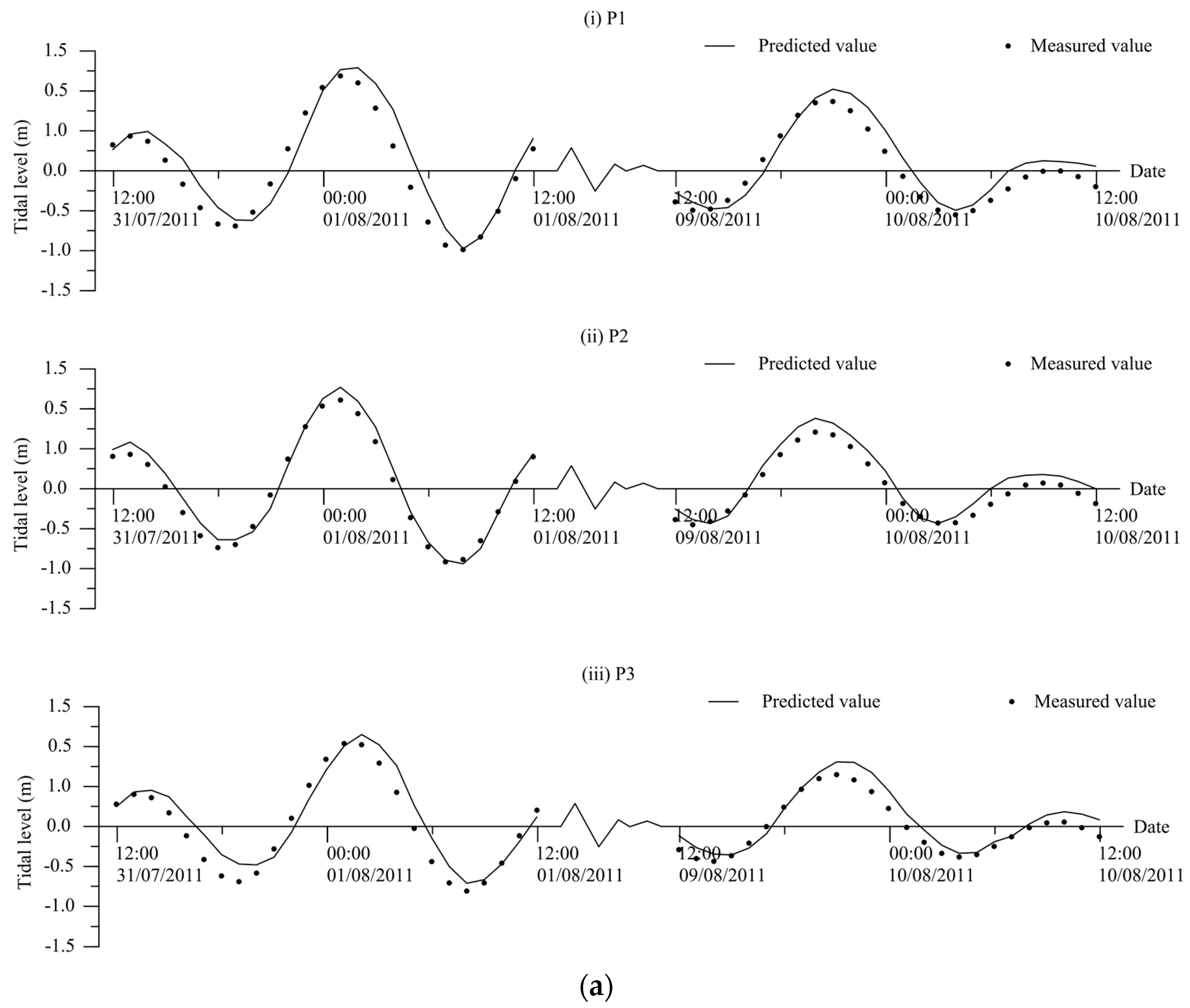
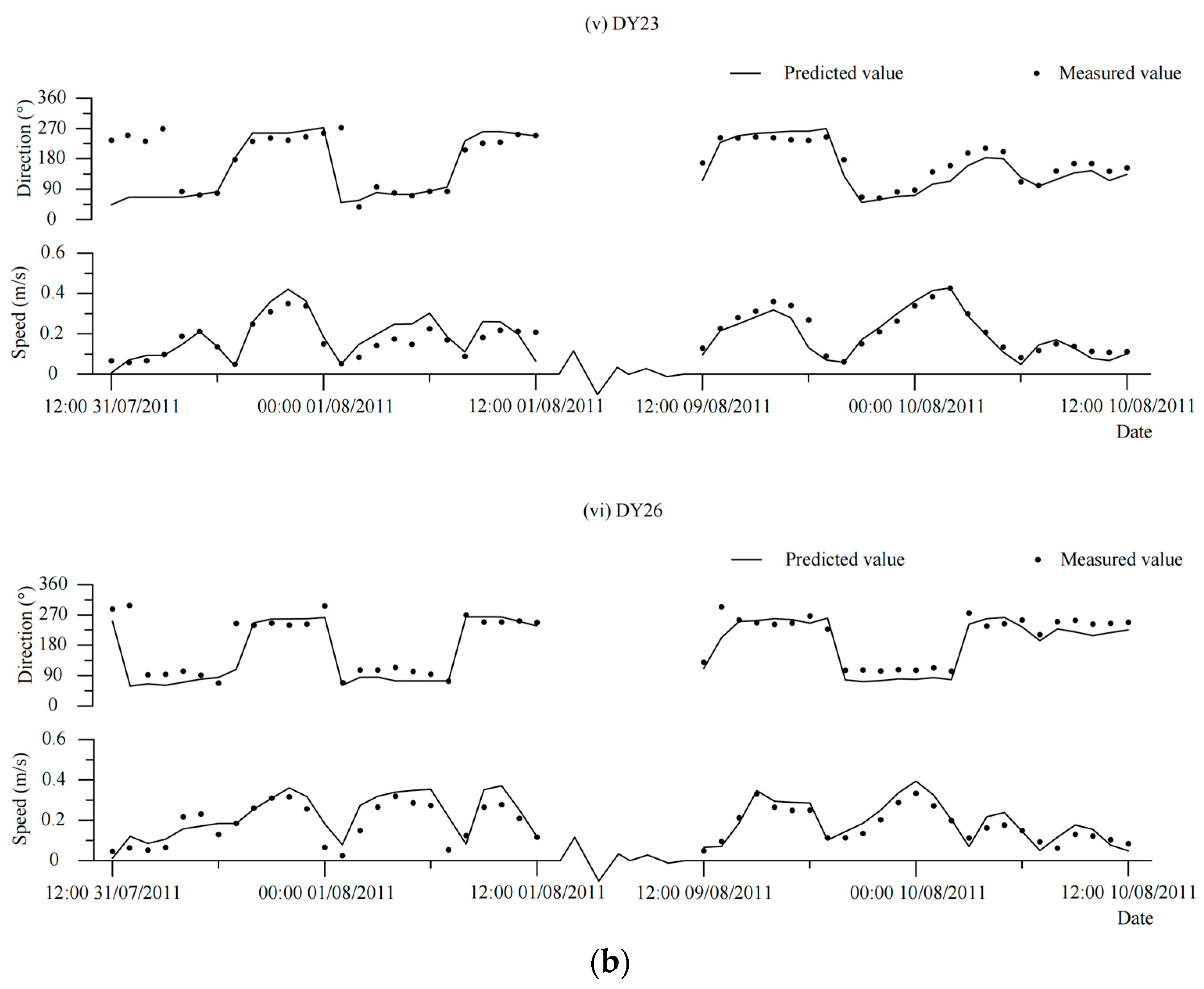
4.1. Model Validation

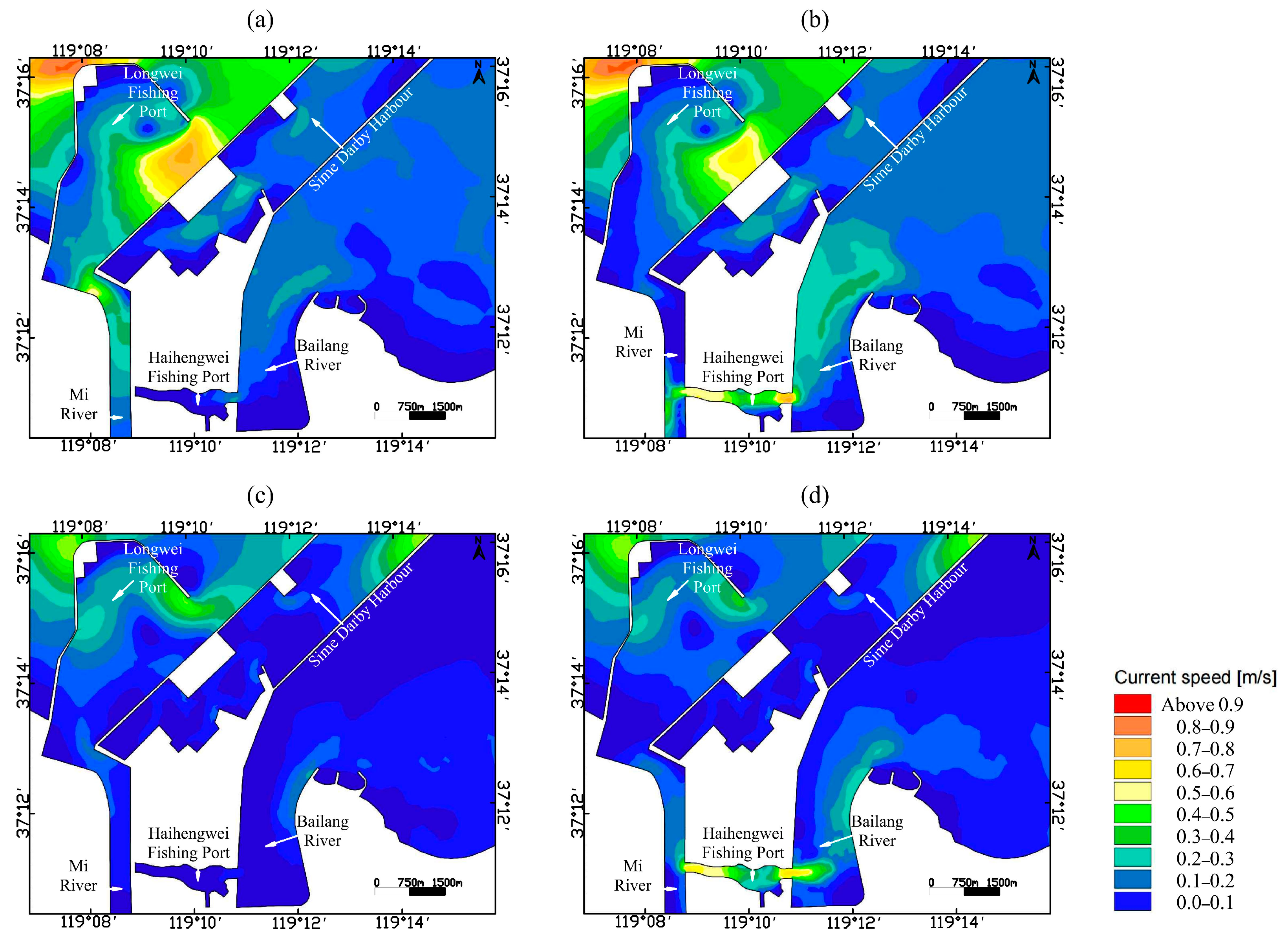
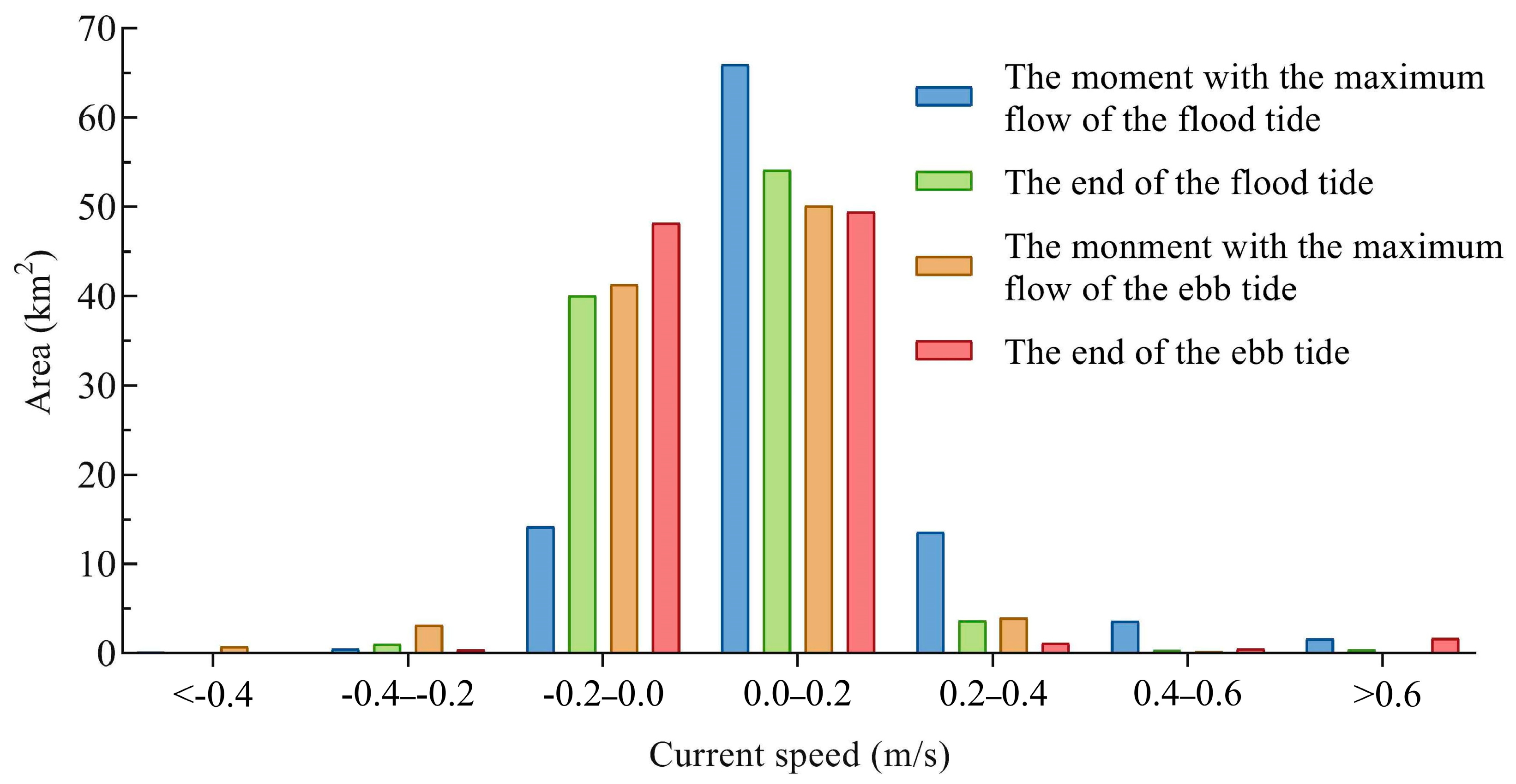
The model was validated with the field data monitored by the Beihai Ocean Prediction Center and the State Oceanic Administration of China. In the early stage of the simulation, the model is in a transitional phase, and there exists some discrepancy between the simulated and the measured data, which gradually diminishes thereafter (Figure 3). After the transitional phase, the averages of the root mean square error (RMSE) for water level, tidal current and direction are 0.16 m, 0.06 m/s and 37.99°, respectively, between the simulated and measured data. Meanwhile, the average square of the Pearson’s correlation coefficient (R²) for these variables is 0.83 (

Table 2. Validation results of water level, current speed and direction between the measured and predicted data.

Tidal Level
Location	Tidal Periodicity	RMS (m)		RMSE (m)	R2
		Measured Value	Predicted Value
P1	Spring tide	0.65	0.67	0.23	0.91
	Neap tide	0.45	0.49	0.15	0.93
P2	Spring tide	0.62	0.66	0.12	0.98
	Neap tide	0.37	0.42	0.12	0.98
P3	Spring tide	0.57	0.56	0.19	0.92
	Neap tide	0.34	0.38	0.13	0.95
Average		0.50	0.53	0.16	0.95
Current Speed
Location	Tidal Periodicity	RMS (m/s)		RMSE (m/s)	R2
		Measured Value	Predicted Value
DY05	Spring tide	0.24	0.21	0.06	0.80
	Neap tide	0.24	0.21	0.04	0.94
DY13	Spring tide	0.21	0.19	0.06	0.76
	Neap tide	0.19	0.16	0.05	0.82
DY15	Spring tide	0.27	0.26	0.07	0.74
	Neap tide	0.29	0.29	0.04	0.93
DY18	Spring tide	0.34	0.37	0.08	0.82
	Neap tide	0.19	0.19	0.03	0.86
DY23	Spring tide	0.31	0.34	0.08	0.81
	Neap tide	0.24	0.23	0.04	0.90
DY26	Spring tide	0.34	0.37	0.09	0.68
	Neap tide	0.19	0.22	0.04	0.90
Average		0.25	0.25	0.06	0.83
Current Direction
Location	Tidal Periodicity	RMS (°)		RMSE (°)	R2
		Measured Value	Predicted Value
DY05	Spring tide	175.31	192.50	55.56	0.70
	Neap tide	215.22	202.97	28.41	0.90
DY13	Spring tide	171.04	164.44	49.59	0.71
	Neap tide	208.17	194.36	31.24	0.91
DY15	Spring tide	205.42	227.88	62.40	0.69
	Neap tide	208.54	198.95	18.30	0.91
DY18	Spring tide	198.65	203.11	35.21	0.88
	Neap tide	189.42	183.28	29.00	0.97
DY23	Spring tide	220.04	245.38	57.01	0.76
	Neap tide	179.02	170.82	26.43	0.89
DY26	Spring tide	193.66	204.48	32.45	0.91
	Neap tide	215.38	201.52	30.28	0.88
Average		198.32	199.14	37.99	0.84

), indicating that the model reasonably represents the tidal characteristics.

4.2. Tidal Current

Tidal currents can reveal the strength of water exchange capacity [33,34], so the tides are simulated before and after connecting the Mi River and the Bailing River. During both the flood and ebb phases, the variation of tidal current speed is non-uniform in the core research area (Figure 4, Figure 5 and Figure 6).

At the moment of maximum flow of the flood phase (Figure 4a,b), the increase in tidal current speed is the most pronounced throughout the entire tidal cycle, with a notable rise observed within approximately 85 km² in the core research area of 100 km². The tidal current speed shows a predominant increase of 0.0–0.2 m/s, encompassing an area of roughly 66 km². Additionally, the areas exhibiting an increase of 0.2–0.4 m/s, 0.4–0.6 m/s, and above 0.6 m/s account for 14 km², 4 km², and 2 km², respectively, which are also significantly larger compared to other times (Figure 6). The maximum increase is observed to be 1.0 m/s at the location of 37°11′55.33″ N and 119°10′53.20″ E, which is on the eastern side of Haihengwei Fishing Port.

At the end of the flood phase (Figure 4c,d), the area experiencing an increase in current speed is 59 km² (out of 100 km²), which is 18 km² more than the area where the current speed decreases in the core research area. The variations in current speed are primarily concentrated within the ranges of −0.2–0.0 m/s and 0.0–0.2 m/s, covering respective areas of 40 km² and 54 km². Furthermore, there is an additional area of 4 km² where the current speed increases by 0.2–0.4 m/s, primarily concentrated on both the eastern and western sides of Haihengwei Fishing Port (Figure 6).

At the moment of maximum flow of the ebb phase (Figure 5a,b), the pattern of current speed variation resembles the end of the flood phase. The area experiencing an increase in current speed of 0.0–0.2 m/s is 50 km², while the area experiencing a decrease in current speed of 0.0–0.2 m/s is 41 km². Additionally, the area where the current speed increases by 0.2–0.4 m/s covers 4 km², which is also primarily located within Haihengwei Fishing Port and to its east, near Bailang River. There is an area of 3 km² where the current speed decreases by 0.2–0.4 m/s, which is concentrated at the Mi River estuary (Figure 6).

At the end of the ebb phase (Figure 5c,d), the area (51 km²) experiencing an increase in current speed is slightly larger than that (49 km²) experiencing a decrease. Among these, the area where the current speed increases by 0.0–0.2 m/s covers 49 km², while the area where the current speed decreases by 0.0–0.2 m/s covers 48 km² (Figure 6). The most notable current speed changes occur prominently at the connection of the Mi River and Bailang River, where the current speed experiences by a maximum increase of 0.6 m/s.

In short, regardless of a flood phase or ebb phase, the water areas experiencing velocity increases exceed 53% of the core research area of 100 km² (Figure 6). Tidal influence can dilute nutrient concentrations [33], and also can displace dissolved and suspended matter near river mouths [34]. The locations where Haihengwei Fishing Port intersects with both rivers, where tidal currents increase significantly, are highly likely to accelerate water exchange near the coast and enhance the self-purification capacity of the water body.

4.3. Eulerian Residual Current

After the connection of the two rivers, the most obvious changes in the residual current are mainly concentrated at the junctions of the Mi River, Haihengwei Fishing Port, and Bailang River (Figure 7). Upon connecting the two rivers through the Haihengwei Fishing Port, there is a substantial increase in residual currents within the port. In the Haihengwei Port, the predominant current direction is from the Mi River to the Bailang River, and the significant increases from almost 0 to 0.11 m/s occurred at the confluences of Haihengwei Fishing Port with the two rivers. The maximum variation of the residual velocity at the mouths of the Mi River and Bailang River increased to about 0.16 m/s and 0.20 m/s, respectively, and the previous velocities at these locations were very weak, almost negligible.

Furthermore, at both extremities of the Haihengwei Fishing Port, four eddies of varying sizes form at the Mi River estuary and Bailang River estuary after the river connection (Figure 7), which is primarily caused by residual flows within the Haihengwei Fishing Port from west to east. The most prominent eddy is located on the northeast side of the Haihengwei Fishing Port, with the center of the eddy estimated to be at approximately 37°11′30.34″ N and 119°11′23.48″ E (Figure 7). There is no obvious change in the clockwise vortex in the Longwei Fishing Port, and the center of the vortex is still at approximately 37°15′00.11″ N and 119°09′15.53″ E.

However, the elliptical vortex in the northeastern Longwei Fishing Port, with a consistent center at 37°15′41.16″ N and 119°10′41.51″ E, experiences a decrease in the average residual velocity from 0.10 m/s to 0.09 m/s. The residual current field in Sime Darby Harbour also experiences no significant change after the river connection, with an average change of only 0.01 m/s.

The simulation results of the Eulerian residual current indicate an obvious increase in the vicinity of the connection. Comparing the pre- and post-connection periods, the maximum increase in Eulerian residual current is 0.17 m/s and the maximum decrease is 0.15 m/s. The increase in Euler residual current can enhance the mass transfer capacity and reduce pollutant concentrations [35]. There is a positive correlation between the magnitude of residual flow and water exchange capacity focusing on Bohai Sea [36]. This further reveals that the water quality can be improved in the nearshore areas after the connection of the two rivers through the Haihengwei Fishing Port.

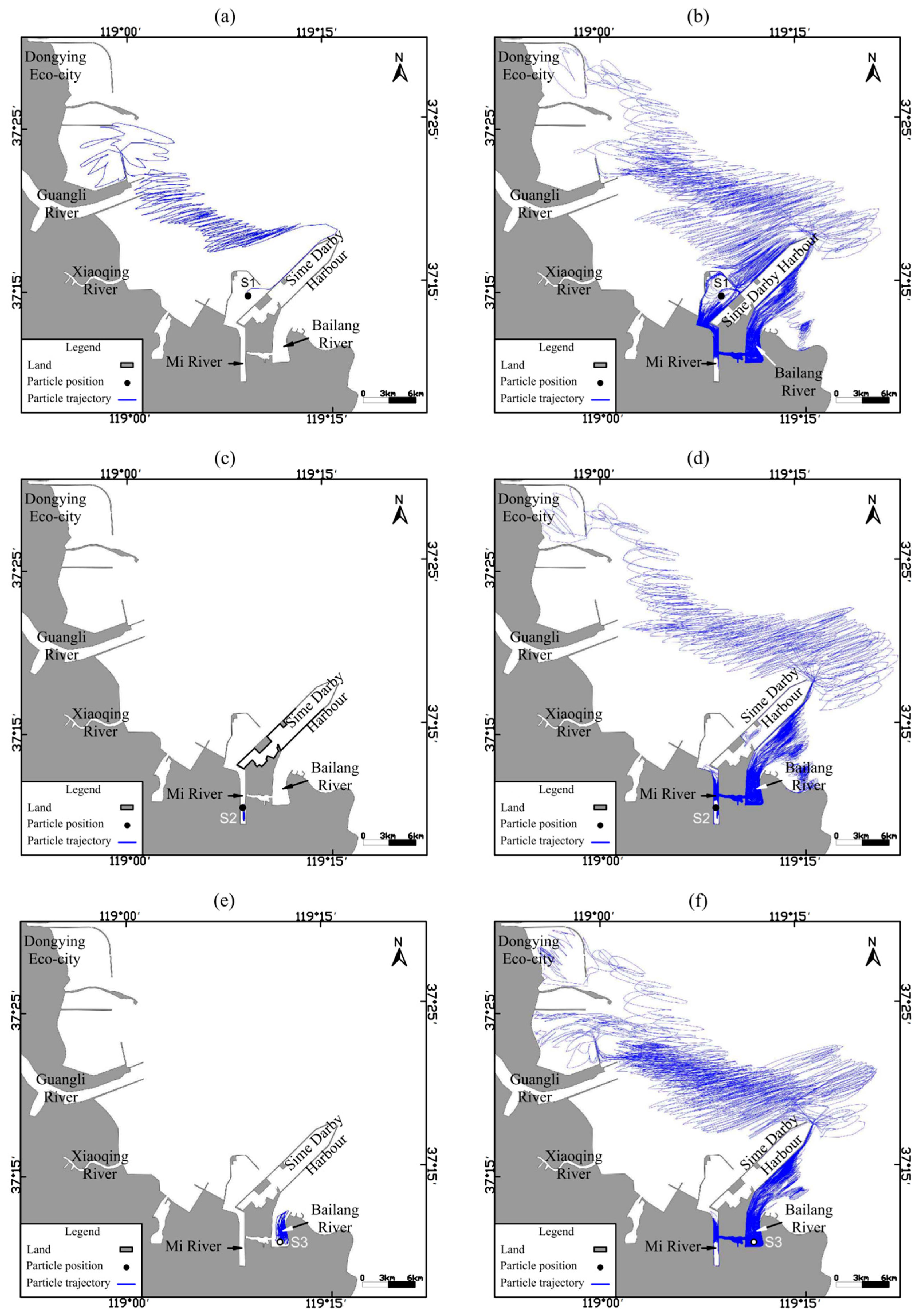
4.4. Lagrangian Particle Tracking

The results of tracking particles over a month indicate that the transport distance has increased substantially after the connection between the two rivers (

Table 3. The net transport distance of particles S1, 2 and 3 at different positions before and after the connection of the two rivers.

Particle	Net Transport Distance (km)		Increase
	Before Connection	After Connection	(km)	(%)
S1	24.9	33.4	8.5	34.2
S2	1.8	41.8	39.9	2.2 × 103
S3	3.7	42.1	38.4	1.0 × 103

). Point S1 is in the Longwei Fishing Port, where the particle moves to the sea along the west side of the embankment before the connection (Figure 8a). After the connection, the movement trajectory of the particles covers the Longwei Fishing Port, the Mi River estuary, the Haihengwei Fishing Port, and the Bailang River (Figure 8b). The net transport distance increased from 24.9 km to 33.4 km in a month, i.e., an increase of about 8.5 km.

When the particle at point S2 starts moving in the Mi estuary, its trajectory is characterized by short-distance reciprocation before the connection, with a maximum net transport distance of only 1.8 km (Figure 8c). After the connection, the particle trajectory for a month first enters the Haihengwei Fishing Port and then enters the sea from the Bailang River, with a maximum transport distance of 41.8 km. The net transport distance of the particle is about 39.9 km and the trajectory reaches Dongying eco-city (Figure 8d).

Similarly, the particle released at point S3 lingers in the Bailang estuary for a long time before the connection (Figure 8e). After the connection, the particle movement path becomes complicated. It flows with the water through the Haihengwei Fishing Port and the Mi River estuary, and finally moves to Dongying eco-city (Figure 8f). The net transportation distance within one month increases from 3.7 km before the connection to 42.1 km after the connection.

In summary, the net transport distance of the released particles increases by a maximum of 2.2 × 10³% (Table 3). Similarly, particles can be regarded as pollutants, and thus water quality changes can also be indirectly reflected through particle movement [18]. The longer the particles stay in a certain location, the weaker the water exchange at that location [37]. The results again reveal that after connecting the Mi River and the Bailang River, particles are highly likely to be transported more rapidly along both sides of the embankment to Laizhou Bay, promoting water exchange and improving water quality in the Bay.

5. Conclusions

In the southwest of Laizhou Bay, two embankments were built for Sime Darby Harbor, weakening the water exchange and deteriorating the water quality in the bay. This study proposed connecting the two rivers on both sides of the embankments to improve hydrodynamics and thus water quality. The tidal current, Euler residual current, and Lagrangian particle tracking were numerically examined before and after the connection through a well-validated Mike 21 FM model.

The results show that, after the connection, more than 53% of the core research area (53 km²) displays an increase in tidal current velocity, and it is primarily concentrated in the internal and nearby coastal areas surrounding the connection (Haihengwei Fishing Port). In particular, the largest increase in tidal current speed reaches 0.6 m/s in the Bailang River near the Haihengwei Fishing Port. There are also increases in Eulerian residual currents in the Mi River, the Bailang River, and within the Haihengwei Fishing Port after the connection. Notably, the largest increase in residual currents occurs in the Bailang River and is approximately 0.17 m/s, and the vortex is more pronounced at the Bailang River estuary. The particles released at the estuaries are also more easily transported into the sea bay, and the maximum net transport distance increases by 39.9 km in a month. These results demonstrate that the capacity of water exchange can be enhanced after the river connection, and thereby the long-term transport of the water body is improved in the southwest of Laizhou Bay.

This study provides an effective measure to improve poor hydrodynamics and water quality induced by the construction of large coastal structures such as embankments or dikes and supports the sustainable development of sea bays.

References

1. Kateb, A.E.; Stalder, C.; Rüggeberg, A.; Neururer, C.; Spangenberg, J.E.; Spezzaferri, S. Impact of industrial phosphate waste discharge on the marine environment in the Gulf of Gabes (Tunisia). PLoS ONE 2018, 13, 0197731. [Google Scholar] [CrossRef] [PubMed]
2. Fasano, E.; Arnese, A.; Esposito, F.; Albano, L.; Masucci, A.; Capelli, C.; Cirillo, T.; Nardone, A. Evaluation of the impact of anthropogenic activities on arsenic, cadmium, chromium, mercury, lead, and polycyclic aromatic hydrocarbon levels in seafood from the Gulf of Naples, Italy. J. Environ. Sci. Health 2018, 53, 786–792. [Google Scholar] [CrossRef] [PubMed]
3. Rahman, M.A.; Dawes, L.; Donehue, P.; Rahman, M.R. Cross-temporal analysis of disaster vulnerability of the southwest coastal communities in Bangladesh. Reg. Environ. Chang. 2021, 21, 67. [Google Scholar] [CrossRef]
4. Xu, T.; You, X. Effects of large-scale embankments on the hydrodynamics and salinity in the Oujiang River Estuary, China. J. Mar. Sci. Technol. 2017, 22, 71–84. [Google Scholar] [CrossRef]
5. Ebrahimi-sirizi, Z.; Riyahi-bakhtiyari, A. Petroleum pollution in mangrove forests sediments from Qeshm Island and Khamir Port—Persian Gulf, Iran. J. Environ. Monit. Assess. 2013, 185, 4019–4032. [Google Scholar] [CrossRef] [PubMed]
6. Gao, F.; Zhang, C.; Jin, R.; Chen, S. The Development of Offshore Artificial Island Construction and Application of Key Hydrodynamic Technologies in China—Take Haihua Island Project as an Example. IOP Conf. Ser. Earth Environ. Sci. 2020, 580, 012093. [Google Scholar] [CrossRef]
7. Guo, L.; Zhu, C.; Xu, F.; Xie, W.; Van Der Wegen, M.; Townend, I.; Wang, Z.B.; He, Q. Reclamation of tidal flats within tidal basins alters centennial morphodynamic adaptation to sea-level rise. J. Geophys. Res. Earth Surf. 2022, 127, 249857249. [Google Scholar] [CrossRef]
8. Chi, W.; Zhang, X.; Zhang, W.; Bao, X.; Liu, Y.; Xiong, C.; Liu, J.; Zhang, Y. Impact of tidally induced residual circulations on chemical oxygen demand (COD) distribution in Laizhou Bay, China. Mar. Pollut. Bull. 2020, 151, 110811.1–110811.13. [Google Scholar] [CrossRef]
9. Gao, X.; Zhuang, W.; Chen, C.; Zhang, Y. Sediment Quality of the SW Coastal Laizhou Bay, Bohai Sea, China: A Comprehensive Assessment Based on the Analysis of Heavy Metals. PLoS ONE 2015, 10, e0122190. [Google Scholar] [CrossRef]
10. Hu, K.; Zhang, W.; Wang, X. Simulation of the Impact of Breakwaters on Hydrodynamic Environment in Laizhou Bay, China. J. Ocean Univ. China 2022, 21, 1557–1564. [Google Scholar] [CrossRef]
11. Vona, I.; Gray, M.W.; Nardin, W. The Impact of Submerged Breakwaters on Sediment Distribution along Marsh Boundaries. Water 2020, 12, 1016. [Google Scholar] [CrossRef]
12. Zhang, H.; Shen, Y.; Tang, J. Numerical investigation of successive land reclamation effects on hydrodynamics and water quality in Bohai Bay. Ocean Eng. 2023, 268, 113483. [Google Scholar] [CrossRef]
13. Yang, Y.; Liang, S.; Li, K.; Liu, Y.; Lv, H.; Li, Y.; Wang, X. Administrative responsibility and land-sea synergistic regulating indicators for nutrient pollution: Linking terrigenous emission to water quality target in Laizhou Bay, China. Ecol. Indic. 2022, 13, 108884. [Google Scholar] [CrossRef]
14. Komyakova, V.; Jaffrés, J.B.D.; Strain, E.M.A.; Cullen-Knox, C.; Fudge, M.; Langhamer, O.; Bender, A.; Yaakub, S.M.; Wilson, E.; Allan, B.J.M.; et al. Conceptualisation of multiple impacts interacting in the marine environment using marine infrastructure as an example. Sci. Total Environ. 2022, 830, 154748. [Google Scholar] [CrossRef] [PubMed]
15. Ranjbar, M.H.; Jandaghi, A.M.; Nazarali, M. A modeling study of the impact of increasing water exchange rate on water quality of a semi-enclosed bay. Ecol. Eng. 2019, 136, 177–184. [Google Scholar] [CrossRef]
16. Kazempour, Z.; Danesh, Y.M. Spatiotemporal dynamics of chlorophyll-a in the Gorgan Bay and Miankaleh Peninsula biosphere reserve: Call for action. Remote Sens. Appl. Soc. Environ. 2023, 30, 100946. [Google Scholar] [CrossRef]
17. Serrano, D.; Flores-Verdugo, F.; Ramírez-Félix, E.; Kovacs, J.M.; Flores-de-Santiago, F. Modeling tidal hydrodynamic changes induced by the opening of an artificial inlet within a subtropical mangrove dominated estuary. Wetl. Ecol. Manag. 2020, 28, 103–118. [Google Scholar] [CrossRef]
18. Tao, B.; Xu, J.; Zhang, M.; Chun-Ming, C. Seawater exchange rates for harbors based on the use of Mike 21 coupled with transport and particle tracking models. J. Coast. Conserv. 2021, 25, 33. [Google Scholar]
19. Yan, J.; Chen, M.; Xu, L.; Liu, Q.; Shi, H.; He, N. Mike 21 Model Based Numerical Simulation of the Operation Optimization Scheme of Sedimentation Basin. Coatings 2022, 12, 478. [Google Scholar] [CrossRef]
20. Xuan, T.L.; Cong, P.N.; Quoc, T.V.; Tran, Q.Q.; Wright, D.P.; Anh, D.T. Multi-scale modelling for hydrodynamic and morphological changes of breakwater in coastal Mekong Delta in Vietnam. J. Coast. Conserv. 2022, 26, 18. [Google Scholar] [CrossRef]
21. Nguyen, P.; Gourbesville, P.; Audra, P.; Vo, N.D. Optimization of Channel Outlet in the Coastal Area—Application to Da Nang Bay, Viet Nam. Int. J. Environ. Sci. Dev. 2022, 13, 246–250. [Google Scholar] [CrossRef]
22. Lefebvre, C.; Rojas, I.J.; Lasserre, J.; Villette, S.; Morin, B. Stranded in the high tide line: Spatial and temporal variability of beached microplastics in a semi-enclosed embayment (Arcachon, France). Sci. Total Environ. 2021, 797, 149144. [Google Scholar] [CrossRef]
23. GB 3097-1997; Sea Water Quality Standard. Ministry of Ecology and Environment of the People’s Republic of China: Beijing, China, 1998.
24. Li, X.; Huang, M.; Wang, R. Numerical simulation of Donghu Lake hydrodynamics and water quality based on remote sensing and MIKE 21. ISPRS Int. J. Geo-Inf. 2020, 9, 94. [Google Scholar] [CrossRef]
25. Lambkin, D. A Review of the Bed Roughness Variable in MIKE 21 FLOW MODEL FM, Hydrodynamic (HD) and Sediment Transport (ST) Modules; English Heritage ALSF Project No. 5224; University of Southampton: Southampton, UK, 2010. [Google Scholar]
26. Wang, W.; Hu, Z.; Li, M.; Zhang, H. Assessment of Tidal Current Energy Resources in the Pearl River Estuary Using a Numerical Method. Water 2023, 15, 3990. [Google Scholar] [CrossRef]
27. Subramanian, R. Boundary Conditions in Fluid Mechanics; Clarkson University: Potsdam, NY, USA, 2019. [Google Scholar]
28. Wang, R.; Herdman, L.M.; Erikson, L.; Barnard, P.; Hummel, M.; Stacey, M.T. Interactions of estuarine shoreline infrastructure with multiscale sea level variability. J. Geophys. Res. Ocean 2017, 122, 9962–9979. [Google Scholar] [CrossRef]
29. Stashchuk, N.; Vlasenko, V.; Hosegood, P.; Nimmo-Smith, W.A. Tidally induced residual current over the Malin Sea continental slope. Cont. Shelf Res. 2017, 139, 21–34. [Google Scholar] [CrossRef]
30. Yang, Z.; Wang, T. Tidal residual eddies and their effect on water exchange in Puget Sound. Ocean Dyn. 2013, 63, 995–1009. [Google Scholar] [CrossRef]
31. Deng, F.; Jiang, W.; Valle-Levinson, A.; Feng, S. 3D Modal Solution for Tidally Induced Lagrangian Residual Velocity with Variations in Eddy Viscosity and Bathymetry in a Narrow Model Bay. J. Ocean Univ. China 2019, 18, 69–79. [Google Scholar] [CrossRef]
32. Mardani, N.; Khanarmuei, M.; Suara, K.; Brown, R.; McCallum, A.; Sidle, R.C. Lagrangian data assimilation for improving model estimates of velocity fields and residual currents in a tidal estuary. Appl. Sci. 2021, 11, 11006. [Google Scholar]
33. Cereja, R.; Brotas, V.; Nunes, S.; Rodrigues, M.; Cruz, J.P.; Brito, A.C. Tidal influence on water quality indicators in a temperate mesotidal estuary (Tagus Estuary, Portugal). Ecol. Indic. 2022, 136, 108715. [Google Scholar]
34. DiLorenzo, J.L.; Filadelfo, R.J.; Surak, C.R.; Litwack, H.S.; Gunawardana, V.K.; Najarian, T.O. Tidal variability in the water quality of an urbanized estuary. Estuaries 2004, 27, 851–860. [Google Scholar] [CrossRef]
35. Kong, X. Influence of inter-river water diversion on estuary pollution control: A case study of Liaodong Bay. Reg. Stud. Mar. Sci. 2024, 70, 103362. [Google Scholar] [CrossRef]
36. Wu, Z.; Zhou, C.; Wang, P.; Fei, Z. Responses of tidal dynamic and water exchange capacity to coastline change in the Bohai Sea, China. Front. Mar. Sci. 2023, 10, 2296–7745. [Google Scholar] [CrossRef]
37. Zhao, E.; Mu, L.; Qu, K.; Shi, B.; Ren, X.; Jiang, C. Numerical investigation of pollution transport and environmental improvement measures in a tidal bay based on a Lagrangian particle-tracking model. Water Sci. Eng. 2018, 11, 1674–2370. [Google Scholar] [CrossRef]
Figure 1. The study area, computational domain and meshes. Measurement locations (DY05, 13, 15, 18, 23 and 26; P1, P2 and P3) and release locations for particle tracking (S1, 2 and 3) are also shown in Subfigure (a). Subfigure (b) is a zoomed-in plot of the core research area.
Jmse 12 00442 g001
Figure 2. Distribution of polluted seawater in Laizhou Bay (Part 1: 2004–2005) (a,b). Distribution of polluted seawater in Laizhou Bay (Part 2: 2006–2014) (cj). Data source: Marine Environment Bulletin of Shandong Province, China.
Jmse 12 00442 g002aJmse 12 00442 g002b
Figure 3. (a). Comparison between the measured and predicted water level at different monitoring stations ((i) P1, (ii) P2 and (iii) P3) for tidal periodicity (spring tide: 12:00 31/07/2011–12:00 01/08/2011; neap tide: 12:00 09/08/2011–12:00 10/08/2011; the vertical datum refers to the mean sea level). (b) (iiv) Comparison between the measured and predicted tidal velocity at different monitoring stations (Part 1: DY05, DY13, DY15 and DY18) for tidal periodicity (spring tide: 12:00 31/07/2011–12:00 01/08/2011; neap tide: 12:00 09/08/2011–12:00 10/08/2011). (v,vi) Comparison between the measured and predicted tidal velocity at different monitoring stations (Part 2: DY23 and DY26) for tidal periodicity (spring tide: 12:00 31/07/2011–12:00 01/08/2011; neap tide: 12:00 09/08/2011–12:00 10/08/2011).
Jmse 12 00442 g003aJmse 12 00442 g003bJmse 12 00442 g003c
Figure 4. Spatial distribution of the tidal current speed magnitude near Sime Darby Harbor: (a,b) at the time of the maximum flow during a flood phase and (c,d) at the end of the flood phase. (a,c) are before the connection of the two rivers (Mi and Bailang) and (b,d) are after the connection.
Jmse 12 00442 g004
Figure 5. Spatial distribution of the tidal current speed magnitude near Sime Darby Harbour (a,b) at the time of the maximum flow during an ebb phase and (c,d) at the end of the ebb phase. (a,c) are before the connection of the two rivers (Mi and Bailang) and (b,d) are after the connection.
Jmse 12 00442 g005
Figure 6. Distribution of the water surface areas associated with changes in the tidal current speed magnitude before and after the connection of the two rivers. Positive values mean the speed increases after the connection, and negative values mean the opposite.
Jmse 12 00442 g006
Figure 7. The residual current velocity magnitude before and after the connection of the two rivers. The velocity is in black before the connection and in red after the connection. Subfigures (a,b) are zoomed-in plots of the connection.
Jmse 12 00442 g007
Figure 8. Particle tracking for one month, with the particles initially released at S1 (a,b), S2 (c,d) and S3 (e,f). The left column of subfigures are for before connecting the two rivers, and the right column of subfigures are for after the connection.
Jmse 12 00442 g008