Article

Global Investigation of Wind–Wave Interaction Using Spaceborne SAR Measurements

1
School of Marine Sciences, Nanjing University of Information Science and Technology, Nanjing 210044, China
2
Key Laboratory of Space Ocean Remote Sensing and Application, Ministry of Natural Resources, Beijing 100081, China
*
Author to whom correspondence should be addressed.
J. Mar. Sci. Eng. 2024, 12(3), 433; https://doi.org/10.3390/jmse12030433
Submission received: 8 January 2024 / Revised: 24 February 2024 / Accepted: 26 February 2024 / Published: 28 February 2024
(This article belongs to the Special Issue New Advances in Marine Remote Sensing Applications)

Abstract

:
Spaceborne synthetic aperture radar (SAR) has been widely acknowledged for its advantages in collecting ocean surface measurements under all weather conditions during day and night. Despite the strongly nonlinear imaging process, SAR measurements of ocean waves provide an invaluable resource for studies into wave dynamics at the global scale. In this study, we take advantage of a newly defined parameter, the mean cross-spectrum (MACS) at a discrete wavenumber along the sensor line-of-sight axis, to further investigate the ocean wave properties. With the range peak wavenumber extracted from the MACS profile, together with the collocated model winds, the inverse wave age (iwa) is estimated. As an indicator of local wind–wave coupling, the global map of the iwa depicts a distinct pattern, with larger iwa values observed in the storm tracks. In addition to the mean, stronger variability in the iwa is also found in the storm tracks, while the iwa remains relatively steady in the trade winds with lower variability. This makes the SAR-derived iwa a significant parameter in reflecting the varying degrees of wind–wave coupling in variable geographical locations across the ocean basins. It will help to promote the practical application of SAR measurements, as well as advancing our understanding of ocean wave dynamics.

1. Introduction

The generation of ocean waves is driven by the sea surface winds, and the waves typically cover a length ranging from centimeters to a few hundred meters [1,2,3]. It is essential to gain knowledge of the global wave dynamics given its significant role in scientific and practical applications. The transfer of energy and momentum between the wind and ocean waves plays a fundamental role in shaping global climate patterns, influencing weather phenomena, and determining oceanic circulation. Accurate predictions of weather events, including storms and hurricanes, also rely on a precise understanding of the wind–wave interaction. Furthermore, the study of these interactions contributes to our understanding of ocean mixing and coastal processes, which are significant to the management strategies, the navigation safety, and the design of offshore infrastructures.
Over the past several decades, a number of research efforts have been dedicated to the exploration of the global and regional characteristics of ocean waves, utilizing a combination of numerical model simulations, satellite products, or a synergy of both methodologies [4,5,6,7,8,9]. This extensive body of work has significantly advanced our comprehension of the spatio-temporal patterns of ocean waves [10,11], the manifestations of the global ocean swell presence [12,13], and the responses of ocean waves to global climate change [14,15], among others. Notably, the focus of these investigations has been mostly given to the integrated wave variables. However, these integrated parameters, while informative, might not be sufficient to capture the full spectrum of realistic wave conditions, especially in cases where multi-modal wave systems exist [16]. To address the limitations of relying solely on integrated parameters, a more comprehensive approach is needed. This can be achieved through the adoption of a wave spectral perspective, as proposed by [2], which involves characterizing the distribution of wave energy across the wavenumber and wave direction. It allows a finer understanding of the wave energy distribution associated with individual wave systems. By employing the partitioning of the full wave spectra, it is also feasible to derive the integrated wave parameters specific to each wave system. This, in turn, holds the potential to yield more refined and accurate descriptors of the local wave conditions [16,17]. This approach not only enhances the precision of our understanding but also opens avenues for the improved prediction and modeling of oceanic wave behavior on both global and regional scales.
Spaceborne synthetic aperture radar (SAR) emerges as an advanced microwave imaging sensor, providing valuable insights into the dynamics of global ocean waves. SAR measurements have been applied to investigate various aspects of the global wind–wave interaction, with a primary focus on understanding how wind patterns influence the generation, propagation, and characteristics of ocean waves. The unique ability of SAR to capture high-resolution images with a wide coverage area has enabled the detailed tracking of wave patterns under different wind conditions. In particular, SAR has played a crucial role in swell tracking, providing accurate and comprehensive observations of swell patterns across vast oceanic expanses. Swells, long-period waves often generated by distant storms, can propagate across the entire ocean basin, and the use of SAR observations to capture these phenomena has significantly contributed to our understanding of their spatial and temporal evolution. The works presented in [18,19] stand out as noteworthy examples, illustrating the effectiveness of SAR in offering detailed insights into swell dynamics. Moreover, SAR has been instrumental in examining the interaction between the wind and waves within ice-covered areas. The studies in [20,21] looked into the complexities of the wave–ice interaction, shedding light on how waves influence the dynamics of ice formation and vice versa. These investigations not only enhance our understanding of fundamental physical processes but also have practical implications for maritime operations in icy regions. Despite these significant contributions, the global wave spectra associated with specific wave components, such as the wavenumber and direction, have been relatively underexplored in the context of SAR studies. While integrated wave field parameters have been the focal points in many analyses, the detailed examination of wave spectra provides a more granular perspective on the energy distribution within the wave field. The recent work creating a global atlas of crossing swells using Envisat/ASAR observations has presented a step forward [22]. However, the emphasis remains on the respective variations in wind and waves, rather than a detailed exploration of their interaction. This presents an opportunity for future research to delve into the untapped potential of SAR observation to provide a more comprehensive understanding of the global wind–wave interaction.
The SAR imaging of directional ocean waves is a highly nonlinear process. Meanwhile, long the cross-track direction (range), the mapping process can be approximated as a quasi-linear operation, allowing for a more straightforward analysis. Addressing these unique characteristics, the parameter of the mean range cross-spectra (MACS) was introduced by [23] through the process of filtering SAR image cross-spectra close to the range axis at a distinct wavelength of 20 m. The utility of this newly defined parameter is demonstrated by its strong correlation with sea surface winds based on the Sentinel-1 wave mode SAR dataset. This correlation serves as evidence of the efficacy of MACS in capturing and quantifying the influence of sea surface winds on the SAR image cross-spectra. MACS has also been used as a bridge to assess the forward SAR imaging principle given its focus on SAR image cross-spectra, where the quasi-linear mapping assumption holds. By taking advantage of the wave characteristics embedded in the cross-track direction, the range peak wavenumber can be extracted based on the MACS profile [24].
Extending the previous efforts, this study focuses on taking further advantage of the range peak wavenumber as well as the sea surface wind field to explore the framework of wind–wave interaction through the parameter of the inverse wave age. Five-year SAR images collected by the Advanced SAR (ASAR) aboard the Envisat satellite are included to facilitate the global analysis of the inverse wave age and its variability. The relationship of the inverse wave age and the sea surface winds is also analyzed at different locations to highlight the varying impacts of ocean swell. The remainder of this paper is organized as follows. Section 2 presents the data used in this study, including the SAR product and the sea surface wind data. The MACS profile definition and the range peak wavenumber are also illustrated in Section 2. The results of the global inverse wave age and the associated discussions are given in Section 3. A summary follows in Section 4.

2. Data and Methods

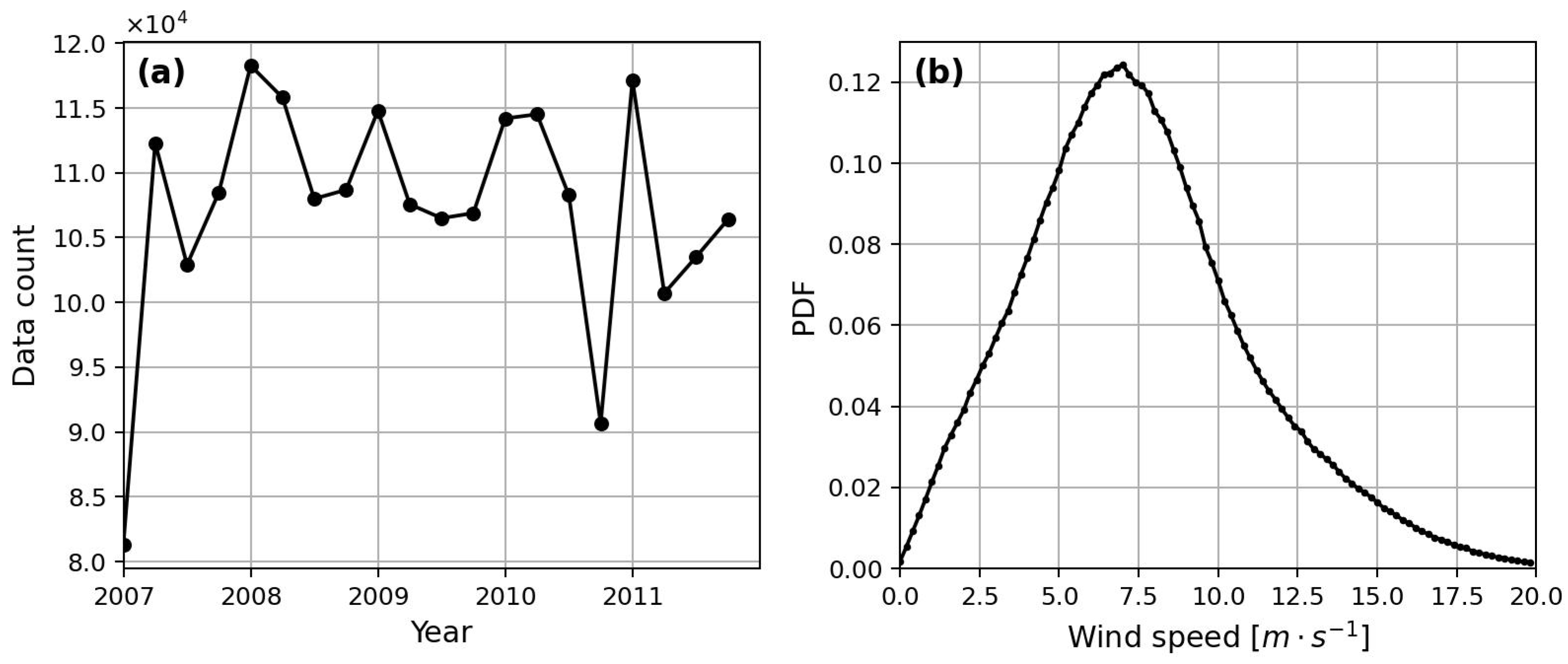
2.1. Envisat/ASAR Wave Mode

Envisat/ASAR, a radar system developed by European Space Agency (Paris, France) operating at the C-band (radar frequency of 5.4 GHz), was in orbit over a period spanning from November 2002 to April 2012. During its operational phase, it functioned across various modes to capture SAR images. Among these modes, the wave mode is designed specifically to collect observations of global ocean waves [25]. This mode acquires vignettes at a interval of 100 km along the satellite orbit, each with a footprint of 10 km × 7 km and spatial spacing of 9 m × 6 m. For our purposes, the wave mode imagettes obtained at 23° incidence and VV polarization are included here.
To conduct our analysis, SAR image cross-spectra annotated in the Level-1B products were employed. These products have been systematically processed from single look complex (SLC) SAR vignettes. Each image spectrum is constructed with 24 discrete wavenumbers, ranging from 0.008 rad·m 1 to 0.2 rad·m 1 , and 36 directions [26]. The ASAR wave mode data captured between January 2007 and December 2011 were spatially and temporally aligned with the European Centre for Medium-Range Weather Forecasts (ECMWF) reanalysis winds. This product is distributed at a longitude/latitude spacing of 0.5° with a temporal resolution of 6 h and served as a crucial reference. For each SAR image, the wind vector at the nearest distance and the time of SAR passage were taken for the collocated wind field. This comprehensive integration of ASAR wave mode data and ECMWF reanalysis wind vectors enhanced the accuracy and reliability of our analysis.
The seasonal number of SAR images accumulated by the Envisat/ASAR wave mode is plotted in Figure 1a. Over the temporal period of interest, the seasonal data count exhibited a discernible pattern of fluctuation. In the initial two years, from 2007 to 2008, there was a steady increase in data, reflecting a growing trend in information collection. However, a notable shift occurred in 2009, as the data count experienced a modest decline. This deviation may be attributed to various factors, such as changes in data collection strategies or shifts in priorities. The collocated wind speed probability density function (PDF) is depicted in Figure 1b with the speed bin set as 0.2 m · s 1 . A notable feature is the discernible nonuniformity in the distribution of the data points. The overall distribution roughly follows a Weibull curve, as with most of the wind speed distribution [27]. The peak is observed around 7 m · s 1 and there are far fewer data points beyond a wind speed of 15 m · s 1 . It is worth pointing out that the collocated wind speed comes from the reanalysis wind product, and the wind speed distribution is relatively smoother compared to satellite observations [28,29].

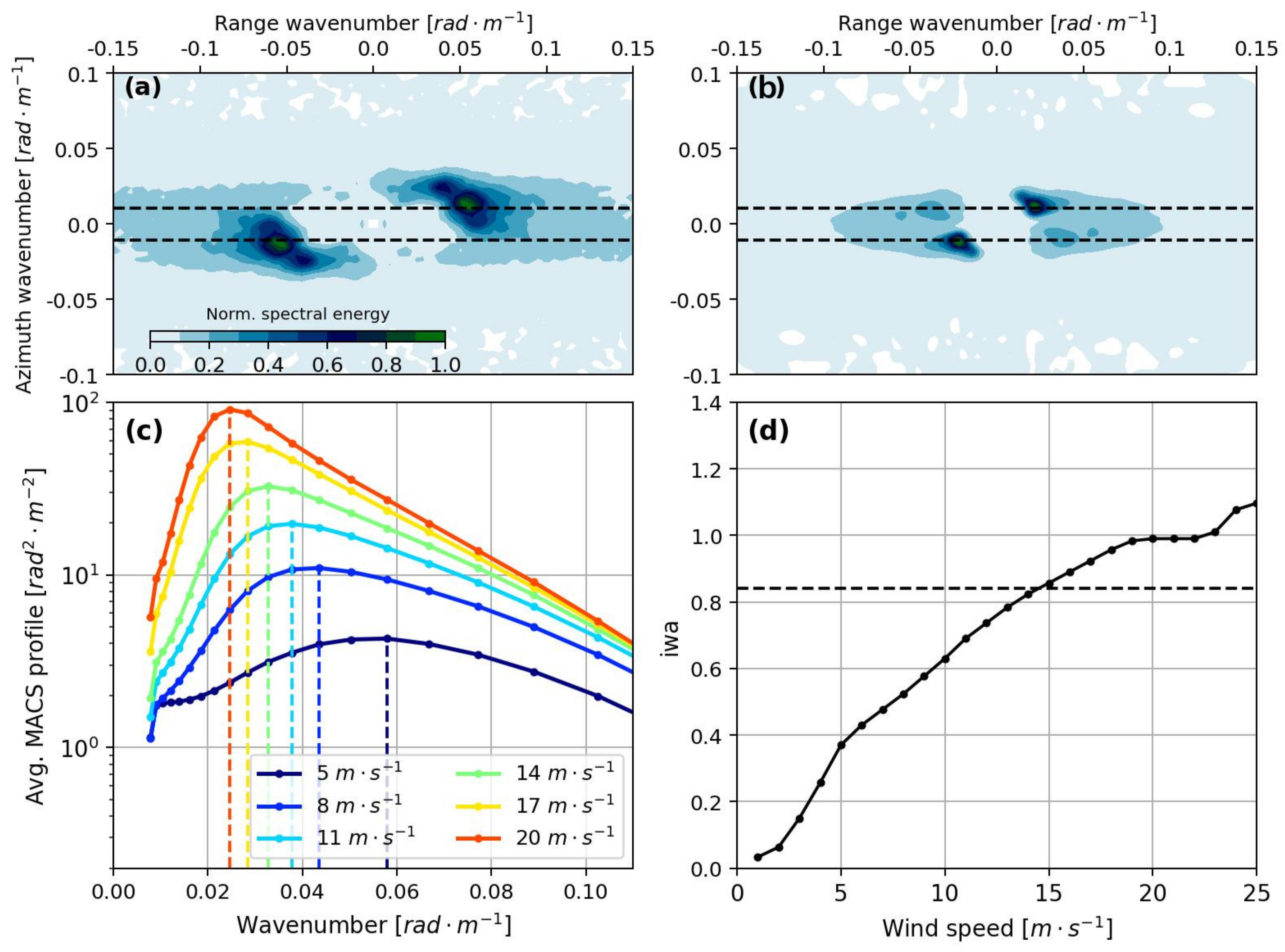
2.2. MACS Profile and Range Peak Wavenumber

As the SAR imaging principle of the ocean waves is strongly nonlinear, it introduces challenges in retrieving information for waves propagating in the flight direction, resulting in a loss of valuable data [30,31]. Existing efforts to estimate the significant wave height from SAR images are considered as a means to address this complexity [32,33]. However, wave spectra retrieval remains constrained by the inherent complexity of the process. Besides these challenges, the inclusion of external wind fields also introduces biases into the derived ocean wave spectra [30]. To circumvent the complexities of the inversion algorithms associated with nonlinear SAR imaging, we take a novel approach by extending the mean cross-spectrum (MACS) along the radar line-of-sight direction, as introduced in [23]. Two case examples are selected: one is acquired at relatively low wind speed of 5.2 m · s 1 , as plotted in Figure 2a, and the other at a wind speed of 11.1 m · s 1 , as in Figure 2b. The SAR image cross-spectrum example is presented at Cartesian coordinates with the abscissa being the range wavenumber and the ordinate being the azimuth wavenumber. The peak wavenumber in Figure 2a is identified around 0.06 rad · m 1 and this value reads 0.02 rad · m 1 in Figure 2b, associated with the different wind speeds. The nonlinear mapping is evident as the image spectrum is suppressed within a certain azimuth wavenumber, quantified as the azimuth cutoff. The definition area of MACS is presented in Figure 2a,b. The MACS profile is taken as the averaged cross-spectrum over the azimuth wavenumber from 2 π / 600 rad · m 1 to 2 π / 600 rad · m 1 as bounded by the two dashed horizontal lines at discrete range wavenumbers. Compared to the initial definition in [23], at a fixed range wavenumber, the extension encompasses a broad spectrum of ocean waves from wind seas to long ocean swells. The objective is to derive a range profile of SAR image cross-spectra, hereafter referred to as the MACS profile. By extending the MACS analysis across various wavenumbers, this approach aims to provide a comprehensive understanding of the ocean wave characteristics, capturing the nuances from wind-generated waves to the more persistent ocean swells. This strategy not only mitigates the nonlinear challenges inherent in SAR mapping but also attempts to minimize the biases introduced by external factors such as the input wind parameters.
Figure 2c gives the average MACS profiles at various wind speeds. For a given wind speed, the MACS profile roughly follows a bell shape that is left-skewed, resembling the one-dimensional wave spectrum [34]. The MACS rises gradually from either side of the peak and reaches its maximum at the peak wavenumber. The MACS magnitude at a fixed high wavenumber (vertical representation) first increases with the wind speed and then remains unchanged despite the increasing wind speed. This is associated with the development of local waves influenced by local winds, growing with the wind duration until the equilibrium state. This observation is particularly evident for shorter waves, as the MACS profiles cluster together at larger wavenumbers; see in Figure 2c. The wavenumber with the maximum energy along the MACS profile is identified as the range peak wavenumber, as illustrated in [24]. As the wind speed increases, the detected range peak wavenumber shifts toward smaller values, corresponding to longer ocean waves. This is consistent with the wave development theory, positing that the local wind–wave coupling is characterized by the inverse wave age (iwa) parameter. This parameter is expressed as the ratio of the wind speed to the phase speed of peak waves c p = g / k , with g being the gravitational acceleration and k the wavenumber. It has been broadly used to represent the degree of wave development with local wind forcing [10,35]. The threshold of 0.84 is typically employed to characterize the equilibrium sea state, with lower iwa values for ocean swell and larger values for wind seas. Despite the common practice of considering the wind fetch and duration in addressing the wind–wave coupling [36,37], it should be pointed out that these two factors are difficult and impractical to obtain from satellite observations. As a demonstration, only the wind speed is taken into account to estimate the iwa parameter. Figure 2d presents the variation in the iwa relative to the wind speed obtained from the averaged MACS profile in Figure 2c. As shown, the iwa gradually increases with the wind speed, indicating a shift from swell dominance at low winds to wind sea dominance at higher winds. This pattern is in qualitative agreement with the results based on reanalysis models [10], which makes the SAR range MACS profile a valuable additional means of examining the local wind–wave coupling.
To better demonstrate the detection of the range peak wavenumber based on the MACS profile, four cases are selected from the database, as shown in Figure 3a. All cases are chosen with similar wind speeds and various iwa values to demonstrate the variation in range peak wavenumbers. The index of each case is arranged in terms of decreasing iwa from case 1 to case 4. Neglecting the wind speed deviation, the range peak wavenumber increases with the iwa. This is consistent with the understanding that a smaller iwa corresponds to older and longer waves, while a higher iwa corresponds to younger and shorter waves. To facilitate an understanding from a theoretical point of view, we take advantage of the Elfouhaily spectrum proposed in [34] to examine the relationship between the iwa and the peak wavenumber, as a fully developed sea state is uncommon in reality. The varying iwa produces differences in the dominance of swell and wind waves, leading to various peak wavenumbers, as shown in Figure 3b. For example, at the wind speed of 10 m · s 1 , the peak wavenumber increases from 0.016 rad · m 1 to 0.141 rad · m 1 as the iwa increases from 0.4 to 0.8, which corresponds to the wavelength shortening from 387 m to 44 m. As such, each individual MACS profile will deviate from the average case in terms of the development degree of the local sea state as characterized by the iwa parameter.

3. Results and Discussion

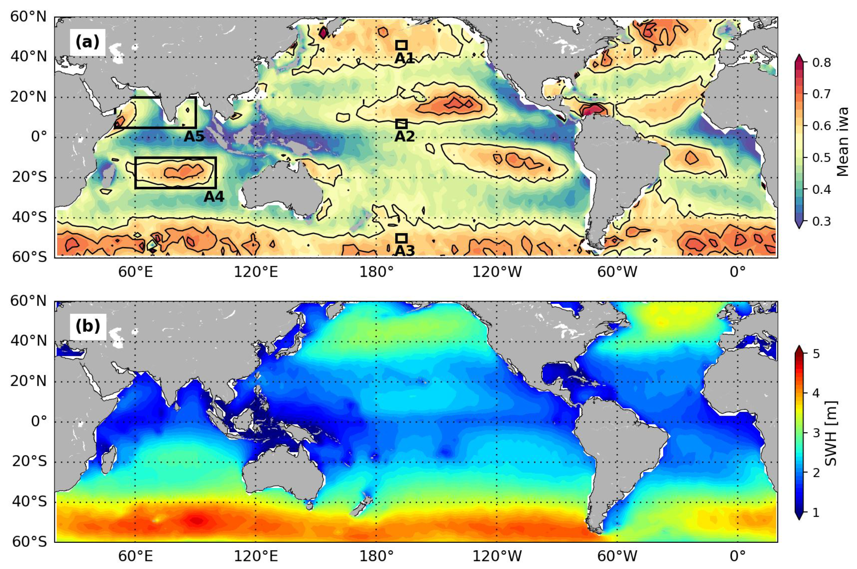
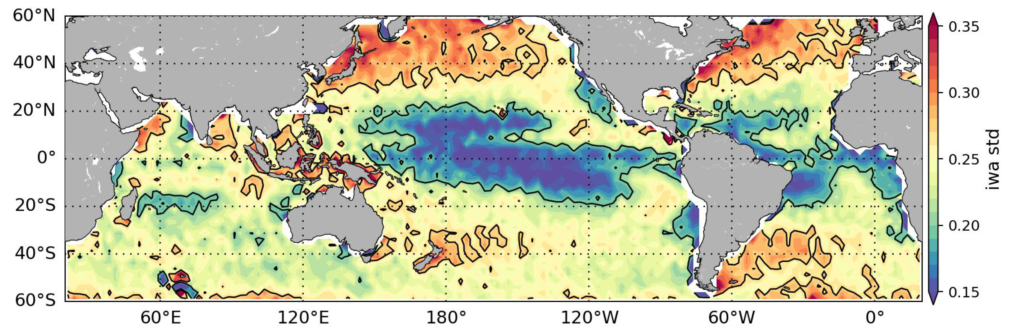
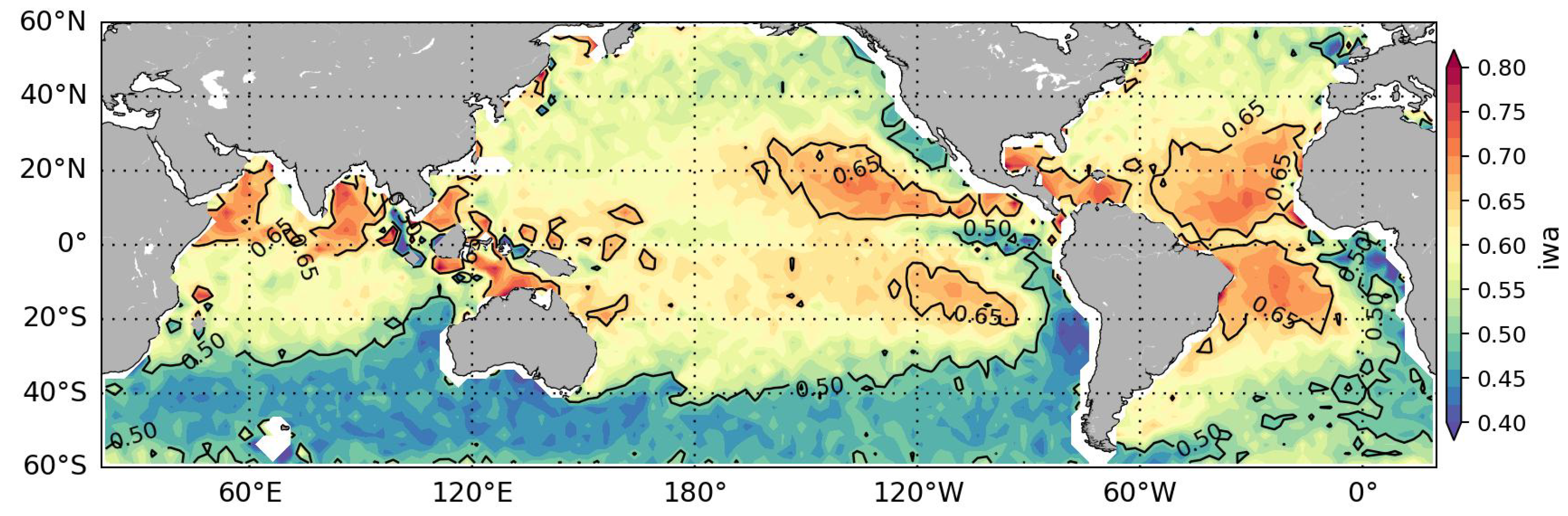
3.1. Global Characteristics of SAR-Derived iwa

Extensive research has consistently highlighted the prevalence of underdeveloped to developed sea states, particularly in the presence of high wind conditions [10,12], as depicted in Figure 4a. The mean pattern indicates that most of the ocean basin has an iwa value no larger than 0.8, consistent with the results obtained based on the long-term reanalysis data [10]. As shown, storm tracks are the areas with the largest iwa values. Given that fact that higher iwa values indicate stronger coupling, waves in the storm tracks extract greater momentum from the wind to grow. As the waves generated by storms propagate away from their origin, they transform into swells with limited coupling to local winds, a phenomenon that is well documented in the literature [18,38,39]. This scenario is notably prevalent in trade wind regions, characterized by lower iwa values approximately around 0.5 (depicted by the light yellow color in Figure 4a). While such trends generally hold, exceptions exist. For instance, the Gulf of Mexico stands out, with a relatively high iwa of 0.75, attributed to its semi-enclosed nature and the consequently shorter wind fetch. For comparison, the mean significant wave height (SWH) averaged over the same temporal duration as the Envisat/ASAR acquisitions is plotted in Figure 4b. Note that the significant wave height product is obtained from the Copernicus Marine Environment Monitoring Service (CMEMS). The Level 4 reprocessed SWH is available on a daily basis with a spatial bin of 2° along both the latitude and longitude. Overall, the global pattern observed in the SWH distribution is in good agreement with that of the iwa. For instance, high values are found in the extratropics in both hemispheres, as well as in the trade winds. The dissimilarities primarily occur in semi-closed seas with low SWH values but a high iwa. This is anticipated because the waves over these regions are mostly derived from young seas generated by limited wind fetch and durations. Their difference is a significant indicator to consider the iwa in describing the local sea state, in addition to the commonly used wind speed and wave height.
The global distribution of the standard deviation of the iwa over a grid of 2.5° along both the longitude and latitude is presented in Figure 5. In general, the spatial pattern of the standard deviation is quite different from that of the mean iwa, as shown in Figure 4. In particular, the southern ocean emerges as a region with year-round consistency in the iwa, characterized by relatively small variability. The lowest standard deviation is observed in the trade winds, indicating the steady iwa over this region. This is expected given the consistent dominance of ocean swell in this area [12]. The northern extratropics show relatively high variability in both the Pacific Ocean and the Atlantic Ocean. This is associated with the strong seasonal variation in winds, as high winds occur in winter and low winds in summer. In addition, a strong standard deviation is also observed in the Arabian Sea and the Bay of Bengal, due to the wind reversal in the monsoon season.

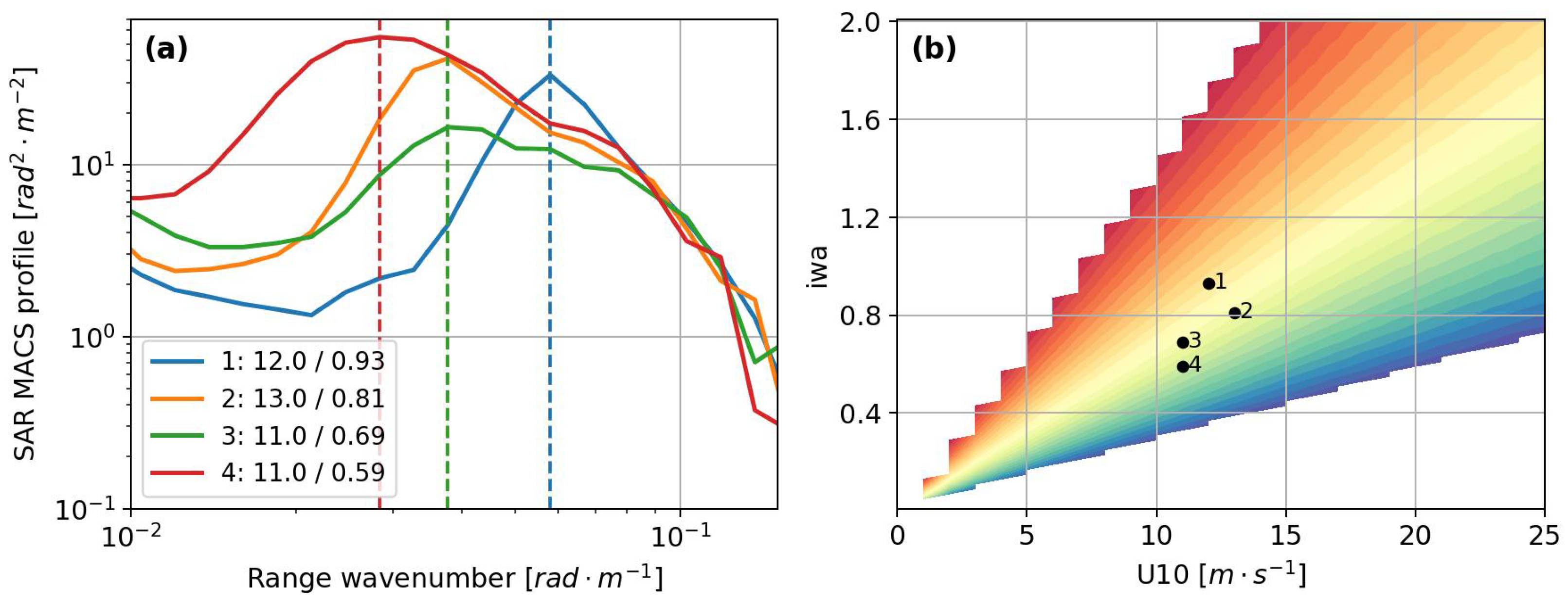
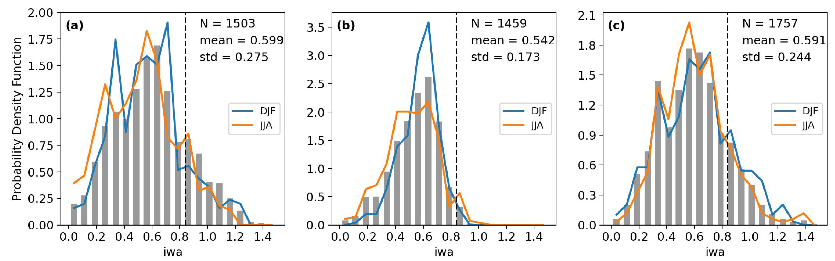
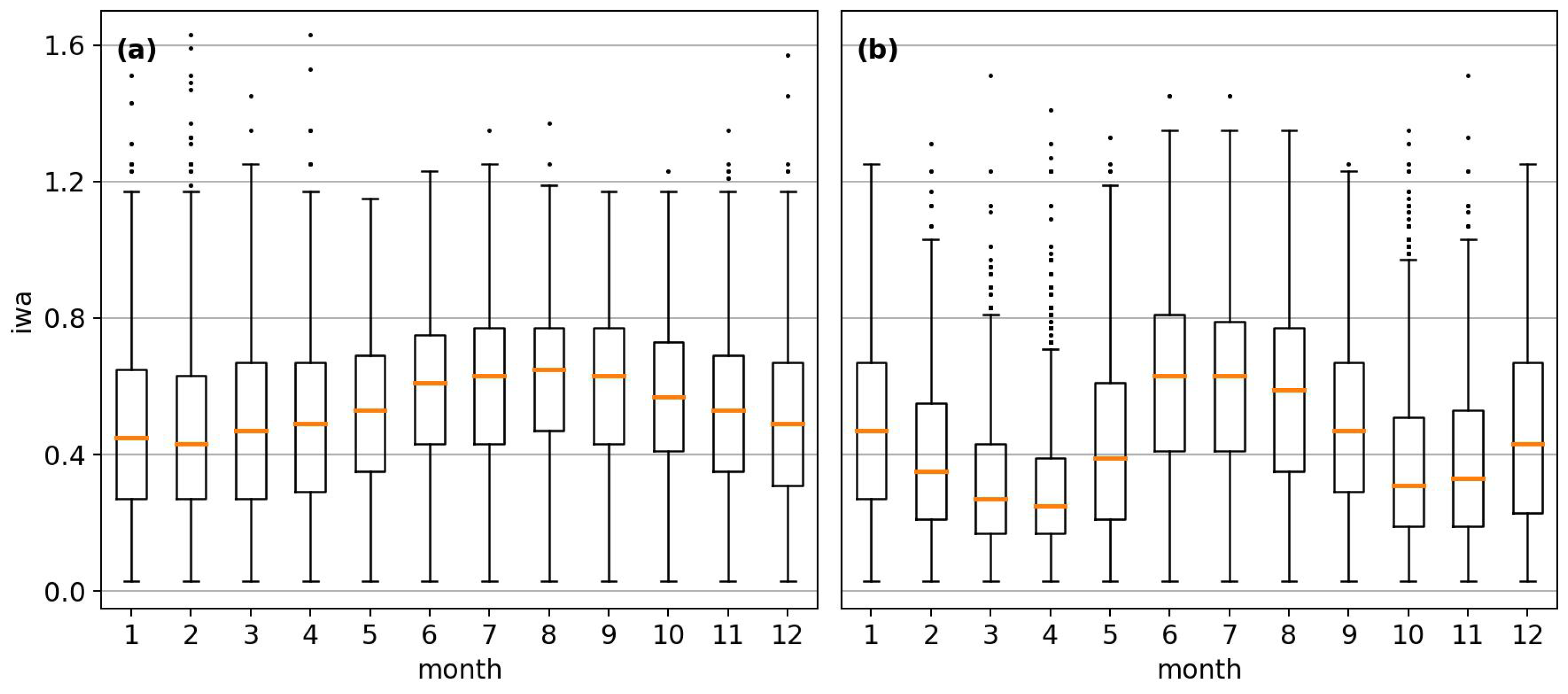
3.2. Local Variation in iwa

To look into the local characteristics of the iwa, we have identified five chosen regions of interest (ROIs), as illustrated in Figure 4. Notably, three of these ROIs are positioned along the 180° longitude line, encompassing latitudes of 46° N, 7° N, and 50° S. Each of these ROIs spans a latitude and longitude bin of 4°. This selection is made to capture and illustrate the mean and variability within the extratropical and trade wind regions. By focusing on these specific latitudinal points, we aim to provide a comprehensive portrayal of the local characteristics of the iwa in these distinct climatic zones. Complementing this extratropical emphasis, the remaining two ROIs have been placed in the Indian Ocean, strategically chosen to highlight the temporal variability of the iwa induced by the summer monsoon in this specific geographical area. This region holds significance due to the pronounced influence of the seasonal monsoonal patterns on oceanic conditions.
Figure 6 gives the probability density function (PDF) of the iwa over ROI A1. The bar denotes the overall PDF and the colored curves are the seasonal PDFs in winter (blue) and in summer (orange), respectively. A1 has a mean iwa of 0.584 with a standard deviation of 0.296. This is representative of the high wind conditions in the northern extratropics and relatively stronger seasonality. In winter, the northern extratropics see the frequent occurrence of storms, bringing consistently high winds and less developed sea states. By contrast, during JJA, this region is characterized by low winds and long ocean swells, propagated from the far southern ocean, leading to a relatively low iwa. Such seasonal variation is well captured by the blue and the orange curves. In comparison, the other two ROIs, A2 and A3, as shown in Figure 6b,c, show a weaker standard deviation associated with the consistently low winds in A2 and high winds in A3, respectively. The iwa PDF is almost overlapped between the summer and the winter. In other words, the iwa, as an indicator of the degree of wave development, is worth investigation not only from the perspective of its mean state but also its variability at a given geographical location.
The box plots depicting the monthly variations in the iwa over the two distinct ROIs of A4 and A5 are presented in Figure 7. Remarkably, both ROIs exhibit discernible seasonality with distinctive patterns. In the case of A4, an observable trend shows increasing iwa values from January, peaking in August and subsequently dropping until December. It is noteworthy that the monthly mean iwa values consistently fall within the range of [0.4, 0.7], evidencing the robustness of this seasonally driven pattern. The spread of the iwa values, characterized by the upper (75th) and lower (25th) quantiles, remains relatively stable throughout the year, contributing to the coherence of the observed seasonality. In contrast, the monthly iwa variation over A5 depicts a distinct temporal trend when compared to A4. Here, the mean iwa follows a roughly cosine shape, reaching its peak in January and July, while reaching its trough in March and October. This unique pattern is likely attributed to the seasonal reversal of the winds, transitioning from winter to the summer monsoon. The distinct pattern of the iwa in A5 evidences the significant influence of seasonal wind patterns on the local characteristics of ocean waves.

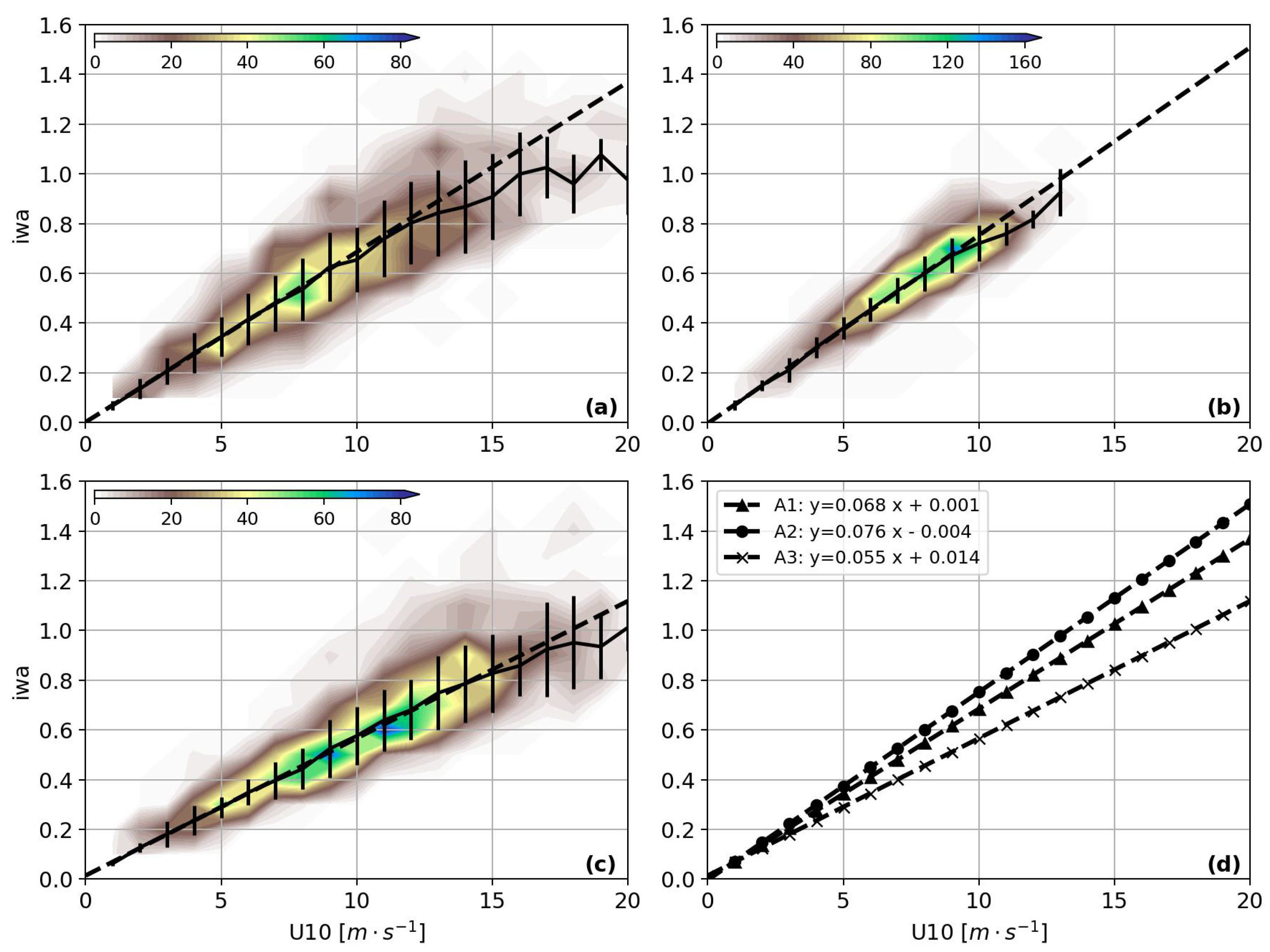
3.3. Analysis of Wind–Wave Interaction

In the exploration of wind–wave interactions, the relationship between the iwa and the wind speed serves as a crucial parameter. Three distinct plots, each representing a unique geographical location as annotated in Figure 4, are given in Figure 8 to show their detailed relationships. While all three plots reveal a linear trend, the subtle differences in slope across these locations offer valuable insights into the varying degrees of coupling between wind and waves. Figure 8a denotes the relationship over the ROI A1, situated in the northern storm track, showing a linear relationship between the iwa and U10. This region is characterized by high wind speeds brought by winter storms, implying robust coupling between the wind and waves. In Figure 8b, representative of a trade wind region, the linear trend between the iwa and U10 takes on a slightly steeper slope. Trade wind regions are known for their more stable and consistent winds, resulting in waves with less dependence on the wind momentum. The steeper slope in this plot indicates that the waves in trade wind regions extract comparatively more energy from the wind. Figure 8c presents the relationship over ROI A3 in the southern storm tracks. The plot reveals the lowest slope, indicative of the consistent presence of ocean swell in this region due to the high winds throughout the year. This plot highlights the distinct nature of the wind–wave interaction in high seas, where geographical constraints play a significant role in shaping the coupling dynamics between the wind and waves. Examining these three plots collectively underscores the diversity of wind–wave interactions across different geographical contexts, as in Figure 8d. The variations in slope reveal the sensitivity of the iwa–U10 relationship to the local environmental conditions. At a specific wind speed, region A2, influenced by trade winds, exhibits a higher iwa, indicative of younger seas generated by local wind activity. This occurrence may be ascribed to waves spreading along their path of propagation, causing shorter wind-driven waves to become the spectral peak, consequently resulting in higher iwa values. In contrast, regions A1 and A3, situated over the extratropics, are characterized by longer peak wavelengths and lower iwa values. This distinction highlights the variability in sea states among different regions at a given wind speed.
The global map of the iwa at a consistent wind speed of 8 m · s 1 is shown in Figure 9, providing a comprehensive snapshot of the dynamic interaction between the wind and waves across the ocean basins. At this specific wind speed, the map reveals distinct spatial patterns in the iwa, serving as a visual representation of the strength of the coupling between the wind and waves on a global scale. Regions with higher iwa values signify a more robust interaction, indicating that the waves in these areas require increased momentum from the wind to reach significant heights. Higher values are typically observed in the trade winds, where the winds are moderate throughout the year, as bounded by the iwa contour of 0.65 as shown. Conversely, lower iwa values suggest weaker coupling, signifying waves that are less dependent on wind energy for their development. Lower values are found in the southern ocean, typically bounded by the iwa contour of 0.5. This map offers insights into the variability of the wind–wave dynamics across different oceanic regions, contributing to a deeper understanding of the complex interaction between the atmospheric and oceanic processes.

4. Conclusions

An enhanced understanding of ocean wave characteristics is important given that the exchange of momentum in the air–sea interaction is transferred via the sea surface waves. The parameterization of flux transfer to achieve better global numerical atmosphere–ocean coupled models should account for the sea state impact, as pointed out in [40]. This advancement is expected to be realized with the extended exploitation of existing data for wave climate studies, as emphasized in [41]. Spaceborne satellite observations have emerged as valuable tools in exploring the global wave climate [12,42]. Notably, the great potential of high-resolution SAR measurements capable of capturing ocean wave spectral signatures may have been previously underestimated. A decade of data acquisition by the Envisat/ASAR wave mode enables the examination of global ocean wave characteristics. Our approach, in contrast to utilizing integrated wave variables, illustrates promising results by specifically focusing on the range-traveling ocean waves.
Ocean waves primarily interact with local winds, and the MACS profile demonstrates a higher degree of coupling between the ocean swell and increased wind speeds. The extent of this coupling, crucial in understanding wave development, is notably characterized by the iwa parameter. Despite its qualitative nature, the degree of wind–wave coupling derived from MACS holds significance. Utilizing precise wind data independently obtained from an SAR image enables a comprehensive exploration of wind–wave coupling at the global scale. Specifically, the investigation of the wind–wave interaction during tropical cyclones stands out as an area worthy of dedicated efforts.
In this study, we investigated the spatial and temporal variability of the SAR-derived iwa. These results not only offer a comprehensive view of the present state of the sea surface but also enable the tracking of temporal variations, facilitating the study of seasonal and long-term trends. The insights gained from the SAR-derived iwa have implications for various fields, including climate research, oceanography, and maritime applications. As SAR technology continues to evolve, the potential for further advancements in understanding and predicting ocean wave dynamics is significant. Overall, the SAR-derived iwa contributes valuable information to our understanding of the complex interactions shaping the open oceans, paving the way for enhanced forecasting capabilities and the improved management of marine resources.

Author Contributions

Conceptualization, H.L.; methodology, H.L.; formal analysis, H.L.; investigation, H.L. and Y.H.; writing—original draft preparation, H.L.; writing—review and editing, H.L. and Y.H.; supervision, Y.H. All authors have read and agreed to the published version of the manuscript.

Funding

This research was funded by the National Natural Science Foundation of China under grants 42006163 and 42027805.

Institutional Review Board Statement

Not applicable.

Informed Consent Statement

Not applicable.

Data Availability Statement

The Envisat ASAR product is publicly available at https://earth.esa.int/ (accessed on 1 December 2023) upon request. The significant wave height product is publicly available at https://data.marine.copernicus.eu/ (accessed on 1 December 2023).

Acknowledgments

We would like to acknowledge the European Space Agency for making the Envisat/ASAR products available and the Copernicus Marine Service for providing the merged significant wave height product.

Conflicts of Interest

The authors declare no conflicts of interest.

References

  1. Toba, Y. Local balance in the air-sea boundary processes. J. Oceanogr. 1972, 28, 109–120. [Google Scholar] [CrossRef]
  2. Phillips, O.M. The Dynamics of the Upper Ocean, 2nd ed.; Cambridge University Press: Cambridge/London, UK; New York, NY, USA; Melbourne, Australia, 1977. [Google Scholar]
  3. Hasselmann, K.; Barnett, T.; Bouws, E.; Carlson, H.; Cartwright, D.; Enke, K.; Ewing, J.; Gienapp, H.; Hasselmann, D.; Kruseman, P.; et al. Measurements of wind-wave growth and swell decay during the Joint North Sea Wave Project (JONSWAP). In Part of Collection: Hydraulic Engineering Reports A(8), 12; Deutches Hydrographisches Institut: Hamburg, Germany, 1973. [Google Scholar]
  4. Sterl, A.; Komen, G.J.; Cotton, P.D. Fifteen years of global wave hindcasts using winds from the European Centre for Medium-Range Weather Forecasts reanalysis: Validating the reanalyzed winds and assessing the wave climate. J. Geophys. Res. Ocean. 1998, 103, 5477–5492. [Google Scholar] [CrossRef]
  5. Young, I. Seasonal variability of the global ocean wind and wave climate. Int. J. Climatol. 1999, 19, 931–950. [Google Scholar] [CrossRef]
  6. Wang, X.L.; Zwiers, F.W.; Swail, V.R. North Atlantic Ocean Wave Climate Change Scenarios for the Twenty-First Century. J. Clim. 2004, 17, 2368–2383. [Google Scholar] [CrossRef]
  7. Li, X.; Lehner, S.; Bruns, T. Ocean Wave Integral Parameter Measurements Using Envisat ASAR Wave Mode Data. IEEE Trans. Geosci. Remote Sens. 2011, 49, 155–174. [Google Scholar] [CrossRef]
  8. Young, I.R.; Zieger, S.; Babanin, A.V. Global Trends in Wind Speed and Wave Height. Science 2011, 332, 451–455. [Google Scholar] [CrossRef] [PubMed]
  9. Young, I.R.; Ribal, A. Multiplatform evaluation of global trends in wind speed and wave height. Science 2019, 364, 548–552. [Google Scholar] [CrossRef] [PubMed]
  10. Hanley, K.E.; Belcher, S.E.; Sullivan, P.P. A Global Climatology of Wind–Wave Interaction. J. Phys. Oceanogr. 2010, 40, 1263–1282. [Google Scholar] [CrossRef]
  11. Stopa, J.E.; Cheung, K.F.; Tolman, H.L.; Chawla, A. Patterns and cycles in the Climate Forecast System Reanalysis wind and wave data. Ocean Model. 2013, 70, 207–220. [Google Scholar] [CrossRef]
  12. Chen, G.; Chapron, B.; Ezraty, R.; Vandemark, D. A Global View of Swell and Wind Sea Climate in the Ocean by Satellite Altimeter and Scatterometer. J. Atmos. Ocean. Technol. 2002, 19, 1849–1859. [Google Scholar] [CrossRef]
  13. Jiang, H.; Chen, G. A Global View on the Swell and Wind Sea Climate by the Jason-1 Mission: A Revisit. J. Atmos. Ocean. Technol. 2013, 30, 1833–1841. [Google Scholar] [CrossRef]
  14. Shimura, T.; Mori, N.; Mase, H. Future Projections of Extreme Ocean Wave Climates and the Relation to Tropical Cyclones: Ensemble Experiments of MRI-AGCM3.2H. J. Clim. 2015, 28, 9838–9856. [Google Scholar] [CrossRef]
  15. Reguero, B.G.; Losada, I.J.; Méndez, F.J. A recent increase in global wave power as a consequence of oceanic warming. Nat. Commun. 2019, 10, 205. [Google Scholar] [CrossRef]
  16. Portilla-Yandún, J. The Global Signature of Ocean Wave Spectra. Geophys. Res. Lett. 2018, 45, 267–276. [Google Scholar] [CrossRef]
  17. Portilla-Yandún, J.; Salazar, A.; Cavaleri, L. Climate patterns derived from ocean wave spectra. Geophys. Res. Lett. 2016, 43, 11736–11743. [Google Scholar] [CrossRef]
  18. Collard, F.; Ardhuin, F.; Chapron, B. Monitoring and analysis of ocean swell fields from space: New methods for routine observations. J. Geophys. Res. Ocean. 2009, 114, 1–15. [Google Scholar] [CrossRef]
  19. Stopa, J.E.; Ardhuin, F.; Husson, R.; Jiang, H.; Chapron, B.; Collard, F. Swell dissipation from 10 years of Envisat advanced synthetic aperture radar in wave mode. Geophys. Res. Lett. 2016, 43, 3423–3430. [Google Scholar] [CrossRef]
  20. Ardhuin, F.; Collard, F.; Chapron, B.; Girard-Ardhuin, F.; Guitton, G.; Mouche, A.; Stopa, J.E. Estimates of ocean wave heights and attenuation in sea ice using the SAR wave mode on Sentinel-1A. Geophys. Res. Lett. 2015, 42, 2317–2325. [Google Scholar] [CrossRef]
  21. Stopa, J.E.; Sutherland, P.; Ardhuin, F. Strong and highly variable push of ocean waves on Southern Ocean sea ice. Proc. Natl. Acad. Sci. USA 2018, 115, 5861–5865. [Google Scholar] [CrossRef]
  22. Li, X.M. A new insight from space into swell propagation and crossing in the global oceans. Geophys. Res. Lett. 2016, 43, 5202–5209. [Google Scholar] [CrossRef]
  23. Li, H.; Chapron, B.; Mouche, A.; Stopa, J.E. A New Ocean SAR Cross-Spectral Parameter: Definition and Directional Property Using the Global Sentinel-1 Measurements. J. Geophys. Res. Ocean. 2019, 124, 1566–1577. [Google Scholar] [CrossRef]
  24. Li, H.; He, Y.; Wang, C.; Lin, W.; Yang, J. Study of global ocean waves based on SAR image cross-spectrum. Haiyang Xuebao 2023, 46, 1–7. (In Chinese) [Google Scholar]
  25. Hasselmann, K.; Chapron, B.; Aouf, L.; Ardhuin, F.; Collard, F.; Engen, G.; Hasselmann, S.; Heimbach, P.; Janssen, P.; Johnsen, H.; et al. The ERS SAR Wave Mode—A Breakthrough in global ocean wave observations. In ERS Missions—20 Years of Observing Earth; European Space Agency: Paris, France, 2012. [Google Scholar]
  26. Johnsen, H. ENVISAT ASAR Wave Mode Product Description and Reconstruction Procedure. In Technical Report 1/2005; Norut: Tromso, Norway, 2005. [Google Scholar]
  27. Escobar, C.A.; Restrepo Alvarez, D. Estimation of global ocean surface winds blending reanalysis, satellite and buoy datasets. Remote Sens. Appl. Soc. Environ. 2023, 32, 101012. [Google Scholar] [CrossRef]
  28. Zhao, K.; Zhao, C. Evaluation of HY-2A Scatterometer Ocean Surface Wind Data during 2012–2018. Remote Sens. 2019, 11, 2968. [Google Scholar] [CrossRef]
  29. Ribal, A.; Young, I.R. Global Calibration and Error Estimation of Altimeter, Scatterometer, and Radiometer Wind Speed Using Triple Collocation. Remote Sens. 2020, 12, 1997. [Google Scholar] [CrossRef]
  30. Engen, G.; Johnsen, H. SAR-ocean wave inversion using image cross spectra. IEEE Trans. Geosci. Remote Sens. 1995, 33, 1047–1056. [Google Scholar] [CrossRef]
  31. Chapron, B.; Johnsen, H.; Garello, R. Wave and wind retrieval from sar images of the ocean. Ann. Télécommun. 2001, 56, 682–699. [Google Scholar] [CrossRef]
  32. Schulz-Stellenfleth, J.; König, T.; Lehner, S. An empirical approach for the retrieval of integral ocean wave parameters from synthetic aperture radar data. J. Geophys. Res. Ocean. 2007, 112, 1–14. [Google Scholar] [CrossRef]
  33. Stopa, J.E.; Mouche, A. Significant wave heights from Sentinel-1 SAR: Validation and applications. J. Geophys. Res. Ocean. 2017, 122, 1827–1848. [Google Scholar] [CrossRef]
  34. Elfouhaily, T.; Chapron, B.; Katsaros, K.; Vandemark, D. A unified directional spectrum for long and short wind-driven waves. J. Geophys. Res. Ocean. 1997, 102, 15781–15796. [Google Scholar] [CrossRef]
  35. Jiang, H.; Chen, G.; Yu, F. An index of wind–wave coupling and its global climatology. Int. J. Climatol. 2016, 36, 3139–3147. [Google Scholar] [CrossRef]
  36. Hwang, P.A. Duration- and fetch-limited growth functions of wind-generated waves parameterized with three different scaling wind velocities. J. Geophys. Res. Ocean. 2006, 111, 1–10. [Google Scholar] [CrossRef]
  37. Young, I.; Vinoth, J. An “extended fetch” model for the spatial distribution of tropical cyclone wind–waves as observed by altimeter. Ocean Eng. 2013, 70, 14–24. [Google Scholar] [CrossRef]
  38. Kudryavtsev, V.; Yurovskaya, M.; Chapron, B. Self-Similarity of Surface Wave Developments Under Tropical Cyclones. J. Geophys. Res. Ocean. 2021, 126, e2020JC016916. [Google Scholar] [CrossRef]
  39. Hell, M.C.; Ayet, A.; Chapron, B. Swell Generation Under Extra-Tropical Storms. J. Geophys. Res. Ocean. 2021, 126, e2021JC017637. [Google Scholar] [CrossRef]
  40. Janssen, P.A.E.M.; Viterbo, P. Ocean Waves and the Atmospheric Climate. J. Clim. 1996, 9, 1269–1287. [Google Scholar] [CrossRef]
  41. Hemer, M.A.; Wang, X.L.; Weisse, R.; Swail, V.R. Advancing Wind-Waves Climate Science. Bull. Am. Meteorol. Soc. 2012, 93, 791–796. [Google Scholar] [CrossRef]
  42. Stopa, J.E.; Ardhuin, F.; Chapron, B.; Collard, F. Estimating wave orbital velocity through the azimuth cutoff from space-borne satellites. J. Geophys. Res. Ocean. 2015, 120, 7616–7634. [Google Scholar] [CrossRef]
Figure 1. (a) Seasonal data count of the Envisat/ASAR wave mode images included in this study; (b) the wind speed probability density function (PDF) at a speed bin of 0.2 m · s 1 .
Jmse 12 00433 g001
Figure 2. Two examples of SAR image cross-spectra with color representing the normalized spectral energy relative to the maximum value in (a,b). The dashed horizontal lines mark the boundary over which the azimuth wavenumber is averaged to obtain the range MACS profile. (c) Mean MACS profile at different wind speeds. The vertical curve is the detected range peak wavenumber from the corresponding MACS profile. (d) Variation in iwa relative to the wind speed obtained from the average MACS profile.
Jmse 12 00433 g002
Figure 3. (a) Four MACS profiles selected with different combinations of wind speed and iwa, with the values annotated in the legend. The vertical dashed lines are the detected range peak wavenumbers with the two cases of 2 and 3 overlapped. (b) Variation in peak wavenumber with both wind speed and iwa derived from the Elfouhaily wave spectrum [34]. The color gives the estimated peak wavenumber with the four selected cases annotated in the plot. Locations of the four example cased in (a) are also labeled in this plot.
Jmse 12 00433 g003
Figure 4. (a) Global average of SAR-derived iwa at a bin of 2.5° by 2.5° along the latitude and longitude axis. Five regions of interest are marked in the plot for subsequent analysis. (b) Global mean significant wave height derived from multiple altimeters over the same period of SAR acquisition at a spatial bin of 2°. Five region of interests indexed by A1–A5 are plotted in the figure for subsequent analysis.
Jmse 12 00433 g004
Figure 5. Same as in Figure 4 but for standard deviation of the iwa.
Jmse 12 00433 g005
Figure 6. Probability density function (PDF) of iwa over the ROIs of (a) A1, (b) A2, and (c) A3 annotated in Figure 3. The vertical bar denotes the overall PDF of iwa and the solid curves are the seasonal PDFs in December–January–February (DJF) and in June–July–August (JJA), respectively. The vertical dashed line represents the iwa of 0.84 corresponding to the fully developed sea.
Jmse 12 00433 g006
Figure 7. Monthly box plot of iwa over ROIs (a) A4 and (b) A5 as annotated in Figure 3. The upper and lower boundaries of the box represent the first and the third quartile, respectively. The horizontal line in orange is the mean value in each month.
Jmse 12 00433 g007
Figure 8. The relationship of iwa versus the wind speed U10 at the three ROIs of (a) A1, (b) A2, (c) A3. The color gives the data count with a bin of 1 m · s 1 for a wind speed and iwa bin of 0.1, respectively. The solid curve in each plot is the linear fit and the error bar is the standard deviation at each wind speed. (d) presents the three linear fits with the regression slope annotated in the upper-left corner.
Jmse 12 00433 g008
Figure 9. The global map of iwa at wind speed of 8 m · s 1 ± 0.5 m · s 1 with bin of 2.5° along both the latitude and longitude axis, respectively.
Jmse 12 00433 g009
Disclaimer/Publisher’s Note: The statements, opinions and data contained in all publications are solely those of the individual author(s) and contributor(s) and not of MDPI and/or the editor(s). MDPI and/or the editor(s) disclaim responsibility for any injury to people or property resulting from any ideas, methods, instructions or products referred to in the content.

