Ship SINS/CNS Integrated Navigation Aided by LSTM Attitude Forecast

Abstract

Under the strong interference of sky background noise, the reliability of celestial navigation system (CNS) measurement will drop sharply, which leads to performance deterioration for ships’ strapdown inertial navigation system (SINS)/CNS integrated navigation. To solve this problem, a long short-term memory (LSTM) model is trained to forecast a ship’s attitude to detect the attitude provided by the CNS, and the LSTM forecasted attitude can also be used as a backup in case of CNS failure. First, the SINS/CNS integrated model is derived based on an attitude solution of the CNS, which provides more favorable feature data for LSTM learning. Then, the key techniques of LSTM modeling such as dataset construction, LSTM coding method, hyperparameter optimization and training strategy are described in detail. Finally, an experiment is conducted to evaluate the actual performance of the investigated methods. The results show that the LSTM model can accurately forecast a ship’s attitude: the horizon reference error is less than 0.5′ and the yaw error is less than 0.6′, which can provide reliable reference attitude for the SINS when the CNS is invalid.

1. Introduction

The SINS is an autonomous navigation system, with the advantages of strong anti-interference ability, good real-time performance and no geographical restrictions, which has become the main navigation system for all kinds of carriers [1,2]. However, due to the accumulation of position, speed and attitude errors over time, the SINS is difficult to use as an independent high-precision navigation system [3,4]. The CNS has the advantages of the non-accumulation of errors over time, strong autonomy, anti-interference ability and high reliability, but it is vulnerable to being affected by sky background noise and has disadvantages such as a low data rate and weak real-time performance and continuity [5,6,7]. Modern information-based navigation warfare has seriously threatened all kinds of radio navigation systems represented by satellite navigation systems [8]. The complex battlefield electromagnetic environment requires that navigation system must have strong autonomy and anti-interference ability. The SINS and CNS can not only meet the aforementioned requirements, but also have strong complementarities with each other [9,10]. Therefore, in recent years, SINS/CNS integrated navigation has been widely considered and rapidly developed. With great development potential and broad application prospects, the SINS/CNS has become an important direction of integrated navigation technology development [9].

A ship CNS works on the earth’s surface; due to harsh astronomical observation conditions, it will be interfered with by strong sky background noise. Even the high-resolution CNS with a small field of view has to face the problem of a sharp decline of observation accuracy and even observation interruption under the impact of atmospheric turbulence, clouds and other meteorological factors [11,12]. It is an urgent problem for SINS/CNS integrated navigation to keep the CNS in a stable working state and provide reliable navigation reference information for the SINS.

In recent years, recurrent neural networks (RNNs) have been widely used in dealing with time series problems, and they provide the inspiration for the investigation in this article. RNNs evolved from the Hopfield neural network proposed by Saratha Sathasivam in 1982, which embodies the idea that “human cognition is based on past experience and memory” [13,14]. The difference with ordinary Deep Neural Networks [15,16] and Convolutional Neural Networks [17,18] is that RNNs not only take into account the influence of the output of the previous moment on the current moment, but also have the memory of past content. Just like the human brain, they do not process and judge current information independently but make optimal choices based on previous knowledge and experience [19]. Therefore, RNNs have significant applicability in processing sequence data and solving serialization-related problems. At present, RNNs have been successfully applied in many artificial intelligence fields, such as Google voice search, Baidu deep speech recognition and Amazon-related products. However, as the length of the time series becomes longer, the memory ability of the RNN will rapidly deteriorate, resulting in “gradient vanishing” or “gradient explosion” [20,21]. As an evolutionary version of RNNs, long short-term memory (LSTM) adopts a gating mechanism and memory cells, which can flexibly control the retention degree of the historical information of time series and effectively solve the problem of “gradient vanishing” or “gradient explosion” [22,23,24]. At present, LSTM neural networks are being widely used in the field of navigation. Brandon Wagstaff et al. presented a method to improve the accuracy of a zero velocity-aided inertial navigation system (INS) by replacing the standard zero velocity detector with an LSTM neural network [25]. Edoardo Topini et al. developed an LSTM-based dead reckoning approach to estimate surge and sway body-fixed frame velocities, without canonically employing the DVL sensor [26]. Lv et al. proposed a position correction model based on hybrid gated RNNs that does not need to establish a motion model like typical navigation algorithms, to avoid modeling errors in the navigation process [27]. Guang et al. proposed a method using LSTM to estimate position information based on inertial measurement unit (IMU) data and Global Positioning System (GPS) position information [28].

Ships are affected by external factors such as wind, waves, currents and surges, making their attitude change constantly. However, from the perspective of the time dimension, this change can be described by a cosine curve with periodicity. Therefore, the attitude change in a ship is a typical time series problem, and there is a strong long-term correlation between the sequence information. It is highly suitable for the use of LSTM to forecast the ship’s attitude. With the aforementioned considerations, this article is devoted to investigating a method of ship SINS/CNS integrated navigation aided by the forecasted attitude of LSTM. The contributions of this article are as follows:

(1)

The proposed method expands the application boundary of traditional ship SINS/CNS integrated navigation and effectively improves the robustness of the integrated system;

(2)

The SINS/CNS integrated model is derived based on an attitude solution of the CNS, which provides more favorable feature data for LSTM learning;

(3)

The LSTM neural network is developed to accomplish a high-precision ship attitude forecast.

This article is organized as follows. The derivation of the SINS/CNS integrated model based on the attitude solution is presented in Section 2. Section 3 describes the modeling method of the LSTM neural network in detail. In Section 4, an experiment is conducted to verify the performance of the proposed method and the results are presented with a detailed discussion. Section 5 summarizes the whole article.

2. SINS/CNS Integrated Navigation Based on Attitude Solution

The technical proposal of SINS/CNS integrated navigation based on a CNS attitude solution can be described as follows. First, the asynchronous multi-star vectors are transformed into a same star sensor frame. Then, the ship attitude relative to the inertial frame is calculated based on the transformed and inertial space multi-star vectors. Finally, the measurement model is derived based on the inertial attitude solved by the CNS for information fusion with the SINS.

The inertia-based integrated navigation equation with a Kalman filter is well known in the navigation field; it is not repeated in this article as the focus of this chapter is the CNS solution model.

2.1. Transformation for Asynchronous Multi-Star Vectors

With high optical resolution and strong background noise suppression ability, the small field of view CNS is widely used in carriers near the surface of the earth, such as ships and submarines, in poor celestial observation conditions. The small field of view CNS can track only one star at one time, which means that the multi-star vectors needed for every celestial navigation solution are not observed simultaneously in the same star sensor frame. Therefore, the asynchronous multi-star vectors must be corrected for a CNS solution.

It is assumed that the CNS needs to observe m (m ≥ 3) stars to complete a navigation solution once. Let ${\mathit{R}}_j^s(j=1,2,\cdots m)$ denote the multi-star vectors in the star sensor frame s, and ${\mathit{R}}_j^i$ denote the corresponding multi-star vectors in inertial frame i: the transformation of the two can be expressed as

$${\mathit{R}}_j^i={\mathit{C}}_b^i{\mathit{C}}_s^b{\mathit{R}}_j^s$$

(1)

where b denotes the body frame, ${\mathit{C}}_b^i$ is the transformed matrix from i to b, which is also named the inertial attitude matrix and ${\mathit{C}}_s^b$ is the transformed matrix from b to s, which is also named the installation error matrix.

In the process of practical celestial navigation, ${\mathit{C}}_s^b$ is calibrated in the factory and the calibration residual can be estimated by Kalman filtering (KF), ${\mathit{R}}_j^s$ represents the observation vectors changing with time and acquired by the star sensor and ${\mathit{R}}_j^i$ represents the constant reference vectors obtained with celestial apparent position calculation [29]. Let the superscript “~” denote the corresponding variable containing the measurement error, so (1) can be converted to

$${\mathit{R}}_j^i={\tilde{\mathit{C}}}_{b(T_j)}^i{\mathit{C}}_s^b{\tilde{\mathit{R}}}_j^{s(T_j)}$$

(2)

$${\mathit{R}}_j^i={\tilde{\mathit{C}}}_{b(T_m)}^i{\mathit{C}}_s^b{\tilde{\mathit{R}}}_j^{s(T_m)}$$

(3)

where ${\tilde{\mathit{C}}}_b^i$ is provided by the SINS, $T_j$ denotes the observation time of any star and $T_m$ denotes the observation time of the last star. Frame b has linear or angular motion relative to the inertial space, so it needs to be labeled with time. Since i is a fixed frame, there is no need to label it with time; ${\mathit{C}}_s^b$ is usually treated as a constant matrix, so there is no need to time it either. ${\mathit{R}}_j^{s(T_j)}$ represents the multi-star vectors in s corresponding to $T_j$, while ${\mathit{R}}_j^{s(T_m)}$ represents the multi-star vectors in s corresponding to $T_m$. The transformation of the two can be derived from (2) and (3) as

$${\tilde{\mathit{R}}}_j^{s(T_m)}={({\mathit{C}}_s^b)}^T{({\tilde{\mathit{C}}}_{b(T_m)}^i)}^T{\tilde{\mathit{C}}}_{b(T_j)}^i{\mathit{C}}_s^b{\tilde{\mathit{R}}}_j^{s(T_j)}$$

(4)

where the right superscript “T” is a matrix transpose operator. According to (4), all the asynchronous multi-star vectors can be unified into the star sensor frame corresponding to $T_m$.

2.2. Inertial Attitude Solved by CNS

After obtaining the multi-star vectors ${\tilde{\mathit{R}}}_j^{s(T_m)}$, (3) can be converted to

$${\mathit{R}}_j^i\approx {\mathit{C}}_{s(T_m)}^i{\tilde{\mathit{R}}}_j^{s(T_m)}$$

(5)

where ${\mathit{C}}_{s(T_m)}^i$ is the inertial attitude matrix of frame s with respect to frame i at $T_m$. This can be obtained by the algorithm of the multi-vector attitude solution [29] as

$${\mathit{C}}_{s(T_m)}^i\approx J({\mathit{R}}_j^i,{\tilde{\mathit{R}}}_j^{s(T_m)},w_j)$$

(6)

where $J()$ is the optimal estimation function for the multi-vector attitude solution and $w_j$ is the weighting coefficient of each star vector. By correcting the installation error matrix ${\mathit{C}}_s^b$, the ship’s inertial attitude matrix ${\mathit{C}}_b^i$ can be described as

$${\mathit{C}}_b^i={\mathit{C}}_{s(T_m)}^i{({\mathit{C}}_s^b)}^T$$

(7)

Remark 1. 

Compared with the yaw or position solutions of the traditional ship CNS, the proposed CNS model based on an attitude solution will provide more comprehensive navigation information, which is also more suitable for LSTM learning.

2.3. Measurement Model for SINS/CNS

The measurement model base on ${\mathit{C}}_b^i$ for SINS/CNS can be described as [10]

$$m2rv({({\tilde{\mathit{C}}}_n^e)}^T{({\mathit{C}}_e^i)}^T{\mathit{C}}_b^i{({\tilde{\mathit{C}}}_b^n)}^T)=\mathit{\varphi }-\mathit{N}(\delta \mathit{P})$$

(8)

where $m2rv()$ is the transformed function from the matrix to the rotation vector, e denotes the earth frame and n denotes the navigation frame (geographical frame is used as the navigation frame in this article). ${\mathit{C}}_e^i$, named the time matrix, is the transformed matrix from i to e, which is calculated based on the high-precision observed time and can be regarded as an error-free quantity. ${\tilde{\mathit{C}}}_n^e$, named the position matrix, is the transformed matrix from e to n. ${\tilde{\mathit{C}}}_b^n$, named the attitude matrix, is the transformed matrix from n to b. Both ${\tilde{\mathit{C}}}_n^e$ and ${\tilde{\mathit{C}}}_b^n$ are provided by the SINS. $\mathit{\varphi }$ is the misalignment angle and $\delta \mathit{P}={[\delta L \delta \lambda \delta h]}^T$ is the position error vector presented in the form of latitude error, longitude error and height error. The matrix $\mathit{N}$ can be expressed as

$$\mathit{N}=\left[\begin{array}{ccc}-1& 0& 0\\ 0& \cos L& 0\\ 0& \sin L& 0\end{array}\right]$$

(9)

where L is the latitude.

3. LSTM Attitude Forecast Model

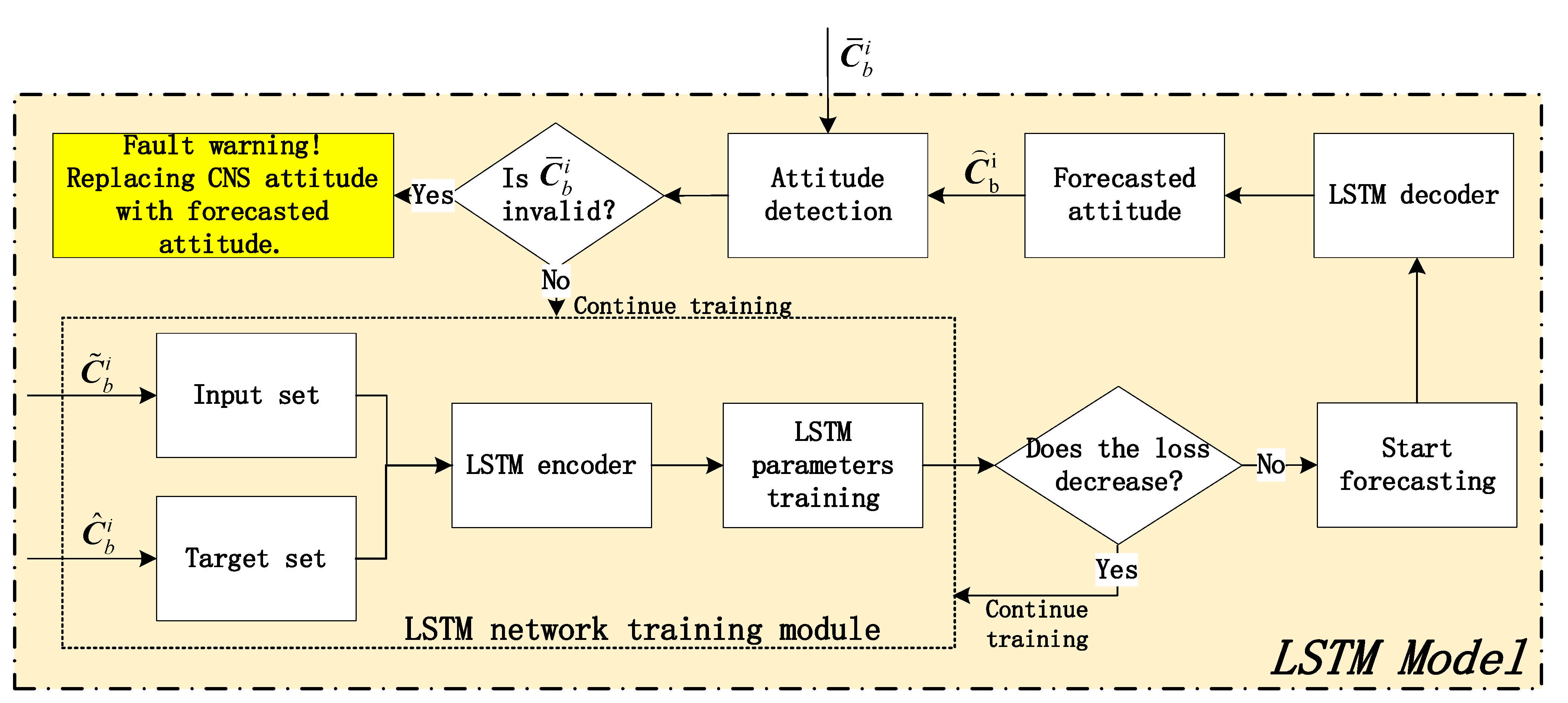
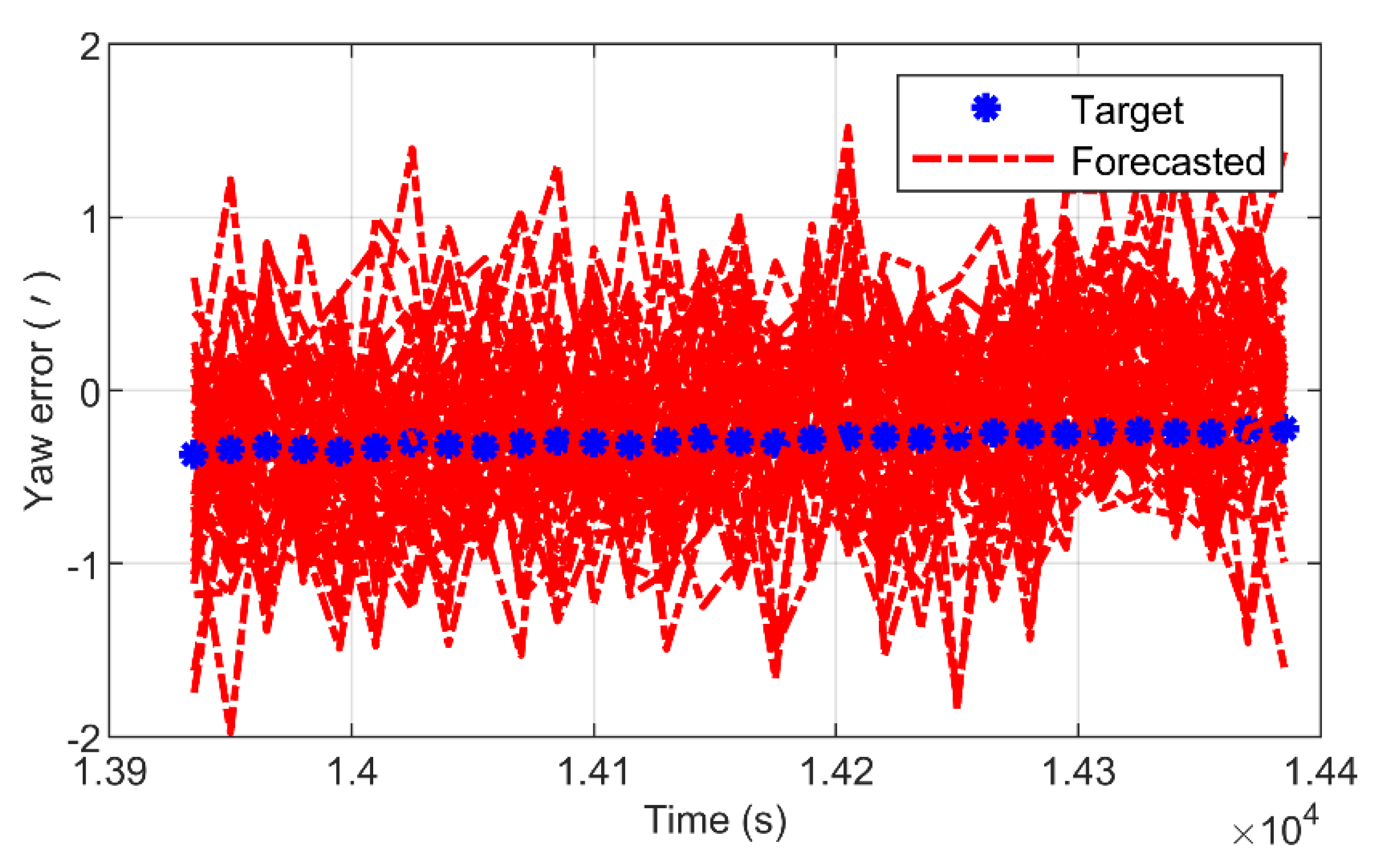
The diagram of the technical framework for the LSTM attitude forecast model is summarized in Figure 1. The input set is constructed by the attitude ${\tilde{\mathit{C}}}_b^i$ output from the SINS independent solution module. The target set is constructed by the attitude ${\widehat{\mathit{C}}}_b^i$ output from the SINS/CNS integrated module. The input and target sets are processed by the LSTM encoder to be converted to a data type suitable for the LSTM model training. Then, the LSTM begins learning to determine the hyperparameters and model parameters through iterative training. If the loss continues to decrease, the training continues; otherwise, the forecast starts. The forecasted result is converted to attitude ${\stackrel{⌢}{\mathit{C}}}_b^i$ by the LSTM decoder. With the forecasted attitude as a reference, the attitude ${\overline{\mathit{C}}}_b^i$ is detected from the CNS module. If the attitude ${\overline{\mathit{C}}}_b^i$ is invalid, a fault warning is issued and the CNS attitude ${\overline{\mathit{C}}}_b^i$ will be replaced with the LSTM forecasted attitude ${\stackrel{⌢}{\mathit{C}}}_b^i$ for information fusion with the SINS; otherwise, the training continues.

Remark 2. 

In the practice of LSTM model training, the input attitude, the target attitude and the forecasted attitude are all constructed in the form of three-dimensional Euler angles, but in order to facilitate understanding and expression, the attitude is described in the form of a matrix in this article.

3.1. Selection of Input Set and Target Set

The target set refers to the dataset composed of the parameters used as the forecasted target, and the input set refers to the dataset composed of the parameters that can accurately and fully reflect the features of the target. Obviously, the selection of input is determined by the target; whether the input matches the target is the key factor affecting the forecasted performance of the LSTM network.

According to the theory of optimal estimation, the precision of navigation parameters after information fusion with integrated navigation is better than that of each subsystem. Therefore, the attitude ${\widehat{\mathit{C}}}_b^i$ output from the SINS/CNS is selected to construct the target set. The input should not only reflect the attributes of the target attitude, but also have the anti-interference ability without the influence of CNS rejection. Consequently, the SINS independent solution module is added into the SINS/CNS integrated navigation system, and the attitude ${\tilde{\mathit{C}}}_b^i$ output from this module is selected to construct the input set.

3.2. LSTM Encoder Based on Seq2Seq

The function of the LSTM encoder is to reassemble, segment and normalize the datasets and make them suitable for network training [21]. According to the different constructures of the input and target, the LSTM time series task can be classified as one-to-one, one-to-many, many-to-one and many-to-many [22]. In order to give full play to the advantage of LSTM in processing the long-term sequence, the data structure of Seq2Seq (many-to-many) is used to construct the LSTM encoder.

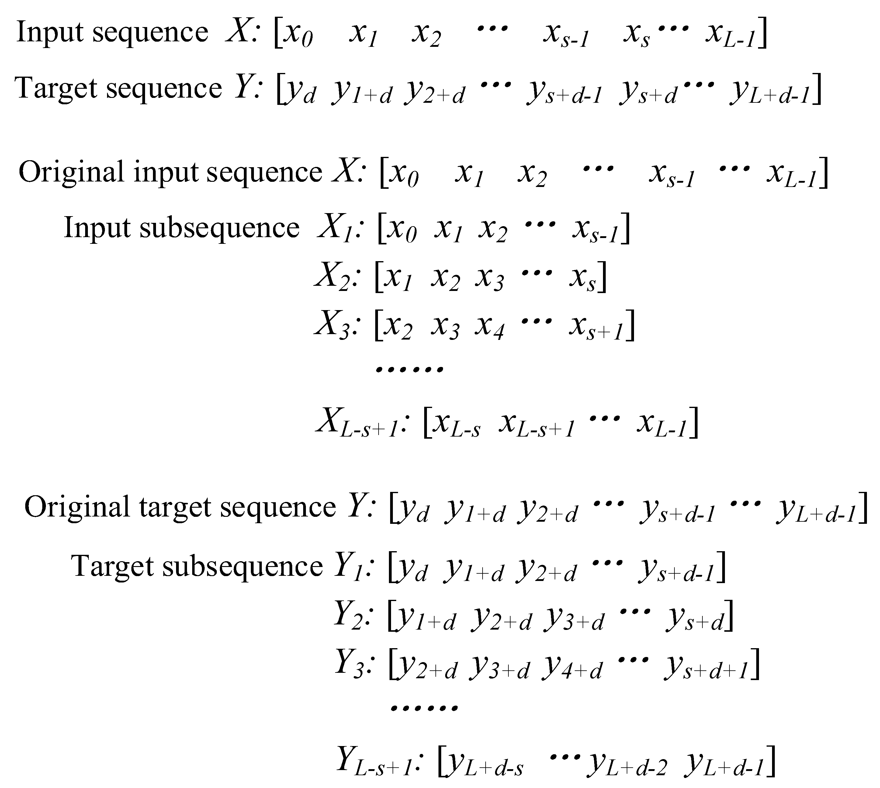
The method of the second-order overlapping shift is proposed to encode the dataset in this article. The first order means that the target sequence is aligned with the input sequence in the form of an overlapping shift, where the shift step is just the forecasted step (delay). The other order means that the input sequence $X$ and the target sequence $Y$ are divided into a series of subsequences in the form of overlapping shifts.

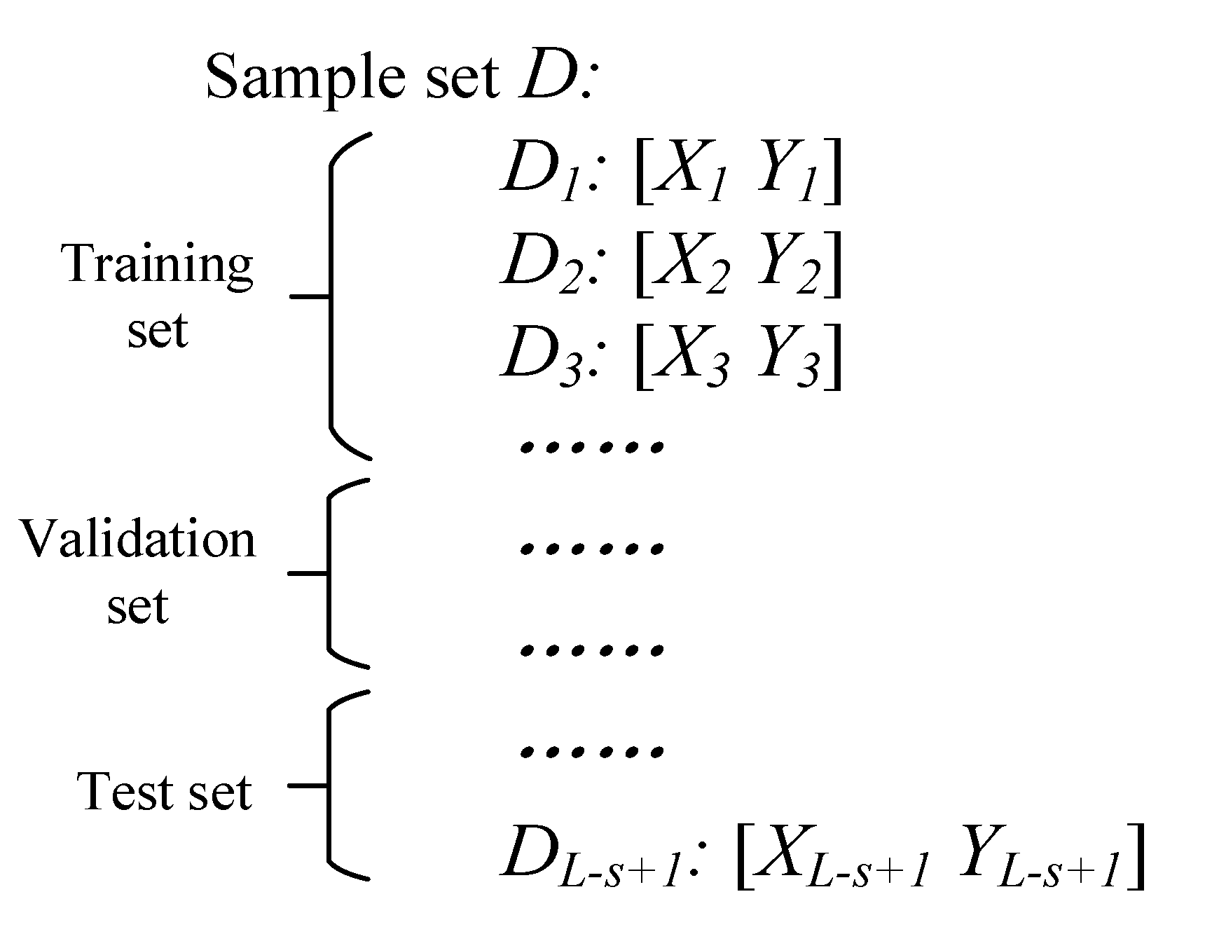
As shown in Figure 2, L is the length of the input and target sequences, s is the length of the input and target subsequences and d is the forecasted step. With s as the sliding window and 1 as the sliding step, the original input and target sequences are divided into L-s + 1 subsequences, respectively. On this basis, a sample $D$ set is constructed with L-s + 1 samples, as shown in Figure 3. The sample set $D$ is divided into a training set, a validation set and a test set according to a certain ratio (usually 6:2:2, 7:2:1 or 8:1:1).

3.3. Bayesian Hyperparameter Optimization

The performance of a deep learning model is mainly determined by two types of parameters, model parameters and model hyperparameters. Model parameters are a set of internal parameters used to determine a deep learning model, such as the weight coefficient matrix and the bias vector in the various gate structures of the LSTM neural network. Hyperparameters are a set of external parameters used to design the network structure and training strategy to optimize the training effect of the model. Model parameters can be obtained independently with deep learning for sample $D$ without manual intervention. However, the learning of the model parameters is directly affected by the hyperparameters, so the focus is on the problem of hyperparameter optimization as follows.

According to the application characteristics of the ship attitude forecast, the loss function based on the algorithm of mean squared error (MSE) is used as the objective function for hyperparameter optimization.

$$loss\left(x=x_k\right)=1/n\sum _{i=1}^n{(y_i-{\widehat{y}}_i)}^2$$

(10)

where $x_k$ represents a set of hyperparameter sampling values, $y_i$ represents the target attitude in the validation set, ${\widehat{y}}_i$ represents the forecasted attitude and $n$ is the number of samples. Hyperparameter optimization aims to find a set of ideal hyperparameters to minimize the objective function. This process can also be simply considered as finding a set of hyperparameters $x^{*}$ to minimize the attitude forecast error of the LSTM model, as shown in (11).

$$x^{*}=arcmin loss\left(x\right), x\in X$$

(11)

where $X$ is the value range of the hyperparameters to be optimized.

At present, Bayesian optimization has been applied more and more widely in solving the black box function and has become the mainstream method for hyperparameter optimization [30]. Bayesian hyperparameter optimization mainly consists of two technical modules, a learning surrogate model and constructing an acquisition function [31].

3.3.1. Learning Surrogate Model

The objective function belongs to the black box function. It is difficult to obtain the function’s specific expression, and the calculation cost is expensive. Therefore, Bayesian optimization must first choose a surrogate model for the objective function. The Gaussian process regression (GPR) model is a widely used and efficient surrogate model. On the basis of assuming that the objective function conforms to the Gaussian distribution, the mathematical expectation ${\mu }_0\left(x_{1:k}\right)$ and covariance matrix ${\sigma }_0\left(x_{1:k},x_{1:k}\right)$ are calculated by sampling the input and output k times, and then a Gaussian process regression model $g\left(x\right)$ is trained to replace the objective function $loss\left(x\right)$. $g\left(x\right)$ satisfies the following Gaussian process (GP):

$$g\left(x\right)~GP({\mu }_0\left(x_{1:k}\right), {\sigma }_0\left(x_{1:k},x_{1:k}\right))$$

(12)

where

$${\mu }_0\left(x_{1:k}\right)={[{\mu }_0\left(x_1\right),{\mu }_0\left(x_2\right),\cdots {\mu }_0\left(x_k\right)]}^T$$

(13)

$${\sigma }_0\left(x_{1:k},x_{1:k}\right)=\left[\begin{array}{ccc}{\sigma }_0\left(x_1,x_1\right)& \cdots & {\sigma }_0\left(x_1,x_k\right)\\ ⋮& \ddots & ⋮\\ {\sigma }_0\left(x_k,x_1\right)& \cdots & {\sigma }_0\left(x_k,x_k\right)\end{array}\right]$$

(14)

3.3.2. Constructing Acquisition Function

In order toget the approximate global optimal value of the objective function as soon as possible, it is necessary to construct the acquisition function $a\left(x|D_n\right)$ to select the next sampling point $x_{n+1}$ (that is, another set of hyperparameters) optimally, where $D_n$ is expressed as

$$D_n=D_0\cup \{x_{1:n},loss\left(x_{1:n}\right)\}$$

(15)

$$D_0=\{x_{1:k},loss\left(x_{1:k}\right)\}$$

(16)

where $x_{1:k}$ represents the k sampling points that are used to initialize the surrogate model and $loss\left(x_{1:k}\right)$ represents the loss values corresponding to $x_{1:k}$. $x_{1:n}$ represents another n sampling points after $x_{1:k}$ and $loss\left(x_{1:n}\right)$ represents the loss values corresponding to $x_{1:n}$. The surrogate model will continue to learn and update with the subsequent sampling, so the acquisition function $a\left(x|D_n\right)$ can also be considered as the distribution of sampling points based on the given surrogate model, and satisfies

$$a\left(x|D_n\right)~GP({\mu }_n,{\sigma }_n^2)$$

(17)

$${\mu }_n=f(x_{1:n},loss\left(x_{1:n}\right),{\mu }_0\left(x_{1:k}\right))$$

(18)

$${\sigma }_n^2=m(x_{1:n},{\sigma }_0\left(x_{1:k},x_{1:k}\right))$$

(19)

where $f\left(\right)$ and $m\left(\right)$ are the calculated functions for the mathematical expectation ${\mu }_n$ and covariance matrix ${\sigma }_n^2$, respectively [32]. Because the explicit expressions of the two functions are relatively complicated, and they can be directly calculated by the Bayesian optimization library, this article does not expand the description.

The expected improvement (EI) model is used to construct the acquisition function. To define the improvement of sampling points

$$I\left(x_{1:q}\right)=max(loss\left(x^{*}\right)-loss\left(x_{1:q}\right),0)$$

(20)

where $loss\left(x^{*}\right)$ is the approximate optimal solution of the objective function after the sampling points $x_{1:n}$. $x_{1:q}$ represents the value space of the next sampling point near $x^{*}$. If $loss\left(x_{1:q}\right)$ is smaller than $loss\left(x^{*}\right)$,return the descent degree; otherwise, return 0. Following this law, the acquisition function is constructed as

$$a\left(x_{1:q}|D_n\right)=E\left(I\right(x_{1:q}\left)\right)$$

(21)

where $E\left(I\right(x_{1:q}\left)\right)$ represents the mathematical expectation of $I\left(x_{1:q}\right)$. The probability distribution of $a\left(x|D_n\right)$ can be determined by (17)–(19), so $x_{n+1}$ is the next sampling point that maximizes the EI of the acquisition function, that is

$$x_{n+1}=argmax a\left(x|D_n\right), x\in x_{1:q}$$

(22)

3.3.3. Bayesian Hyperparameter Optimization Algorithm

To sum up, Bayesian hyperparameter optimization can be summarized as Algorithm 1.

Algorithm 1: Bayesian hyperparameter optimization
	$\mathrm{Input}: \mathrm{Initial} \mathrm{sampling} \mathrm{number} k, \mathrm{trial} \mathrm{number} N$, selecting surrogate model (GPR) and acquisition function
	$\mathrm{Output}: \{x^{\mathrm{*}},loss\left(x^{\mathrm{*}}\right)$}
1	Begin
2	$\hspace{1em}\mathrm{Step} 1: \mathrm{Selecting} \mathrm{sampling} \mathrm{points} x_{1:k} \mathrm{randomly} \mathrm{to} \mathrm{calculate} loss\left(x_{1:k}\right)$
3	$\hspace{1em}\mathrm{Step} 2: \mathrm{Constructing} \mathrm{initial} \mathrm{set} D_0=\left\{x_{1:k},loss\left(x_{1:k}\right)\right\}, \mathrm{let} n=k, D_n=D_0$
4	$\hspace{1em} \mathrm{While} n<N\hspace{1em}$ do
5	$\hspace{1em}\hspace{1em}\mathrm{Step} 3: \mathrm{According} \mathrm{to} D_n, \mathrm{training} \mathrm{surrogate} \mathrm{model} g\left(x\right)$
6	$\hspace{1em}\hspace{1em}\mathrm{Step} 4: \mathrm{According} \mathrm{to} \mathrm{the} \mathrm{current} g\left(x\right), \mathrm{determining} \mathrm{the} \mathrm{distribution} \mathrm{of} \mathrm{acquisition} \mathrm{function} a\left(x|D_n\right)\mathrm{to} \mathrm{obtain} x_{n+1}=argmaxa\left(x|D_n\right)$
7	$\hspace{1em}\hspace{1em}\mathrm{Step} 5: \mathrm{According} \mathrm{to} x_{n+1}, \mathrm{calculating} loss\left(x_{n+1}\right), \mathrm{then} \mathrm{updating} D_n: D_n=D_n\cup \left\{x_{n+1},loss\left(x_{n+1}\right)\right\}$
8	End
9	$\hspace{1em} \mathrm{Output}: \{x^{\mathrm{*}},loss\left(x^{\mathrm{*}}\right)$}
10	End

3.4. Training for LSTM Model

The training for the LSTM model can be summarized as Algorithm 2.

Algorithm 2: Training for LSTM model
	$\mathrm{Input}: \mathrm{Training} \mathrm{epoch} \mathrm{number} n\_epochs, \mathrm{early} \mathrm{stop} \mathrm{count} i, \mathrm{training} \mathrm{set} D_{tra}, \mathrm{validation} \mathrm{set} D_{val}$
	Output: LSTM model
1	Begin
2	Step 1: Initializing the default hyperparameters, setting the value space for the hyperparameters to be optimized
3	Step 2: Instantiating LSTM model
4	$\hspace{1em} \mathrm{While} epoch<n\_epochs$ do
5	$\hspace{1em}\hspace{1em} \mathrm{Step} 3: \mathrm{According} \mathrm{to} D_{tra}, \mathrm{training} \mathrm{and} \mathrm{updating} \mathrm{surrogate} \mathrm{model} g\left(x\right)$
6	$\hspace{1em}\hspace{1em} \mathrm{Step} 4: \mathrm{According} \mathrm{to} D_{val}, \mathrm{calculating} {loss}_{val}$
7	$\hspace{1em}\hspace{1em} \mathrm{If} {loss}_{val} \mathrm{does} \mathrm{not} \mathrm{decrease} \mathrm{in} \mathrm{consecutive} i$ epochs of training
8	$\hspace{1em}\hspace{1em}\hspace{1em}\mathrm{break}, (\mathrm{go} \mathrm{to} \mathrm{line} 11, \mathrm{output} \mathrm{the} \mathrm{current} \mathrm{LSTM} \mathrm{model} \mathrm{and} {loss}_{val}$)
9	End
10	End
11	$\hspace{1em} \mathrm{Output}: \mathrm{LSTM} \mathrm{model}, {loss}_{val}$
12	End

In fact, the core target of the LSTM model training can be understood as the process of determining the model hyperparameters and model parameters based on the training set and validation set with the loss function as the evaluation index. As mentioned above, Algorithm 2 “training for LSTM model” is closely related to Algorithm 1 “Bayesian hyperparameter optimization”. In practical applications, Algorithm 2 is often nested in Algorithm 1. One of output of Algorithm 2, ${loss}_{val}$, is just the $loss\left(x_{1:k}\right)$ in Algorithm 1.

4. Results and Discussion

The LSTM attitude forecast model is established based on the learning of the actual attitude change law of ships, and it works under the supervision of the attitude independently solved by the SINS. Due to the requirements of the relevant policies and confidentiality agreements, the marine observation data of the CNS cannot be disclosed. Therefore, we simulated a ship’s attitude changes at sea through a mathematical model to conduct the experiments for the LSTM attitude forecast and SINS/CNS integrated navigation.

4.1. Experiment Preparation

It is assumed that three stars need to be observed for each celestial navigation solution, and the observed azimuth angle and altitude angle for each star are randomly assigned within the ranges listed in

Table 1. Observations of stars.

Star	Rang of Azimuth Angle	Rang of Altitude Angle
$S_1^b$	[80°, 100°]	[30°, 60°]
$S_2^b$	[−40°, −20°]	[30°, 60°]
$S_3^b$	[−160°, −140°]	[30°, 60°]

.

The projections of the observed stars in inertial frame i can be obtained by

$${\mathit{S}}_j^i={\mathit{C}}_e^i{\mathit{C}}_n^e{\mathit{C}}_b^n{\mathit{S}}_i^b, i=1,2,3$$

(23)

The performance indexes of the sensors in simulation are listed in

Table 2. Performance index of the sensors.

Sensor	Parameter	Index
SINS	Gyro drift	$0.03°/\mathrm{h}$
	Gyro random noise	$0.001°/\sqrt{\mathrm{h}}$
	Accelerometer bias	$100 \mathsf{\mu }\mathrm{g}$
	Accelerometer noise	$5 \mathsf{\mu }\mathrm{g}/\mathrm{H}\mathrm{z}$
	Data update frequency	$100 \mathrm{H}\mathrm{z}$
CNS	Measurement noise [azimuth, altitude]	$[{20}^{″},{10}^{″}]$
	Observation time for single star	5 s

.

The initial parameters for simulation are listed in

Table 3. The initial parameters.

Parameter	Initial Value
Initial attitude	$[0°,0°,60°]$
Initial velocity	$[0.5 \mathrm{m}/\mathrm{s},0.5 \mathrm{m}/\mathrm{s},0 \mathrm{m}/\mathrm{s}]$
Initial position	$(30.394491° \mathrm{N},114.345490° \mathrm{E})$
Initial attitude variance	${[1^{\prime },1^{\prime },{10}^{\prime }]}^2$
Initial velocity variance	${[0.1 \mathrm{m}/\mathrm{s},0.1 \mathrm{m}/\mathrm{s},0.1 \mathrm{m}/\mathrm{s}]}^2$
Initial position variance	${[1 \mathrm{m},1 \mathrm{m},1 \mathrm{m}]}^2$
$\mathrm{Attitude} \mathrm{changing} \mathrm{amplitude} A$	$[3°,4°,2°]$
Attitude changing period $T$	$[20 \mathrm{s},20 \mathrm{s},18 \mathrm{s}]$
$\mathrm{Attitude} \mathrm{initial} \mathrm{phase} P$	$[0,\pi /6,0]$

.

The changes in the ship’s three-dimensional attitude $[pithch \theta ,roll \gamma ,yaw \psi ]$ are simulated as

$$\theta =A_{\theta }\sin \left(\right(2\pi /T_{\theta })t+P_{\theta })$$

(24)

$$\gamma =A_{\gamma }\mathit{sin}\left(\right(2\pi /T_{\gamma })t+P_{\gamma })$$

(25)

$$\psi =A_{\psi }\mathit{sin}\left(\right(2\pi /T_{\psi })t+P_{\psi })$$

(26)

where the amplitude $A$, period $T$ and initial phase $P$ have been listed in Table 3.

The attitude errors calculated by SINS/CNS integrated navigation are shown in Figure 4.

Remark 3. 

Since the simulation time is as long as 4 h (14,400 s), the attitude curves along the time axis are too dense to be distinguished; they are not presented in this article.

According to the method described in Section 3.3, the hyperparameters to be optimized and their optimized results are listed in

Table 4. The hyperparameters to be optimized.

Parameter	Value Spaces	Optimized Results
Learning rate	$[1\times {10}^{-5} :1\times {10}^{-2}]$	$4.31\times {10}^{-3}$
Sequence length	$[17, 47, 77, 107]$	107
Number of layers	$[1, 2, 3, 4]$	1
Hidden size	$[64, 128, 256, 512]$	512
Optimizer	$[\mathrm{A}\mathrm{d}\mathrm{a}\mathrm{m},\mathrm{R}\mathrm{M}\mathrm{S}\mathrm{p}\mathrm{r}\mathrm{o}\mathrm{p},\mathrm{S}\mathrm{G}\mathrm{D}]$	$\mathrm{A}\mathrm{d}\mathrm{a}\mathrm{m}$

.

Remark 4. 

Adam (Adaptive Moment Estimation) is a gradient descent algorithm for training neural networks. It combines the momentum algorithm and the adaptive learning rate algorithm to achieve faster convergence and better generalization ability by calculating different adaptive learning rates for each model parameter. In this article, Adam is used to train the weights and the biases of the LSTM. The LSTM model is trained using PyCharm 2021.3.1 with the help of the machine learning library of PyTorch 2.2.0, and the simulation program is implemented using Matlable (https://ww2.mathworks.cn/en/products/matlab.html, accessed on 1 February 2023).

4.2. Attitude Forecast

We use the trained LSTM model to forecast the attitude of the SINS/CNS during a period of 13,935 s–14,385 s (450 s). The observation time for each star is 5 s, and it will take 15 s to observe three stars to complete one celestial navigation solution. Therefore, a time series forecast of 30 steps will be performed in 450 s with the single step interval of 15 s. Since the change in the ship’s attitude is much greater than the attitude forecasted error, it is difficult for the attitude tracking curve to distinguish the target attitude from the forecasted attitude. Therefore, the attitude error curve is used to show the forecasted accuracy in Figure 5, Figure 6 and Figure 7.

To make the results more convincing, 50 Monte Carlo simulation experiments are conducted to evaluate the performance of the LSTM forecast model. The root mean square error (RMSE) is used as a performance metric to quantitatively analyze the forecasted error, and the RMSE of the Monte Carlo simulations is shown in

Table 5. RMSE of the forecasted attitude.

Pitch (′)	Roll (′)	Yaw (′)
0.42	0.45	0.57

.

The RMSE of the forecasted pitch and roll are less than 0.5′, and that of the forecasted yaw is less than 0.6′. Although SINS/CNS integrated navigation can effectively suppress the divergence of yaw error, the input of the LSTM model is the attitude independently solved by the SINS, whose yaw error diverges with time, and the forecasted target corresponding to this dimension feature is the yaw provided by SINS/CSN integrated navigation. Therefore, the mapping relationship between the input and output of the yaw is more complicated than that of the pitch or roll, and the forecasted error is also relatively larger. In addition, as can be seen from Figure 5, Figure 6 and Figure 7, the forecasted results tend to gradually deviate from the target value over time. This is because that although LSTM has excellent forecasting ability for long time series, the forecasted steps are still limited, as its name, “long short-term memory”, indicates. With the increase in forecasted steps, the reliability of the historical information will gradually weaken, and more and more data excluded in training set will enter into the model, which will result in a larger forecasted error.

4.3. SINS/CNS/LSTM Integrated Navigation

In order to verify the auxiliary effect of the LSTM model on SINS/CNS integrated navigation, the experiment is designed as follows. At a time of 13,935 s in the simulation experiment, 100 times the observation noise (CNS observation noise is shown in Table 2) was injected into the observed star, which led to an abnormal observation value, and then the CNS signal was interrupted.

The experimental results are shown in Figure 8, Figure 9 and Figure 10, where the blue curve is the attitude error of SINS/CNS integrated navigation during the CNS normal operation. The yellow curve is the attitude error of the SINS independently solved, after the CNS observation is abnormal and interrupted. The red curve is the attitude error of the SINS/LSTM information fusion, after the CNS observation is abnormal and interrupted. Due to the abnormal observation of the CNS, the attitude error changes instantaneously and diverges rapidly with the time update of the SINS. However, the SINS/LSTM information fusion still maintains the propagation trend of the attitude error, which is basically the same as that of SINS/CNS integrated navigation.

5. Conclusions

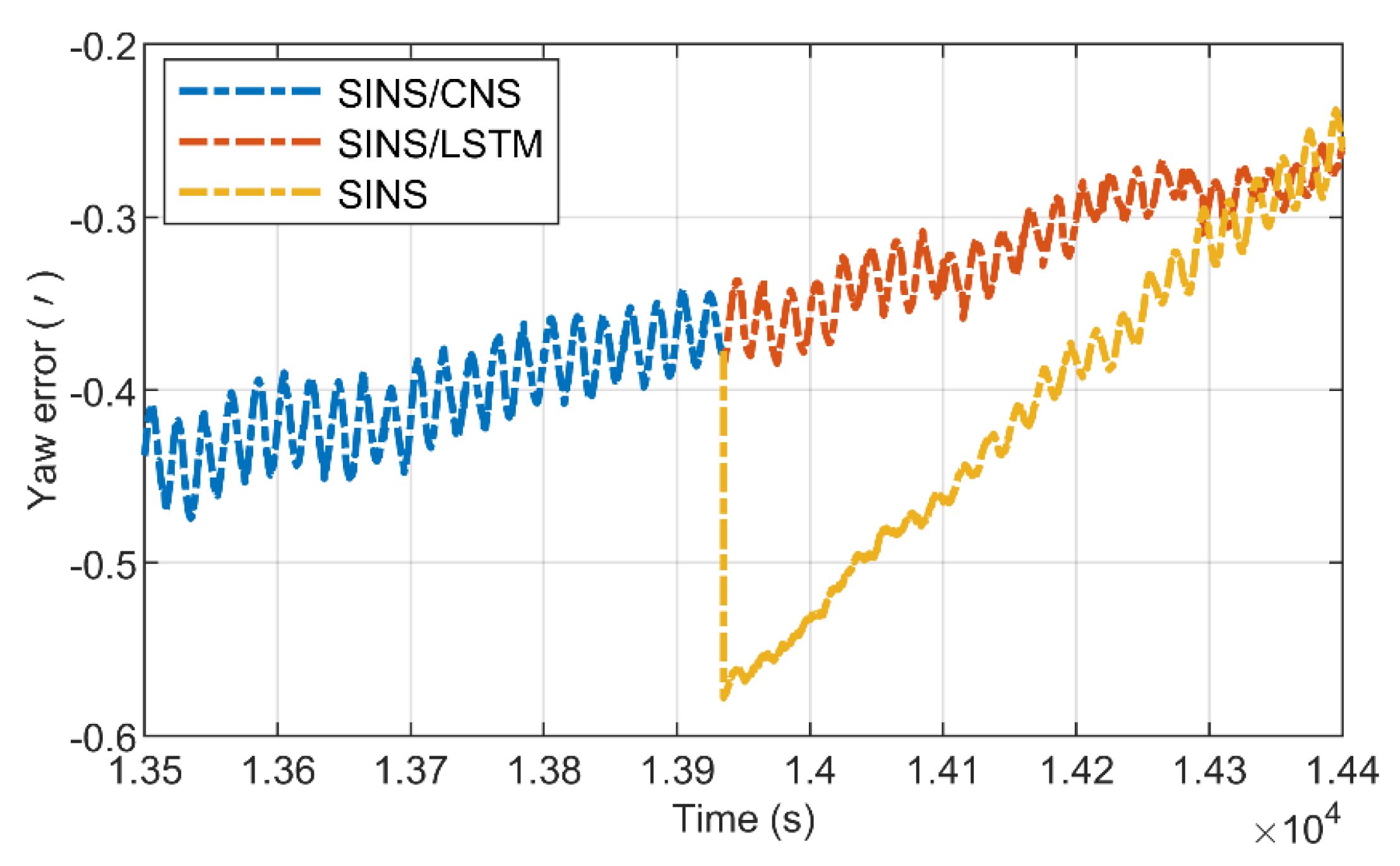
This article presented a complete set of technical solutions for ship SINS/CNS integrated navigation aided by LSTM-RNN. The LSTM model accomplished a high-precision attitude forecast for ships. In the case of CNS signal abnormality or even failure, the LSTM forecasted attitude is used as reference information fused with the SINS, which has ensured the continuous and stable output of high-precision navigation information, expanded the application boundary of ship SINS/CNS integrated navigation and effectively improved the robustness of the integrated system.

Compared with the traditional SINS/CNS integrated navigation method, although the technical scheme proposed in this paper increases the computational load of the system through the optimized design of the LSTM network structure and training strategy, the mapping relationship between the input and output of the forecasted model is much simpler. With the support of the integrated computing environment, the increased computational burden is completely acceptable. In addition, in our future research, we will study more accurate and efficient SINS/CNS integrated navigation models that are more suitable for deep learning algorithms.