Article

Research on Three-Closed-Loop ADRC Position Compensation Strategy Based on Winch-Type Heave Compensation System with a Secondary Component

1
Institute of Marine Science and Technology, Shandong University, Jinan 250061, China
2
Taiyuan Heavy Machinery Group Yuci Hydraulic Industry (Jinan) Co., Ltd., Jinan 250104, China
3
Cnooc Energy Logistics Co., Ltd., Tianjin 300452, China
*
Author to whom correspondence should be addressed.
J. Mar. Sci. Eng. 2024, 12(2), 346; https://doi.org/10.3390/jmse12020346
Submission received: 16 January 2024 / Revised: 5 February 2024 / Accepted: 10 February 2024 / Published: 17 February 2024
(This article belongs to the Section Ocean Engineering)

Abstract

:
To mitigate the interference of waves on an offshore operation ship, heave compensation systems find widespread application. The performance of heave compensation systems significantly influences the efficiency and safety of maritime operations. This study established a mathematical model for a winch-based active heave compensation system. It introduced a three-loop active disturbance rejection control (ADRC) strategy that encompasses piston position control, winch speed control, and load-displacement control to enable the real-time estimation and compensation of system disturbances, thereby enhancing the performance of the heave compensation system. To assess the effectiveness of this control strategy, this study employed Matlab/Simulink and AMESim to construct a co-simulation model and conducted a comparative analysis with traditional proportional integral derivative (PID) control systems. The research findings indicate that the three-loop ADRC position control strategy consistently delivered superior compensation performance across various operational scenarios.

Graphical Abstract

1. Introduction

With the increasing scope and demand for ocean exploration, there is a growing demand for offshore engineering equipment. The active heave compensation (AHC) system can be used to correct and compensate for the heave motion in the vertical direction that occurs during the offshore operations of a vessel [1]. Applying this technology effectively avoids issues such as severe load motion, inaccurate positioning, wire rope breakage, and risks to the safety of personnel, thereby greatly improving the efficiency and safety of marine operations [2]. An actively controlled heave compensation system consisting of a hydraulic transmission mechanism and a winch actuation mechanism has a wide range of applications. This type of active compensation system has the advantages of being suitable for compensation in a wide range of sea conditions and high compensation accuracy. However, its disadvantages include a complex system structure, heavy reliance on the controller for compensation effectiveness, the requirement of an additional power source for the system itself, and high energy consumption [3].
To improve the performance of the active compensation system, scholars and companies from various countries have conducted research in areas such as mechanical structural design, control strategies, and numerical simulations [4,5,6]. Dabing et al. introduced a technology called a secondary control hydraulic drive into the offshore crane system [7]. The secondary components can absorb the potential energy of the effective payload under pump conditions and convert the mechanical energy into hydraulic energy stored in an accumulator to save energy. Bosch Rexroth introduced new types of hydraulic axial piston pumps, namely, the A4VSO and A4VSG, combined with a new secondary control HNC controller [8]. The system gives full consideration to the special characteristics of the use of the environment, drives the marine lifting winch for positive and negative rotation so that the suspended weight can remain relatively static, ensures that the equipment is stable and reliable when working at sea, and better meets the needs of practical applications. A company Royal IHC from the Netherlands developed an active heavy compensation system [9]. This system utilizes a winch structure and can control the constant tension of the wire rope during lifting operations. The active compensation system has a compact size and improved control performance, showcasing its superiority in certain low-power conditions. However, its drawback is that it consumes a large amount of power, limiting its application in high-power working situations. Moslått integrated National Oilwell Varco’s wave compensation crane and motor feedforward control technology to propose a hybrid active–passive heave compensation system [10]. This system demonstrates strong adaptability and flexibility.
To achieve high-precision compensation, effective control system schemes can be designed and appropriate control strategies can be selected [11]. There are many methods for traditional heave compensation system control, such as proportional integral derivative control (PID), sliding mode control (SMC), and model predictive control (MPC) [12,13,14]. Using ordinary traditional controllers for complex nonlinear systems cannot achieve satisfactory control performance and accuracy [15]. In practical work, the AHC system is affected by external disturbances, including friction, clear dynamic models, changes in effective payload weight, and parameter uncertainties.
Do and Pan first studied the nonlinear controller of AHC systems [16]. They designed a disturbance observer for the active heave compensation system in the electro-hydraulic system, which improved the control performance of the active heave compensation system. Küchler and Sawodny proposed a nonlinear control method consisting of feedforward and stable controllers to directly control the hydraulic drive winch of offshore cranes, decouple the load’s motion from the one of the ship, and achieve trajectory tracking of the payload in the coordinate system [17]. The application of improved forms of traditional control methods is increasing. Hexiong Zhou proposed a robust hierarchical control scheme for a hydraulic-driven winch-based AHC system based on the combination of a nonlinear model predictive control (NMPC) strategy to alleviate the negative impact of the support vessels’ vertical heave motion on the station-keeping and position-tracking performance [18]. Zhang Q. proposed a PID-DDPG hybrid control method to improve the heave compensation efficiency [19]. The simulation results show that the proposed hybrid control method has the highest compensation efficiency compared with PID and DDPG under different sea conditions.
Quadrotors have stricter requirements for control strategies, which can be inspired by the study of the control strategies used in quadcopters. In order to track the trajectories of quadcopters in the presence of disturbances and model uncertainties, a new filtered observer-based interconnection and damping assignment productivity-based control (IDA-PBC) strategy was developed by Guerrero-Sanchez and Hernandez-Gonzalez et al. [20]. Najafi and Vu et al. proposed an adaptive barrier fast terminal sliding mode control (ABFTSMC) approach for quadrotor unmanned aerial vehicles (UAVs) [21]. Zhou R. and Neusypin K. proposed a cascade ADRC control scheme for fixed-wing UAVs and tested the proposed control scheme through a series of simulations [22]. Deng B. and Xu J. proposed a trajectory-tracking control system based on the ADRC for the compound unmanned aircraft to adapt the full flight modes [23]. Its control structure is very similar to the control of the heave compensation system.
Active disturbance rejection control (ADRC) can observe disturbances, which endows it with high robustness and the advantage of not depending on system models. This allows it to enhance the effectiveness of compensation and the ability to resist interferences [24,25]. As a result, ADRC is widely applied in various control systems. Messineo and Serrani proposed an adaptive controller for large offshore crane operations, relying on the use of an adaptive observer and two adaptive disturbance external models [26]. This controller effectively reduces the hydrodynamic impact load when the load enters the water. Li et al. applied the disturbance-attenuation-based ADRC, which is independent of mathematical models and has strong anti-interference capability to provide tension control for heave compensation [27]. A newly developed second-order ADRC controller is used in the tension control strategy, leading to an improved compensation effect.
In this study, the authors conducted research on the design and control of winch-based active heave compensation. They introduced a secondary component and ADRC [28,29], then proposed a three-closed-loop ADRC position compensation strategy based on a secondary component to resist external disturbances, which, in turn, improved the accuracy of the heave compensation system. The inner loop is the piston displacement control loop of the variable control cylinder, the middle loop is the winch rotation speed control loop, and the outermost loop is the load-displacement control loop. By properly setting the parameters of each ADRC loop, good control effects on the load displacement could be achieved. Finally, a joint simulation model was established using Matlab/Simulink R2020a and AMESim 2019.1, and a comparative analysis was performed with a PID control system to verify the proposed three-closed-loop ADRC position compensation strategy based on a winch-type heave compensation system with a secondary component.
The control strategy proposed in this paper does not rely on the system model, making it convenient to design and it demonstrate good performance. The rest of this paper is organized as follows. Section 2 introduces the composition of the heave compensation system structure and the establishment of the mathematical model. Section 3 presents the principles, design process, and stability proof of the ADRC controller. Section 4 discusses the performance comparison between the controller designed in this paper and the PID controller under three scenarios: step response, sine disturbance, and actual sea conditions. The conclusion is provided in Section 5. The end and Appendix A of the article are tables of nomenclature/abbreviations and variable explanations

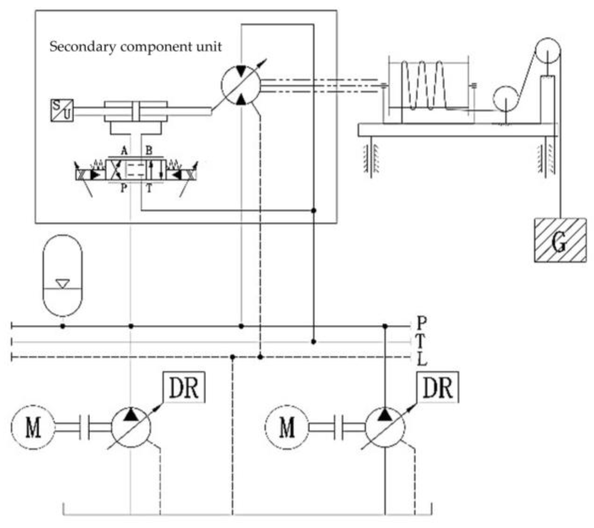
2. Dynamic Model of Heave Compensation System

The schematic diagram of a winch-type heave compensation system based on a secondary component is shown in Figure 1. The system consists of secondary components, a constant-pressure oil source, a cable-winding winch, variable control oil cylinders, and other modules. The utilization of secondary control techniques achieves significant energy recovery. This is mainly because the secondary component can switch between the operating conditions of a pump and a motor. When the output torque of the secondary component is greater than the load gravity, it operates in the motor condition, driving the load to rise and consuming energy. When the load gravity is greater than the output torque of the secondary component, it operates in the pump condition. The load drives the rotation of the secondary component, converting gravitational potential energy into hydraulic energy and storing it in the accumulator to achieve energy recovery.

2.1. Mathematical Modeling

The heave compensation system is mainly controlled through electro-hydraulic servo valves, variable control oil cylinders, secondary components, and a cable winding system. The displacement of the variable control oil cylinder piston is controlled by the electro-hydraulic servo valve, which, in turn, regulates hydraulic flow. The secondary component unit operates in a constant-pressure network, resulting in a proportional relationship between its output torque and displacement. By controlling the displacement of the variable control oil cylinder piston, the secondary component achieves variable displacement, thereby adjusting the winch’s output torque. The balance between the load torque and the output torque is maintained through the cable-winding system, which ensures the controlled displacement and speed of the load. The displacement of the variable control oil cylinder piston, winch speed, and load displacement are all regulated by the ADRC controller, with the control structure being a three-closed-loop ADRC position control, as illustrated in Figure 2.

2.1.1. The Model of the Electro-Hydraulic Servo Valve

The mathematical model of the electro-hydraulic servo valve, after simplification, is typically represented is
Q sf s I s = K v s 2 ω n 2 + 2 ξ n ω n s + 1
In this equation, Qsf represents the output flow, I is the coil input current, Kv is the flow gain, s is the Laplace operator, ωn is the natural frequency, and ξn is the damping ratio. Due to its inherent frequency generally being much higher than the system bandwidth, it can be approximated as a proportional link:
Q sf s I s = K v

2.1.2. Variable Control Oil Cylinder

The continuity equation for fluid flow is
q = A g d x g   d t + C t   p + V t 4 β e d p d t
C t = C i + 1 2 C e
In these equations, q is the flow entering the high-pressure chamber of the cylinder, Ag is the effective piston area inside the cylinder, xg is the piston displacement, Ct is the total leakage coefficient, p is the pressure difference between the high-pressure and low-pressure chambers, Vt is the total volume of the two chambers, βe is the volumetric modulus of oil, Ci is the internal leakage coefficient, and Ce is the external leakage coefficient.
Further derivation leads to the force balance equation for the variable control oil cylinder:
A g p = m g d 2 x g d t 2 + B g d x g d t + k g x g + F f g
In the equation, mg represents the total mass of the moving components, Bg is the viscous damping coefficient, kg is the spring stiffness, and Ffg is the resistance force acting on the piston.

2.1.3. Secondary Component Displacement

D e r = D ermax x gmax x g
In this equation, Der represents the displacement, Dermax is the maximum displacement, and xgmax is the maximum displacement of the piston.
The force balance equation for the motor-operating condition is
p s D e r = J e r d 2 θ e r d t 2 + B e r d θ e r d t + M L
The force balance equation for the pump-operating condition is
M L = p s D e r + J e r d 2 θ e r d t 2 + B e r d θ e r d t
In these equations, ps represents the constant pressure of the oil supply, Jer is the rotational inertia converted to the output shaft, θer is the main shaft rotation angle of the secondary component, Ber is the viscous damping coefficient converted to the output shaft, and ML is the external load torque.

2.1.4. Cable-Winding System

The displacement equation of the cable-driven load in the vertical direction is
x l = x l 0 + x h   θ e r i j t R + Δ l
Δ l = Δ l d + Δ l s
In these equations, xl represents the displacement of the load in the vertical direction, xl0 is the initial position of the load, xh is the displacement due to the heave of the ship, ijt is the reduction ratio of the gearbox, R is the radius of the winch drum, Δl is the elongation of the cable, Δld is the dynamic elongation of the cable, and Δls is the static elongation of the cable.
In the air, the kinetic equation for the motion of the load driven by the cable is
M L = R i j t ( m e q g + k l Δ l + C l d Δ l d t + m e q d 2 x l d t 2 )
In this equation, meq represents the equivalent mass of the load and cable, kl is the cable’s elastic coefficient, and Cl is the cable’s damping coefficient.

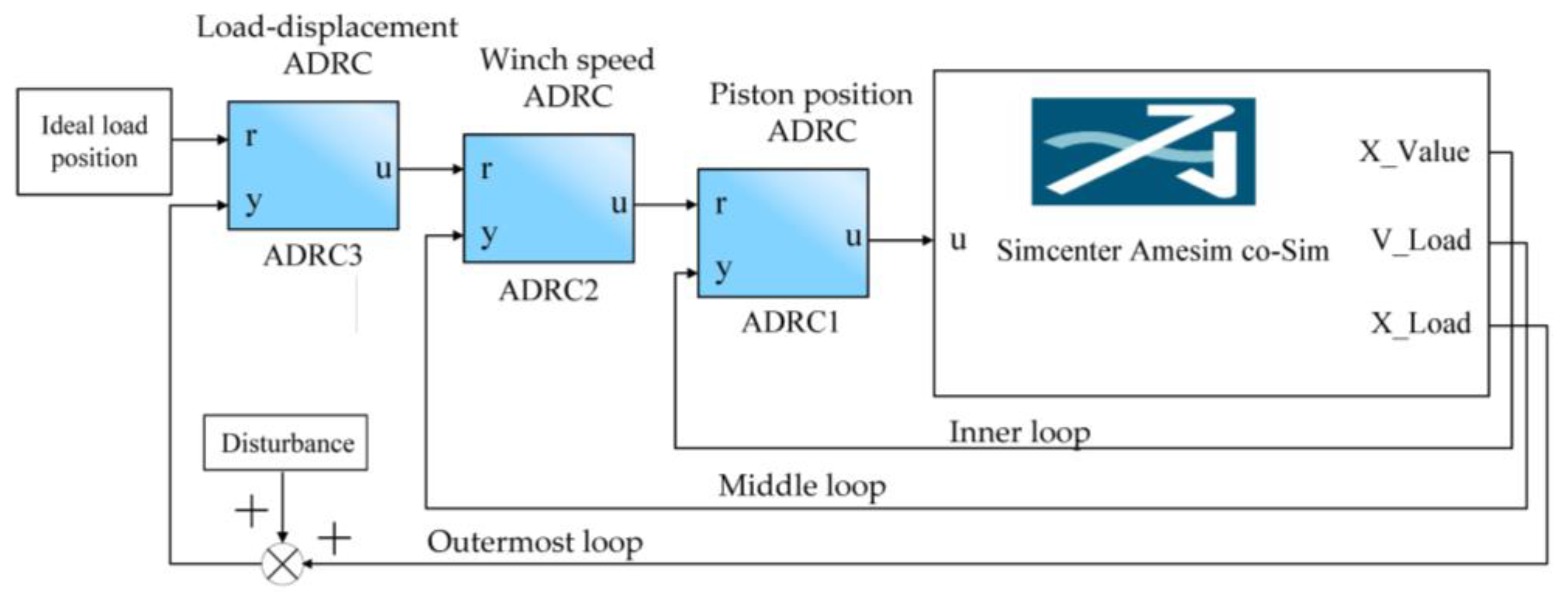
2.2. Simulation Model and Parameter Settings

The control methods applied to practical physical systems must undergo feasibility verification based on computer simulation before being implemented in engineering applications. For the studied winch-type heave compensation system, a combined simulation model of the electro-hydraulic control system was established using Matlab/Simulink and AMESim. According to the components of the experimental platform for the winch-type heave compensation system, the constructed model was mainly divided into two parts: the hydraulic system main part was built in AMESim and the control system part was completed in Matlab/Simulink.
Due to the uncertainty of certain time-varying parameters, there may inevitably be some deviations. The following explicitly states the assumed premises under which this simulation model was established:
  • The system operated in an ideal constant-temperature and constant-pressure hydraulic environment. The hydraulic components and pipelines were sufficiently rigid, and there was no pressure loss along the pipeline.
  • The hydraulic oil was considered to be incompressible, with a constant density and viscosity.
  • Friction forces at various locations, such as the cable and valve spool, were assumed to be constant and did not vary with operating conditions and temperature changes.
The selection of main component sub-models for the AMESim hydraulic system simulation model built in this study is shown in Table 1 below.
The main parameters used in the simulation are listed in Table 2. Other parameters were conventionally selected for hydraulic system design.

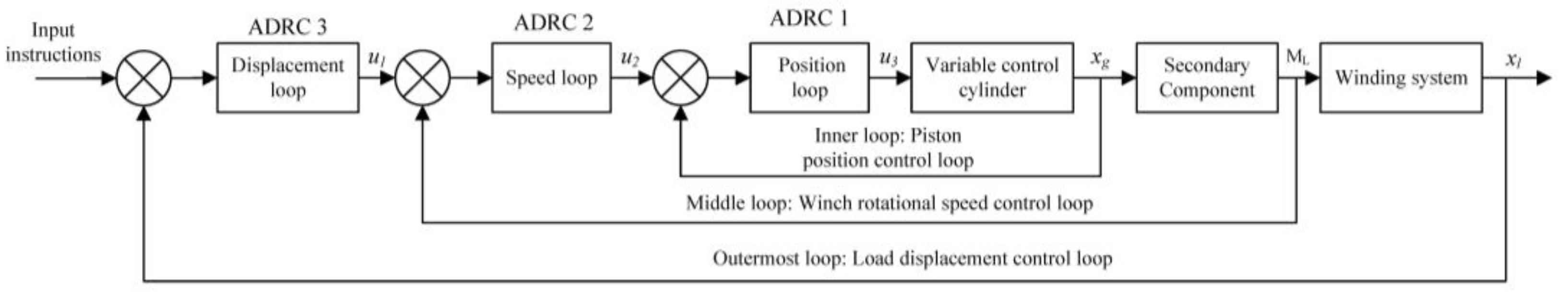
3. Three-Closed-Loop ADRC Position Control Strategy Design

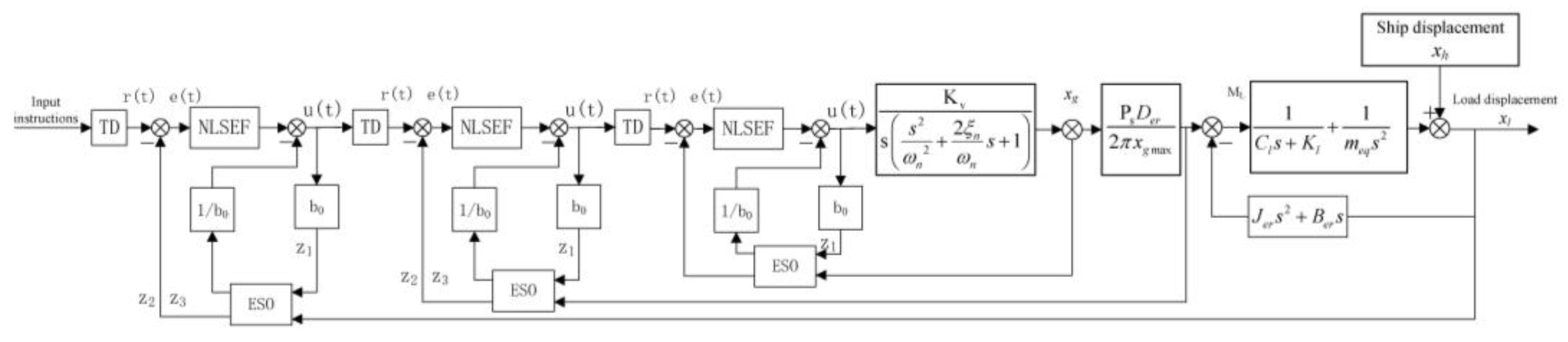
3.1. ADRC Controller Design and Composition

The active disturbance rejection control (ADRC) was invented by Jingqing Han to improve the PID controller [29]. Its basic principle is to extract real-time disturbance information from input and output signals and compensate for it through control force to achieve effective control. It has excellent disturbance rejection capabilities. The ADRC structure is shown in Figure 3 below.
Taking the heave compensation system as the controlled object, its algorithm mainly consists of four parts: the tracking differentiator, extended state observer, nonlinear state error feedback law, and disturbance estimation compensation.

3.1.1. The Tracking Differentiator (TD)

According to the reference signal r(t) and the given transition process r1(t), its derivative signal r2(t) can be computed. In the discrete form, it can be expressed as follows:
f h = f h a n r 1 k   r k , r 2 k , r , h 0 r 1 k + 1 = r 1 k + h r 2 k r 2 k + 1 = r 2 k + h · f h
where r is the velocity factor, and a larger value approaches the speed faster; h0 is the filtering factor; and h is the integration step size, where typically h0 can be equal to h, but to reduce overshoot and oscillations, h0 is usually taken to be greater than h.
fhan is the maximum speed control function, which has the following form:
d = r h 2 a 0 = h x 2 y = x 1 + a 0 a 1 = d d + 8 y a 2 = a 0 + s i g n ( y ) · ( a 1   d ) / 2 a = ( a 0 + y ) · f s g ( y , d ) + a 2 ( 1 f s g ( y , d ) ) f h a n = r ( a / d ) · f s g ( a , d ) r s i g n ( a ) · ( 1 f s g ( a , d ) )
The expression for the fsg function is
fsg x , d = sign x   + d sign x     d 2

3.1.2. Extended State Observer (ESO)

The extended state observer (ESO) is used to observe the state and disturbance of the controlled object. Its specific expression is as follows:
e = z 1     y fe = fal ( e , 0.5 , δ ) fe 1 = fal ( e , 0.25 , δ ) z 1 ˙ = z 1 + h ( z 2     β 01 e ) z 2 ˙ = z 2 + h ( z 3     β 02 fe + b 0 u ) z 3 ˙ = z 3 + h ( β 03 fe 1 )
The expression for the nonlinear function fal(e,α,δ) is as follows:
s = sign e + δ   sign e δ 2
fal e , α , δ = e   δ 1     α s   +   e α sign e 1     s
The parameters β01, β02, and β03 are observer gain parameters. The setting of these parameters can be determined based on the bandwidth method given by Gao Zhiqiang [30] as follows:
β 01 = 3 ω ,   β 02 = 3 ω 2 ,   β 03 = ω 3
where ω is the observer bandwidth. z1 is the estimated state signal, z2 is the estimated state velocity signal, and z3 is the estimated state acceleration signal.

3.1.3. Nonlinear States Error Feedback (NLSEF)

The system’s state error is determined by the difference between the outputs of ESO and TD. Then, the control law is determined based on the state error, as shown below:
u 0 = fhan e 1 , c e 1 e 2 , r , h 1
The equation includes u0, which represents the error feedback control signal.

3.1.4. Disturbance Estimation Compensation

The feedback control signal for the state error is compensated using the disturbance estimation value to determine the final control input to the controlled object. The form is as follows:
u = u 0 z 3 b 0
In this equation, b0 is the compensation factor. Increasing b0 can reduce the oscillations, but it will simultaneously decrease the compensation for disturbances, affecting the disturbance suppression effectiveness.

3.1.5. Stability Analysis

The ADRC controller designed in this article mainly referred to the paper by Jingqing Han [29]. As ADRC does not rely on the system model, the selection of controller parameters is based on the paper by Zhiqiang Gao [30]. The convergence of the observer and the stability of the ADRC controller are provided in more detail in Baozhu Guo’s published paper [31,32,33].

3.2. Controller Design and Parameter Setting

The design of the ADRC controller follows the principle of “inner loop before outer loop” to design a three-closed-loop position controller. The inner loop is the control loop for the piston displacement of the variable control cylinder, the middle loop is for the winch rotational speed control, and the outermost loop is for the load-displacement control. The parameter tuning begins with the inner control loop. By directly comparing the input signal and the output feedback signal of the inner loop, parameter tuning of a single-loop ADRC controller is achieved. Then, the parameter tuning continues with the next loop, namely, the rotational speed control loop. Since the inner loop has completed parameter tuning, it acts as a gain structure with a value of “1” in the control system, and its influence on the next loop can be neglected. Following the same method, parameter tuning is sequentially completed for the middle rotational speed loop and the outermost displacement loop.
Based on this, three second-order ADRC controllers are separately designed to construct the piston displacement loop, winch rotation speed loop, and load-displacement loop, forming the three-closed-loop ADRC. The control structure is illustrated in Figure 4.
Each controller structure is roughly the same. The input signal is denoted as r(t). It first undergoes processing through a tracking differentiator (TD) to obtain the differential signal and smooth command signals r1(t) and r2(t). The second-order extended state observer (ESO), which is established for each system, observes the feedback signals. Z1 represents the estimated state signal, Z2 is the estimated state velocity signal, and Z3 is the estimated state acceleration signal. The observer gain parameters β01, β02, and β03 are adjusted through the gain-scheduling method, and the tuning of these parameters can be determined using the bandwidth method provided by Gao Zhiqiang [30]. The specific control parameters are listed in Table 3. Finally, the signals r1(t) and r2(t) from the tracking differentiator (TD) and the signals Z from the extended state observer (ESO) are input into the nonlinear state error feedback (NLSEF) controller. By adjusting the compensation factor b0, the error and disturbance are estimated and compensated for.
The internal structure of the ADRC controller and the simulation model for the three-closed-loop ADRC position control are shown in Figure 5 and Figure 6, respectively. Using the bandwidth method, the parameters of each ADRC controller loop are tuned to achieve good control performance for load displacement.

4. Simulation Experiment Research and Analysis

In order to verify the superiority of the proposed controller over the PID controller in terms of compensation performance, we conducted simulation experiments in three disturbance environments while keeping the controller parameters unchanged: step disturbance, sine disturbance, and the measured heave disturbance of a mother ship in a certain sea area of China. The simulation results were compared and are discussed herein. In the simulation, the input load ideal position command was 0, and the winch was controlled to raise or lower the load for compensation response, thereby controlling the load to maintain the unchanged target position.
In order to facilitate better result comparisons, the compensation rate ζ and load position error Δ were defined to represent the efficiency and accuracy of the compensation strategy.
The root-mean-square difference compensation rate ζ in the heave compensation was defined as
ζ = 1 1 T 0 T x x ^ 2 x 2
The load position error Δ in heave compensation:
Δ = | x x ^ |
The maximum position error Δmax in heave compensation:
Δ max   = max 0 t T | x x ^ |
In these equations, T is the statistical duration, x is the amplitude of the disturbance at time t, and x^ is the amplitude of the system response at time t.

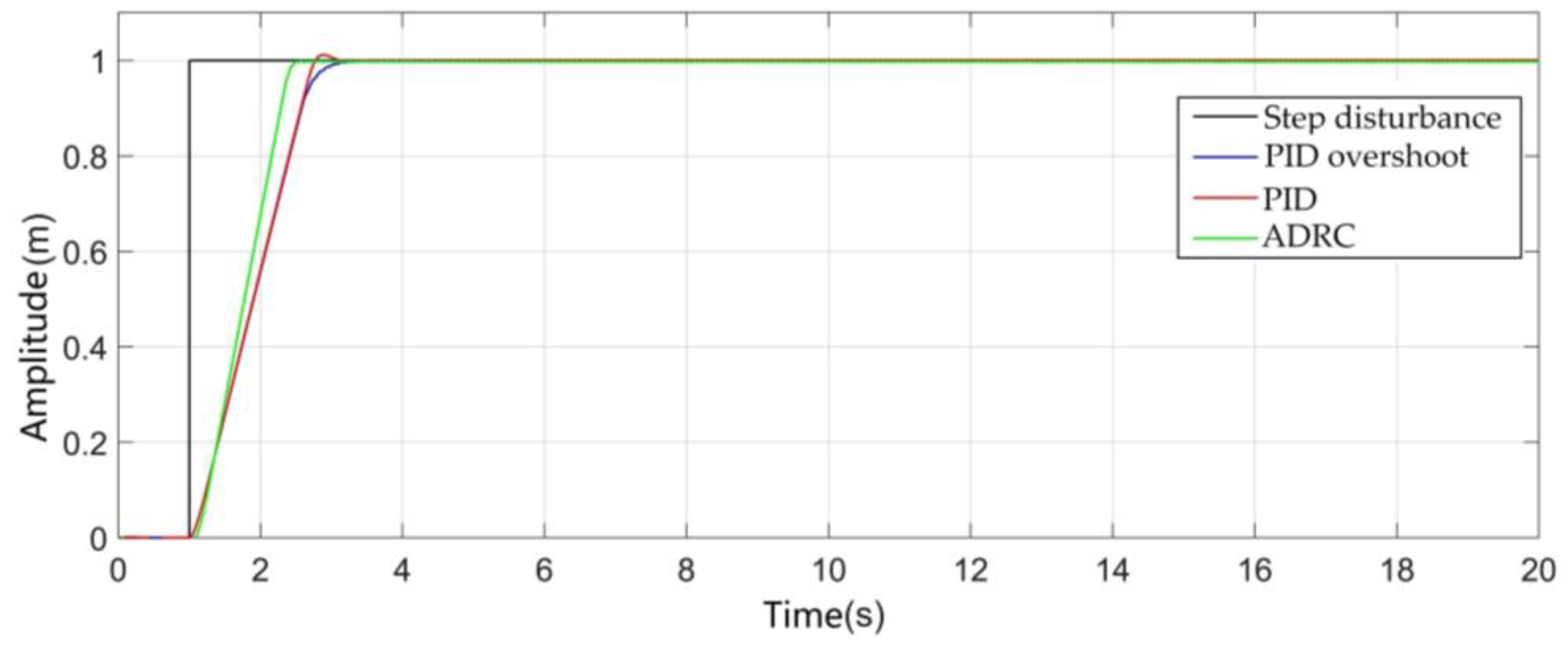
4.1. Step Disturbance Response Analysis

To compare the dynamic performance of the three-closed-loop PID control system and the three-closed-loop ADRC system, a step disturbance signal was applied to the designed simulation system model. As shown in Figure 7, the given step signal had an amplitude of 1 m, starting from 1 s.
The simulation results were input into MATLAB, then the stepinfo function was used to extract the step response metrics for each curve, as shown in Table 4.
The parameters of the PID controller consisted of two sets: one set for the no-overshoot condition and another set that with a slight adjustment, introduced a small overshoot. By comparing the step response curves of the two PID sets with the step response curve of the ADRC, it was evident that the three-closed-loop ADRC system had a faster response speed. Even when adjusting the PID parameters to induce overshoot, the system’s response did not significantly accelerate. This indicates that the classical PID controller indeed faced a trade-off between speed and overshoot. The rise time of the ADRC was about 0.3 s faster than the PID. In contrast, the three-closed-loop ADRC controller designed in this study effectively addressed this trade-off.

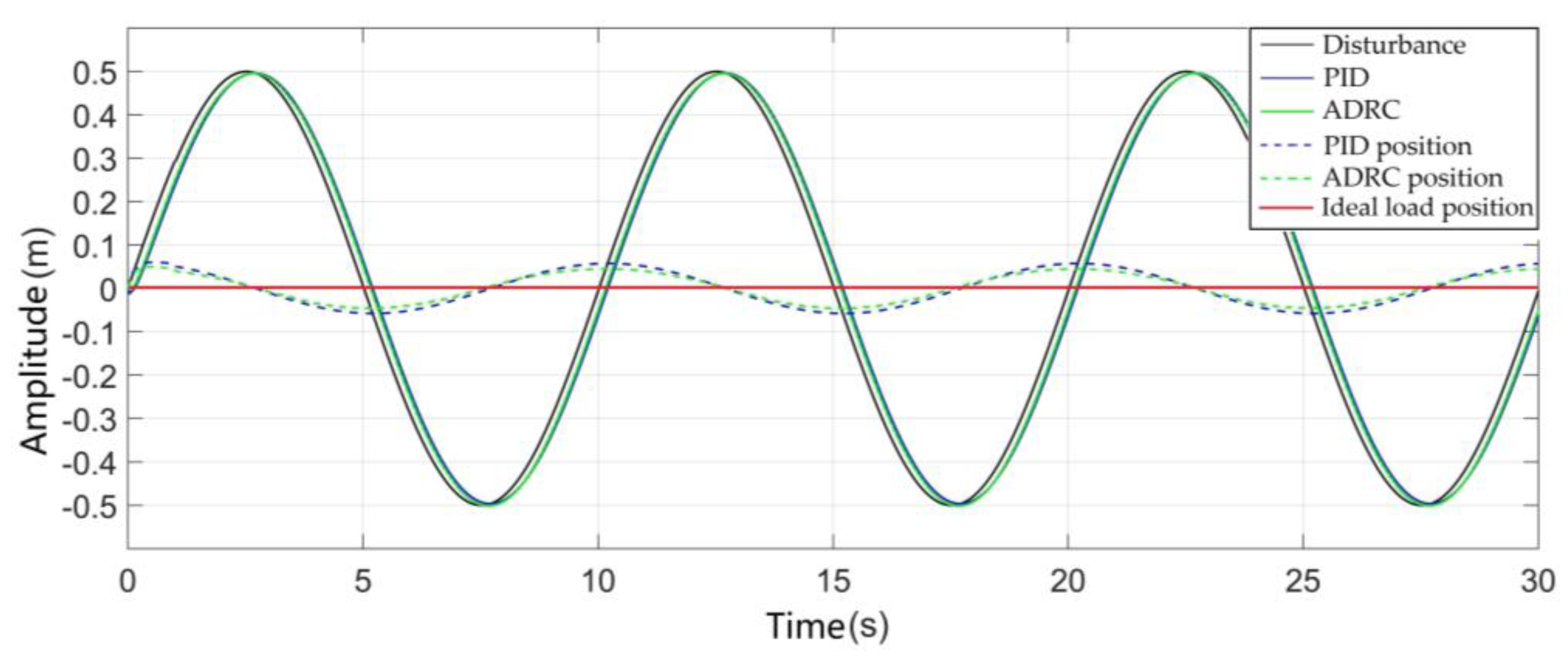
4.2. Sine Disturbance Response Analysis

Taking a condition close to sea state 3, a sine disturbance curve with an amplitude of 0.5 m and a period of 10 s was selected for the simulation, as shown in Figure 8.
The black curve represents the input disturbance signal, namely, the given sinusoidal command signal. The solid blue line depicts the system response under three-closed-loop PID control, while the solid green line represents the system response under three-closed-loop ADRC. The dashed blue line illustrates the load position curve after compensation in the three-closed-loop PID control system, and the dashed green line denotes the load position curve after compensation in the three-closed-loop ADRC system. We expected the load position to remain stable at amplitude 0 and remain stationary. The solid red line represents the ideal load position. From the graph, it can be observed that during the startup phase, the three-closed-loop ADRC system exhibited better dynamic performance compared with the three-closed-loop PID control system. It quickly responded to the input sine disturbance signal, and during the subsequent tracking motion, the phase lag between the tracking curve of the three-closed-loop ADRC system and the input disturbance signal was smaller compared with the three-closed-loop PID control system. This consequently led to the efficiency and precision of the compensation system, namely, the compensation rate ζ and load position error Δ in the heave compensation.
Based on the simulation results, when a sine disturbance curve with an amplitude of 0.5 m and a period of 10 s was input into the systems, ignoring the initial startup phase, the load position max error Δmax for the three-closed-loop PID control system was 0.061 m, and for the three-closed-loop ADRC system, it was 0.045 m. The compensation rate ζ values for the three-closed-loop PID control system and the three-closed-loop ADRC system were 83.46% and 91.52%, respectively. The designed three-closed-loop ADRC controller exhibited better compensation performance under the sine disturbance.

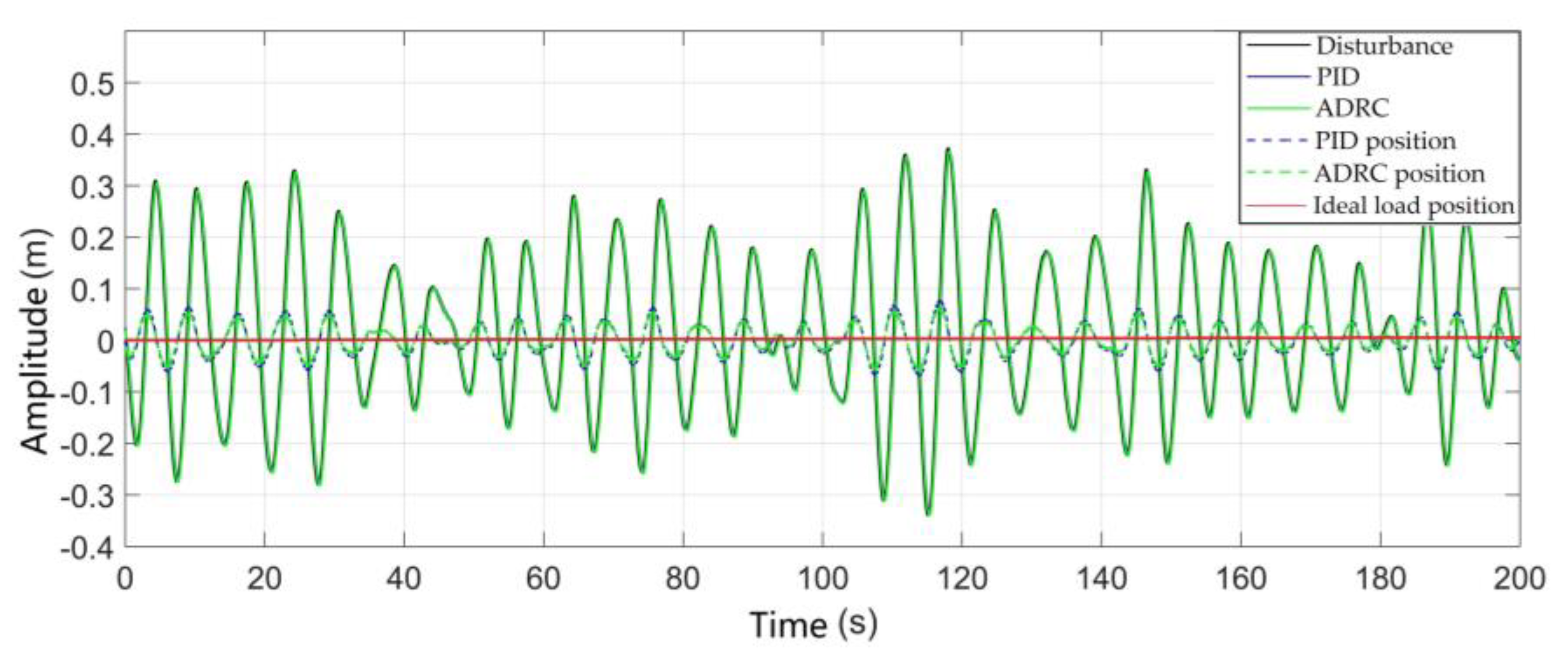
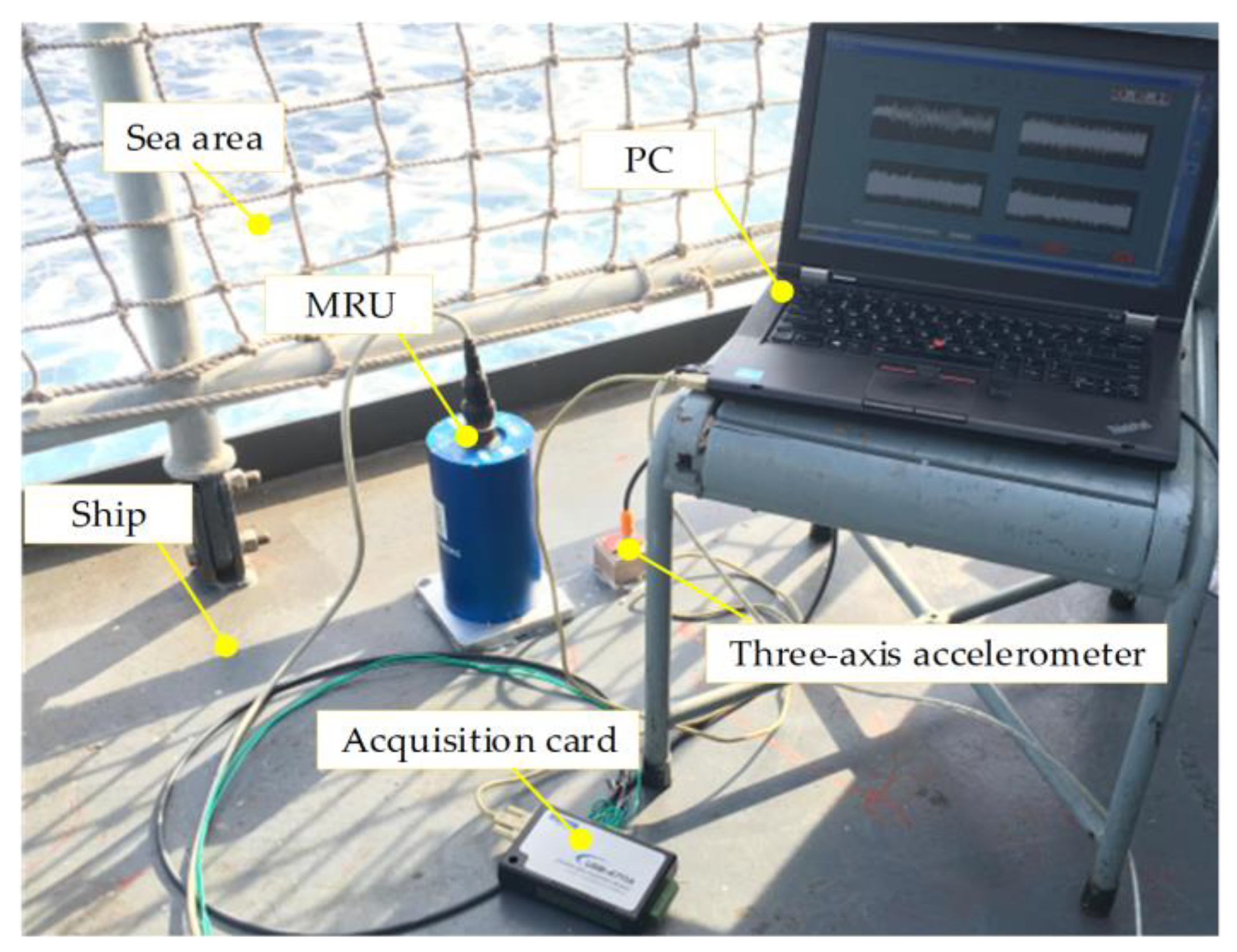
4.3. A Certain Sea Area in China Ship Heave Motion Disturbance Response Analysis

The heave disturbance response of a measured ship in a certain sea area in China simulated the heave disturbance experienced by the actual load in real sea waves. The actual heave motion data of the ship in a certain sea area in China were collected using a motion reference unit (MRU), as shown in Figure 9. The measured heave motion of the ship served as the disturbance input in the simulation experiments. To enhance the performance of the compensation controller, the measured disturbance input needed to undergo data processing and filtering, as shown in Figure 10.
The simulation of the heave motion curve responses for a certain sea area in China was conducted for the three-closed-loop ADRC position control system and the no-overshoot three-closed-loop PID position control system. The results are shown in Figure 11 and Figure 12.
According to the simulation results, the maximum amplitude of the measured heave motion for the ship was 0.374 m. Under the compensation of the three-closed-loop PID control system, the maximum load position error Δmax was ±0.079 m and the compensation rate ζ was 75.16%. Under the compensation of the three-closed-loop ADRC system, the maximum load position error Δmax was ±0.061 m and the compensation rate ζ was 90.81%. The compensation rate increased by 15.65%. Therefore, whether in step disturbance, sine disturbance, or disturbance according to the measured heave motion of the ship, the designed three-closed-loop ADRC position control system exhibited faster dynamic characteristics, a better compensation rate, and a smaller load position error.
Figure 13 shows a local magnification of the simulation curve of the measured heave motion for the ship under the three-closed-loop control system. From the figure, it can be observed that there was a phase delay of less than 0.2 s in the system. This was due to the large inertia of the winch compensation system, resulting in a response delay in the system, and the presence of delay in the ship heave motion sensor, causing a phase delay, thereby affecting the accuracy of position compensation. This issue can be improved by predicting the heave motion of the ship.

5. Conclusions

For a winch-based active heave compensation system, a three-closed-loop ADRC position compensation strategy based on a winch-type heave compensation system with a secondary component is proposed. The ADRC controllers for each loop compensate for the total disturbance information extracted in real time from the input and output signals, achieving better control performance and excellent disturbance rejection capability. By tuning the parameters of each ADRC loop, a superior control effect on load displacement is ultimately achieved, enhancing the compensation performance.
The proposed three-closed-loop ADRC position compensation strategy based on a winch-type heave compensation system with a secondary component achieves accurate and rapid position tracking control under various sea conditions. Under the condition of the maximum amplitude of 0.374 m in the measured heave motion of the ship in a certain sea area in China, the winch-based heave compensation system with the secondary component using the three-closed-loop ADRC position control achieved a maximum load position error of ±0.061 m, with a compensation rate of 90.81%, demonstrating excellent heave compensation performance.
In the control of the load position, the time delay effects caused by system inertia, sensor accuracy, and data filtering have a significant impact on heave compensation. In future work, improving the performance of the heave compensation system can be achieved by incorporating ship motion prediction or employing more advanced controllers.

Author Contributions

Conceptualization, S.L., Y.L. and F.Y.; methodology, Q.W. and F.Y.; software, Q.W. and L.Q.; validation, Q.W., Y.L. and Z.G.; formal analysis, L.Q. and Y.L.; investigation, Y.L. and F.Y; resources, S.L. and Y.L.; data curation, L.Q. and Z.G.; writing—original draft preparation, Q.W. and F.Y.; writing—review and editing, S.L., Q.W. and F.Y.; visualization, Z.G.; project administration, S.L. and F.Y. All authors have read and agreed to the published version of the manuscript.

Funding

This research was funded by the National Natural Science Foundation of China (General Program, grant number 2021SDDR228) and Excellent Youth Foundation of Shandong Scientific Committee (grant number B8D9B198A48D6A25E053BE07C2CAC8E8).

Institutional Review Board Statement

Not applicable.

Informed Consent Statement

Not applicable.

Data Availability Statement

Data are contained within the article.

Conflicts of Interest

Author Yufeng Liu was employed by the company Taiyuan Heavy Machinery Group Yuci Hydraulic Industry (Jinan) Co., Ltd., Author Longfei Qiao was employed by the company Cnooc Energy Logistics Co., Ltd., The remaining authors declare that the research was conducted in the absence of any commercial or financial relationships that could be construed as a potential conflict of interest.

Appendix A

Table A1. Abbreviation definitions.
AcronymsDefinition
ADRCActive disturbance rejection control
PIDProportional integral derivative
AMESimSoftware name
A4VSO, A4VSGRexroth product model
HNCRexroth controller
AHCActive heave compensation system
SMCSliding mode control
MPCModel predictive control
IDA-PBCInterconnection and damping assignment
productivity based control
ABFTSMCAdaptive barrier fast terminal sliding mode control
UAVsUnmanned aerial vehicles
FTSMCFast terminal sliding mode control
NMPCNonlinear model predictive control
TDTracking differentiator
ESOExtended state observer
NLSEFNonlinear states error feedback
MRUMotion reference unit
Table A2. Variable explanation table.
SymbolDefinitionSymbolDefinition
QsfOutput flowθerMain shaft rotation angle of the secondary component
ICoil input currentBerViscous damping coefficient
KvFlow gainMLExternal load torque
sLaplace operatorxlDisplacement of the load
ωnNatural frequencyxl0Initial position of the load
ξnDamping ratioxhDisplacement due to the heave of the ship
qFlow entering the high-pressure chamberijtReduction ratio of the gearbox
AgEffective piston area insideRRadius of the winch drum
xgPiston displacementΔlElongation of the cable
CtTotal leakage coefficientΔldDynamic elongation of the cable
pPressure differenceΔlsStatic elongation of the cable
VtTotal volumemeqEquivalent mass of the load and cable
βeVolumetric modulus of oilklCable’s elastic coefficient
CiInternal leakage coefficientClCable’s damping coefficient
CeExternal leakage coefficientrVelocity factor
mgTotal mass of the moving componentsh0Filtering factor
BgViscous damping coefficienthIntegration step size
kgSpring stiffnessfhanMaximum speed control function
FfgResistance force actingβ01, β02, β03Observer gain parameters
DerSecondary component displacementb0Compensation factor
DermaxSecondary component maximum displacementζHeave compensation root-mean-square error compensation rate
xgmaxMaximum displacement of the pistonΔLoad position error in heave compensation
psConstant pressure of the oil supplyTStatistical duration
JerRotational inertia converted to the output shaftxAmplitude of the disturbance

References

  1. Woodacre, J.K.; Bauer, R.J.; Irani, R.A. A Review of Vertical Motion Heave Compensation Systems. Ocean Eng. 2015, 104, 140–154. [Google Scholar] [CrossRef]
  2. Petillot, Y.R.; Antonelli, G.; Casalino, G.; Ferreira, F. Underwater Robots: From Remotely Operated Vehicles to Intervention-Autonomous Underwater Vehicles. IEEE Robot. Autom. Mag. 2019, 26, 94–101. [Google Scholar] [CrossRef]
  3. Yu, H.; Chen, Y.; Shi, W.; Xiong, Y.; Wei, J. State Constrained Variable Structure Control for Active Heave Compensators. IEEE Access 2019, 7, 54770–54779. [Google Scholar] [CrossRef]
  4. Woo, N.-S.; Kim, H.-J.; Han, S.-M.; Ha, J.-H.; Huh, S.-C.; Kim, Y.-J. Evaluation of the Structural Stability of a Heave Compensator for an Offshore Plant and the Optimization of Its Shape. J. Nanosci. Nanotechnol. 2020, 20, 263–269. [Google Scholar] [CrossRef] [PubMed]
  5. Xie, T.; Zou, D.; Huang, L.; Liu, D. Modelling and Simulation Analysis of Active Heave Compensation Control System for Marine Winch. In Proceedings of the 2021 IEEE 4th International Electrical and Energy Conference (CIEEC), Wuhan, China, 28 May 2021; pp. 1–6. [Google Scholar] [CrossRef]
  6. Jakubowski, A.; Milecki, A. The Investigations of Hydraulic Heave Compensation System. In Automation 2018; Szewczyk, R., Zieliński, C., Kaliczyńska, M., Eds.; Advances in Intelligent Systems and Computing; Springer International Publishing: Cham, Switzerland, 2018; Volume 743, pp. 380–391. ISBN 978-3-319-77178-6. [Google Scholar] [CrossRef]
  7. Dabing, Z.; Jianzhong, W.; Xin, L. Ship-Mounted Crane’s Heave Compensation System Based on Hydrostatic Secondary Control. In Proceedings of the 2011 International Conference on Mechatronic Science, Electric Engineering and Computer (MEC), Jilin, China, 19–22 August 2011; pp. 1626–1628. [Google Scholar] [CrossRef]
  8. Busquets, E.; Ivantysynova, M. Adaptive Robust Motion Control of an Excavator Hydraulic Hybrid Swing Drive. SAE Int. J. Commer. Veh. 2015, 8, 568–582. [Google Scholar] [CrossRef]
  9. Liu, T.; Iturrino, G.; Goldberg, D.; Meissner, E.; Swain, K.; Furman, C.; Fitzgerald, P.; Frisbee, N.; Chlimoun, J.; Van Hyfte, J.; et al. Performance Evaluation of Active Wireline Heave Compensation Systems in Marine Well Logging Environments. Geo-Mar. Lett. 2013, 33, 83–93. [Google Scholar] [CrossRef]
  10. Moslått, G.-A.; Rygaard Hansen, M.; Padovani, D. Performance Improvement of a Hydraulic Active/Passive Heave Compensation Winch Using Semi Secondary Motor Control: Experimental and Numerical Verification. Energies 2020, 13, 2671. [Google Scholar] [CrossRef]
  11. Zinage, S.; Somayajula, A. Deep Reinforcement Learning Based Controller for Active Heave Compensation. IFAC-PapersOnLine 2021, 54, 161–167. [Google Scholar] [CrossRef]
  12. Sun, Y.G.; Qiang, H.Y.; Sheng, X.M. Genetic Algorithm-Based Parameters Optimization for the PID Controller Applied in Heave Compensation System. Appl. Mech. Mater. 2014, 556–562, 2462–2465. [Google Scholar] [CrossRef]
  13. Feng, Y.; Yu, X.; Han, F. On Nonsingular Terminal Sliding-Mode Control of Nonlinear Systems. Automatica 2013, 49, 1715–1722. [Google Scholar] [CrossRef]
  14. Mayne, D.Q. Model Predictive Control: Recent Developments and Future Promise. Automatica 2014, 50, 2967–2986. [Google Scholar] [CrossRef]
  15. Tianxiang, M.; Yi, Y.; Jianbo, C.; Guihong, Z.; Yuanpei, Y.; Jianshan, W.; Haiqin, G.; Hui, Y. Design of Heave Compensation Control System Based on Variable Parameter PID Algorithm. In Proceedings of the 2018 Chinese Control and Decision Conference (CCDC), Shenyang, China, 9–11 June 2018; pp. 825–829. [Google Scholar] [CrossRef]
  16. Do, K.D.; Pan, J. Nonlinear Control of an Active Heave Compensation System. Ocean Eng. 2008, 35, 558–571. [Google Scholar] [CrossRef]
  17. Kuchler, S.; Sawodny, O. Nonlinear Control of an Active Heave Compensation System with Time-Delay. In Proceedings of the 2010 IEEE International Conference on Control Applications, Yokohama, Japan, 8–10 September 2010; pp. 1313–1318. [Google Scholar] [CrossRef]
  18. Zhou, H.; Cao, J.; Yao, B.; Lian, L. Hierarchical NMPC–ISMC of Active Heave Motion Compensation System for TMS–ROV Recovery. Ocean Eng. 2021, 239, 109834. [Google Scholar] [CrossRef]
  19. Zhang, Q.; Tan, B.; Hu, X. Ship Heave Compensation Based on PID-DDPG Hybrid Control. In Proceedings of the 2023 42nd Chinese Control Conference (CCC), Tianjin, China, 24 July 2023; pp. 8576–8581. [Google Scholar]
  20. Guerrero-Sanchez, M.-E.; Hernandez-Gonzalez, O.; Valencia-Palomo, G.; Lopez-Estrada, F.-R.; Rodriguez-Mata, A.-E.; Garrido, J. Filtered Observer-Based IDA-PBC Control for Trajectory Tracking of a Quadrotor. IEEE Access 2021, 9, 114821–114835. [Google Scholar] [CrossRef]
  21. Najafi, A.; Vu, M.T.; Mobayen, S.; Asad, J.H.; Fekih, A. Adaptive Barrier Fast Terminal Sliding Mode Actuator Fault Tolerant Control Approach for Quadrotor UAVs. Mathematics 2022, 10, 3009. [Google Scholar] [CrossRef]
  22. Zhou, R.; Neusypin, K.A. ADRC-Based UAV Control Scheme for Automatic Carrier Landing. In Proceedings of the 15th International Conference “Intelligent Systems” (INTELS’22), Moscow, Russia, 14–16 December 2022; p. 66. [Google Scholar] [CrossRef]
  23. Deng, B.; Xu, J. Trajectory Tracking Based on Active Disturbance Rejection Control for Compound Unmanned Aircraft. Aerospace 2022, 9, 313. [Google Scholar] [CrossRef]
  24. Li, Z.; Ma, X.; Li, Y.; Meng, Q.; Li, J. ADRC-ESMPC Active Heave Compensation Control Strategy for Offshore Cranes. Ships Offshore Struct. 2020, 15, 1098–1106. [Google Scholar] [CrossRef]
  25. Shuguang, L.; Wuyang, C.; Kecheng, W.; Jia, J. An ADRC-Based Active Heave Compensation for Offshore Rig. In Proceedings of the 2020 Chinese Control and Decision Conference (CCDC), Hefei, China, 22–24 August 2020; pp. 2979–2984. [Google Scholar] [CrossRef]
  26. Messineo, S.; Serrani, A. Offshore Crane Control Based on Adaptive External Models. Automatica 2009, 45, 2546–2556. [Google Scholar] [CrossRef]
  27. Li, M.; Gao, P.; Zhang, J.; Gu, J.; Zhang, Y. Study on the System Design and Control Method of a Semi-Active Heave Compensation System. Ships Offshore Struct. 2018, 13, 43–55. [Google Scholar] [CrossRef]
  28. Röper, R. ölhydraulik und Pneumatik. In Dubbel; Beitz, W., Küttner, K.-H., Eds.; Springer: Berlin/Heidelberg, Germany, 1987; pp. 597–616. ISBN 978-3-662-06779-6. [Google Scholar] [CrossRef]
  29. Han, J. From PID to Active Disturbance Rejection Control. IEEE Trans. Ind. Electron. 2009, 56, 900–906. [Google Scholar] [CrossRef]
  30. Gao, Z.; Huang, Y.; Han, J. An Alternative Paradigm for Control System Design. In Proceedings of the 40th IEEE Conference on Decision and Control (Cat. No.01CH37228), Orlando, FL, USA, 4–7 December 2001; Volume 5, pp. 4578–4585. [Google Scholar] [CrossRef]
  31. Guo, B.-Z.; Zhao, Z. On the Convergence of an Extended State Observer for Nonlinear Systems with Uncertainty. Syst. Control Lett. 2011, 60, 420–430. [Google Scholar] [CrossRef]
  32. Guo, B.-Z.; Zhao, Z.-L. On Convergence of the Nonlinear Active Disturbance Rejection Control for MIMO Systems. SIAM J. Control Optim. 2013, 51, 1727–1757. [Google Scholar] [CrossRef]
  33. Guo, B.-Z.; Wu, Z.-H. Output Tracking for a Class of Nonlinear Systems with Mismatched Uncertainties by Active Disturbance Rejection Control. Syst. Control Lett. 2017, 100, 21–31. [Google Scholar] [CrossRef]
Figure 1. Winch heave compensation system based on a secondary component.
Jmse 12 00346 g001
Figure 2. Structure diagram of heave compensation control.
Jmse 12 00346 g002
Figure 3. ADRC algorithm block diagram.
Jmse 12 00346 g003
Figure 4. Three closed-loop ADRC block diagram.
Jmse 12 00346 g004
Figure 5. The internal structure of the ADRC controller.
Jmse 12 00346 g005
Figure 6. Three-closed-loop ADRC position control simulation model.
Jmse 12 00346 g006
Figure 7. Simulation curve of step disturbance response of three-closed-loop control system.
Jmse 12 00346 g007
Figure 8. The sine disturbance response curve of three-closed-loop position control system with amplitude 0.5 m and period 10 s.
Jmse 12 00346 g008
Figure 9. Photographs of MRU measurement of ship heave motion data.
Jmse 12 00346 g009
Figure 10. Comparison of measured curves was processed by filtering.
Jmse 12 00346 g010
Figure 11. Simulation curve of measured ship heave curve of three-closed-loop control system.
Jmse 12 00346 g011
Figure 12. Load position curve of measured ship heave curve of three-closed-loop control system.
Jmse 12 00346 g012
Figure 13. Local magnification of the simulation curve for the heave motion of the ship under the three-closed-loop control system.
Jmse 12 00346 g013
Table 1. Sub-models of the main components in the hydraulic system simulation model.
Main ComponentsSub-ModelFunctional Description
MotorPM000Standard electric motor
PumpPP01Constant-pressure variable pump
Servo valveSV00Three-position four-way
directional valve
Relief valveRV012Safety valve
AccumulatorHA000Diaphragm-type accumulator
Variable cylinder spring chamberBAP016Variable cylinder reset
function chamber
Variable cylinder piston chamberBAF01Variable cylinder control
function chamber
Mass blockMECMAS21/MAS001Variable cylinder mass
property simulation
Hydraulic motorHYDVPM01Bidirectional variable hydraulic motor
WinchWINCH01Ideal winch
Cable or wire ropeMECROPE0/REND001Rigid rope
Table 2. Main parameters of the simulation model.
Parameter NameValueUnit
Hydraulic motor displacement Der40mL/r
Maximum motor speed nmdmax664r/min
Gearbox reduction ratio ijt26.4
Winch drum radius R190mm
System pressure ps18MPa
Accumulator volume V20L
Table 3. Three-closed-loop ADRC controller parameters.
ParametershrTDrNLSEFβ01β02β03b0
Inner loop ADRC0.001 1 × 10 7 5 × 10 7 10000 1 × 10 7 1 × 10 8 / 3 1 × 10 6
Middle loop ADRC0.001900 1 × 10 5 10000 3.75 × 10 7 6 . 25 × 10 10 780
Outermost loop ADRC0.001900 4.5 × 10 5 10000 3.75 × 10 7 6 . 25 × 10 10 7500
Table 4. Step response index evaluation table.
ParametersRise Time (s)Peak Time (s)Maximum
Overshoot
Settling
Time (s)
No-overshoot PID1.34452.340001.7077
Overshoot PID1.33471.89001.18%1.6563
ADRC1.02571.570001.3532
Note: settling time is the time required for the response curve to reach and stay within a 5% error range of the steady-state value.
Disclaimer/Publisher’s Note: The statements, opinions and data contained in all publications are solely those of the individual author(s) and contributor(s) and not of MDPI and/or the editor(s). MDPI and/or the editor(s) disclaim responsibility for any injury to people or property resulting from any ideas, methods, instructions or products referred to in the content.

