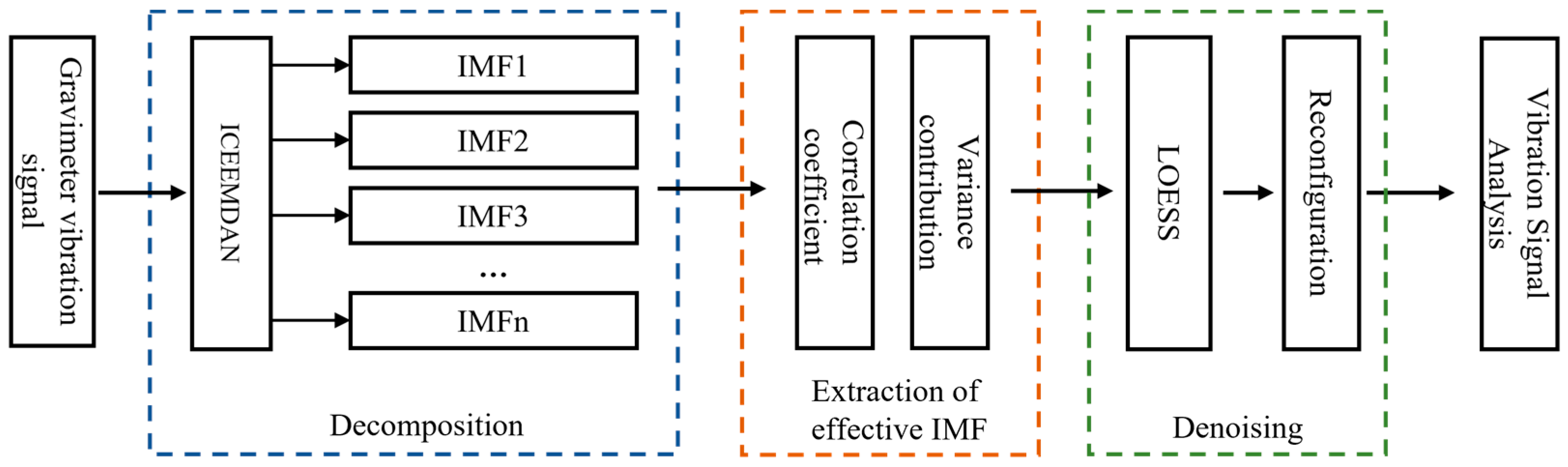
ICEEMDAN/LOESS: An Improved Vibration-Signal Analysis Method for Marine Atomic Interferometric Gravimetry

Abstract

The marine atomic interferometric gravimeter is a vital precision instrument for measuring marine geophysical information, which is widely used in mineral resources exploration, military applications, and missile launches. In practical measurements, vibration disturbance is an important factor that affects measurement accuracy. This paper proposes the combination of improved complete ensemble empirical mode decomposition with adaptive noise and locally weighted regression for vibration characterization of gravimeter vibration data. Firstly, the original signal is added into a pair of white noise for adaptive noise-complete ensemble empirical mode decomposition to obtain multiple intrinsic mode functions. The efficient IMF components and noise components are filtered out under the dual indicators of correlation coefficient and variance contribution ratio, and then the LOESS filtering method is used for noise reduction to obtain useful signal detail information; finally, the noise-containing components are reconstructed with the effective components after the noise-reduction process. The experimental results of both simulated and measured vibration signals show that the proposed method can effectively decompose the different high- and low-frequency bands contained in the vibration signal and remove the noise of the original signal.

1. Introduction

High-precision marine atomic interferometric gravimetry [1,2,3] can be used in mineral resources exploration, geological structure research, military science research, and other engineering and technical fields [4,5,6], which are characterized by continuous high-precision measurements for a long time, but a series of complex technical problems need to be solved to improve the experimental accuracy of measuring gravitational acceleration [7,8,9]. In actual measurements, the accuracy of atomic gravity measurements is often affected by various types of noise, like ground vibration noise. For example, the noise from human activities (generally greater than 1 Hz), the noise from the Earth’s internal motion (generally in the range of 0.1 to 30 Hz), and the noise from atmospheric movement (typically less than 0.1 Hz), contribute to this noise. These vibration disturbances accompany the measurement process, which is difficult for customer service but cannot be ignored. How to further improve the measurement accuracy and reduce the vibration-noise interference of cold atomic gravimeters [10] is an important research direction in this field.

The vibration signal of atomic interference gravimeter is a complex non-stationary time-varying signal, and the traditional time-domain or frequency-domain analysis methods make it difficult to extract the characteristic information of vibration accurately, and it is not easy to analyze the vibration characteristics. For example, the short-time Fourier transform [11] is suitable for the analysis of slowly changing signals and is a smooth signal analysis method; the wavelet transform [12] is widely used in rotational vibration-signal processing because of its multi-resolution characteristics, but the wavelet base selection in the wavelet transform has a great influence on the analysis results, and once a certain wavelet base is determined, it cannot be changed during the whole analysis process. Therefore, the wavelet transform lacks self-adaptability for signal processing. For such problems, the empirical mode decomposition (EMD) proposed by Huang [13] is very classical, which automatically decomposes the signal into a finite number of IMF components based on the signal characteristics, with good adaptive performance, and is particularly good in dealing with nonlinear and non-stationary signals. Once proposed, modal decomposition has received wide attention and has been successfully applied to several fields. Its versatility and effectiveness make it a valuable tool for researchers and engineers in diverse domains. Tang [14] used the morphological singular value decomposition filtering noise-reduction method to denoise the vibration signal, then used the EMD algorithm to extract the fault features in the signals, and the experimental results verified that the approach could effectively obtain the bearing fault feature information. Meanwhile, Zhan [15] derived an EMD-based time-frequency denoising algorithm to accomplish the extraction of the efficient components of the multi-frequency mixed signal, realized the self-sensing of the vibration signal of ultrasonic-assisted grinding equipment, and verified the noise-reduction performance of the proposed algorithm through numerical simulations and self-sensing experiments. Zhong [16] used an improved ensemble empirical mode decomposition (EEMD) and depth belief network (DBN) approach to extract bearing speed features and perform vibration analyses. The simulation results on rolling bearing data at the Case Western Reserve University Bearing Data Center showed the effectiveness of the proposed method. Zhou [17] used a neural network model using the EEMD algorithm to reduce the effect of the non-smoothness of short-time marine vessel traffic flow and combine it with an optimized long short-term memory (LSTM) for the prediction of short-time vessel traffic flow. Yang [18] used the combined method of complete ensemble empirical mode decomposition with adaptive noise (CEEMDAN) and wavelet packet adaptive thresholding for noise reduction in acoustic emission signals, which improved denoising performance remarkably and effectively retained the characteristic information of acoustic emission signals. However, the EMD method has different degrees of endpoint effects and modal aliasing problems in the application process, which brings some issues to the signal decomposition.

Therefore, this paper proposes an improved method combining adaptive noise-complete ensemble empirical mode decomposition (ICEEMDAN) and locally weighted regression filtering (LOESS) to study and analyze the vibration signals of the oceanic atomic interferometric gravimeter. The analog signal and the measured vibration data of the gravimeter are decomposed to reduce the noise, and the frequency band composition of the vibration signal is analyzed to provide theoretical support for the design of the vibration isolation system of the gravimeter. This paper is organized as follows: Section 2 introduces the ICEEMDAN method. Section 3 uses simulation signals to explain the details of the proposed ICEEMDAN and LOESS filtering. Section 4 applies this method to the vibration-signal analysis of atomic gravimeters. Section 5 concludes this paper.

2. Materials and Methods

After obtaining the original vibration signal of the ocean atomic gravimeter, we propose a combined method based on improved complete ensemble empirical mode decomposition with adaptive noise and locally weighted regression filtering to process the original signal according to the idea of decomposition–extraction effective IMF-filter reconstruction; the processing flow is shown in Figure 1.

2.1. Improved Complete Ensemble EMD

The series of empirical mode decomposition methods decompose non-stationary signals that may come from nonlinear systems in a local and complete data-driven manner, but their decomposed signals suffer from the problem of modal aliasing, and there is always some residual white noise in the obtained eigenmodal components, which affects the subsequent analysis and processing of the signals. The improved complete ensemble empirical mode decomposition with adaptive noise aims to solve the components’ residual noise and pseudo morality problem.

The algorithm introduces two operators: (1) the operator $E_k(·)$, which produces the kth IMF obtained by EMD, and (2) the operator $M(·)$, which produces the local mean of the signal that is applied. The local mean refers to the “original signal minus this IMF component”. Then, the following steps are applied:

Step 1:

Define $x$ as the signal to be decomposed and $\beta$ as a constant coefficient. Let $w^{(i)}$ be a realization of white Gaussian noise with zero and unit variance.

Step 2:

Add group I white noise $w^{(i)}$ to the original signal, construct the sequence $x^{(i)}=x+{\beta }_{0}E(w^{(i)})$, and obtain the first set of residuals $R_1=(M(x^{(i)}))$.

Step 3:

Calculate the first modal component $d_1=x-R_1$.

Step 4:

Continue adding white noise, calculate the second set of residuals $R_1+{\beta }_{1}E(w^{(i)})$ using local mean decomposition, and define the second modal component $d_2$, $d_2=R_1-R_2=R_1-(M(R_1+{\beta }_{1}E(w^{(i)})))$.

Step 5:

Calculate the Kth residual $M(R_{k-1}+{\beta }_{k-1}E(w^{(i)}))$ and the modal component $d_k=R_{k-1}-R_k$.

Step 6:

Until the end of the computational decomposition, all modalities and residual numbers are obtained.

2.2. Determination of the Effective IMF Component

The principle of ICEEMDAN shows that the original signal can acquire a set of IMF components with different characteristic scales after decomposition, and these IMF components show different vibration characteristics of the signal. Due to the complexity of the signal acquisition environment and the influence of noise and other conditions, the decomposed signal contains noise components and spurious components, and all these factors are not conducive to the subsequent characterization of the signal, so it is necessary to filter the IMF components and select the IMF components with better correlation with the original signal, which better reflects the information contained in the original signal.

We determine the number of IMF components using the correlation coefficient Cor and variance contribution rate [19,20,21] VarR in this paper, which are calculated as shown in Equations (1) and (2). The larger the Cor, the better the correlation between the IMF component and the original signal, which better reflects the physical information of the original signal. On the contrary, a smaller Cor indicates that the correlation between the IMF component and the original signal is poor, which is not conducive to the analysis of the original signal and can be regarded as redundant information. The same is true for the variance contribution rate.

$$Cor=\frac{{\displaystyle \sum _{i=1}^N\left(x(i)-\overline{x}\right)\left(c_j(i)-\overline{c_j}\right)}}{{\left[{\displaystyle \sum _{i=1}^N{\left(x(i)-\overline{x}\right)}^2{\displaystyle \sum _{i=1}^N{\left(c_j(i)-\overline{c_j}\right)}^2}}\right]}^{1/2}}$$

(1)

$$VarR=\frac{{\displaystyle \sum _{i=1}^N{\left(c(i)-\overline{c}\right)}^2}}{{\displaystyle \sum _{i=1}^N{\left(x(i)-\overline{x}\right)}^2}}$$

(2)

where N denotes the length of the signal, $x(i)$ refers to the original signal, $c(i)$ represents the IMF component.

2.3. Noise Signal Filtering

In this work, the locally weighted regression filtering method (LOESS) [22] will be used to filter the noisy signal. This filtering method can decompose the observed data into a smooth part and a perturbed part. In the calculation process, the LOESS filtering method requires half-span parameters in both the x and y directions to determine the size of the filter window, which is the number of data points included in the filter window. In general, the more the number of data points used for fitting, the smoother the obtained and the larger the perturbed part will be.

Meanwhile, the LOESS filtering method uses a weighted multivariate smoothing surface fit. The fitted weighting equation is a cubic function:

$$W(m)={(1-m^3)}^3,0\le m\le 1$$

(3)

In the fitting process, the weight assigned to data points in the filter window increases as they get closer to the target point. The maximum distance between the data points in the filter window and the target filter point is defined as dmax, and the distance between any point in the filter window and the target point is d; then, m = d/dmax at that point. Therefore, when the distance between a point and the target filter point is dmax, the weight of that point in the LOESS filtering method is 0; when the distance between the data points and the target point becomes smaller, the weight of the data points will be closer to 1. After determining the weight function, the LOESS method will fit a quadratic surface function:

$$g(x,y)={\alpha }_1+{\alpha }_{2}x+{\alpha }_3{x}^2+{\alpha }_{4}xy+{\alpha }_{5}y+{\alpha }_6{y}^2$$

(4)

where x and y are the coordinates of the position of any point in the filter window relative to the target filter point. Assuming that $f(x,y)$ is the observed value of the target point, the solution is the smoothed value at the target point when the minimum value is obtained.

From the above calculation method, it is known that the maximum value of the signal strength extracted by the LOESS filtering method is related to the selection of the half-span parameter. In general, the larger the half-span parameter, the more data points are included in the calculation process, and the stronger the final obtained perturbed signal. To extract the signal in the IMF component effectively, different half-span parameters were selected for sensitivity tests, and 10 was finally chosen as the half-span parameter for the LOESS method.

3. Simulation Experiments and Results

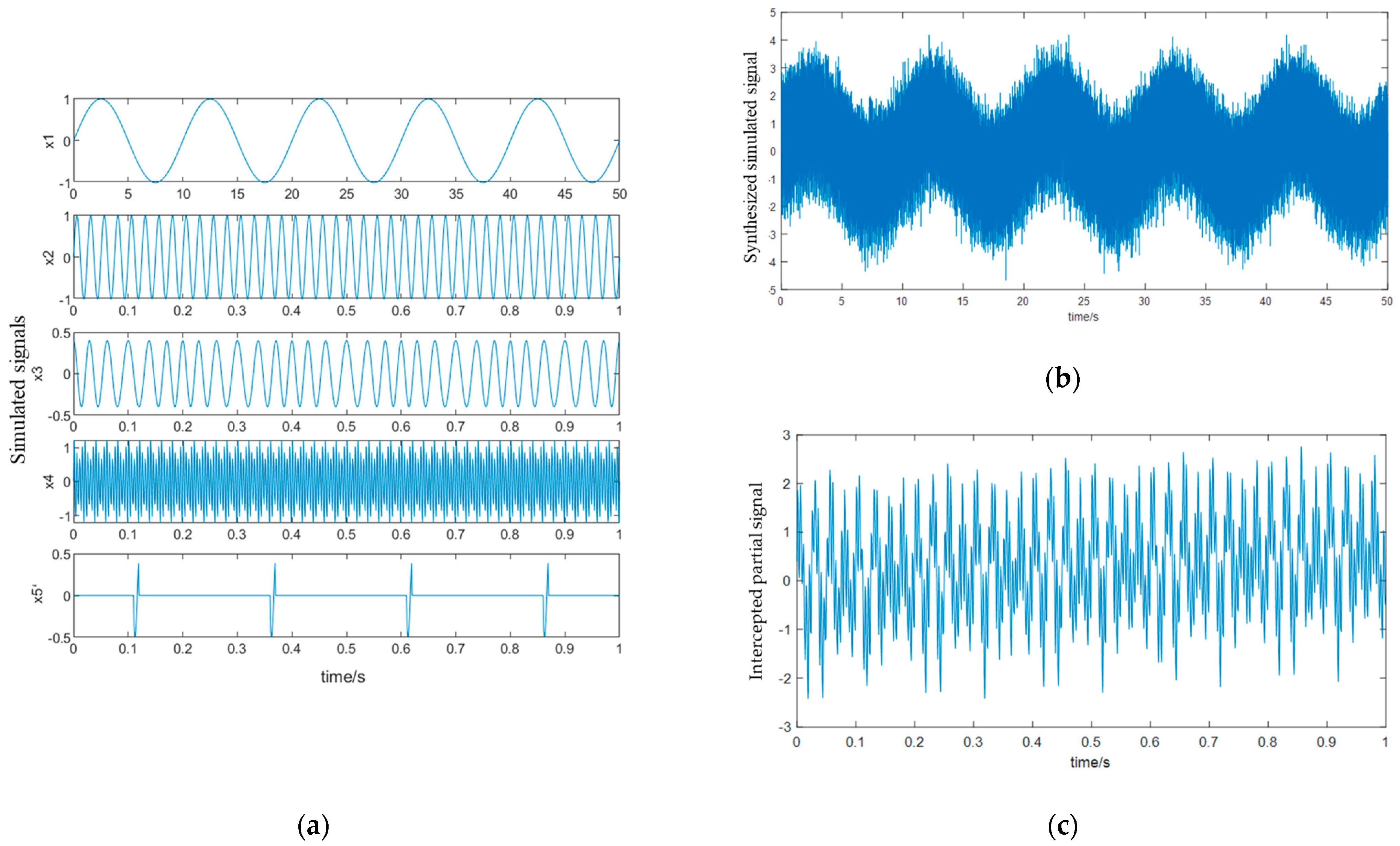
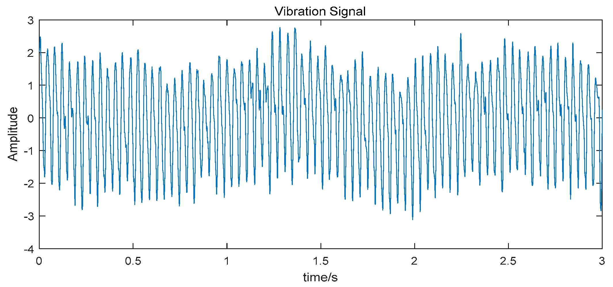
3.1. Artificial Signals

To verify the effectiveness of the proposed method, the performance of ICEEMDAN and other algorithms are compared and analyzed utilizing analog signals synthesized from multiple characteristic signals. The constructed analog signal expressions are as follows:

$$\left\{\begin{array}{l}\begin{array}{l}{x}_1=\sin (0.2\pi t)\\ x_2=\sin (80\pi t)\end{array}\hfill \\ x_3=0.4\cos (60\pi t+\sin (10\pi t))\hfill \\ x_4=\sin (400\pi t)(1+0.3\cos (100\pi t))\hfill \\ x_5=0.5\sin (120\pi t)\hfill \end{array}\right.$$

(5)

where $x_1$ is a low-frequency signal, $x_2$ is a sinusoidal periodic signal, $x_3$ is a frequency-modulated signal, $x_4$ is an amplitude-modulated signal, $x_5$ is a high-frequency sinusoidal signal that is processed to form an intermittent pulse signal $x_5^{\prime }$, as shown in Figure 2a. Also, $\eta$ is an added noise; the above signals are added together to synthesize the simulated signal $x$, as shown in Figure 2b. During the simulation verification, we intercept part of the signal from Figure 2b, as shown in Figure 2c.

$$x=x_1+x_2+x_3+x_4+x_5^{\prime }+\eta$$

(6)

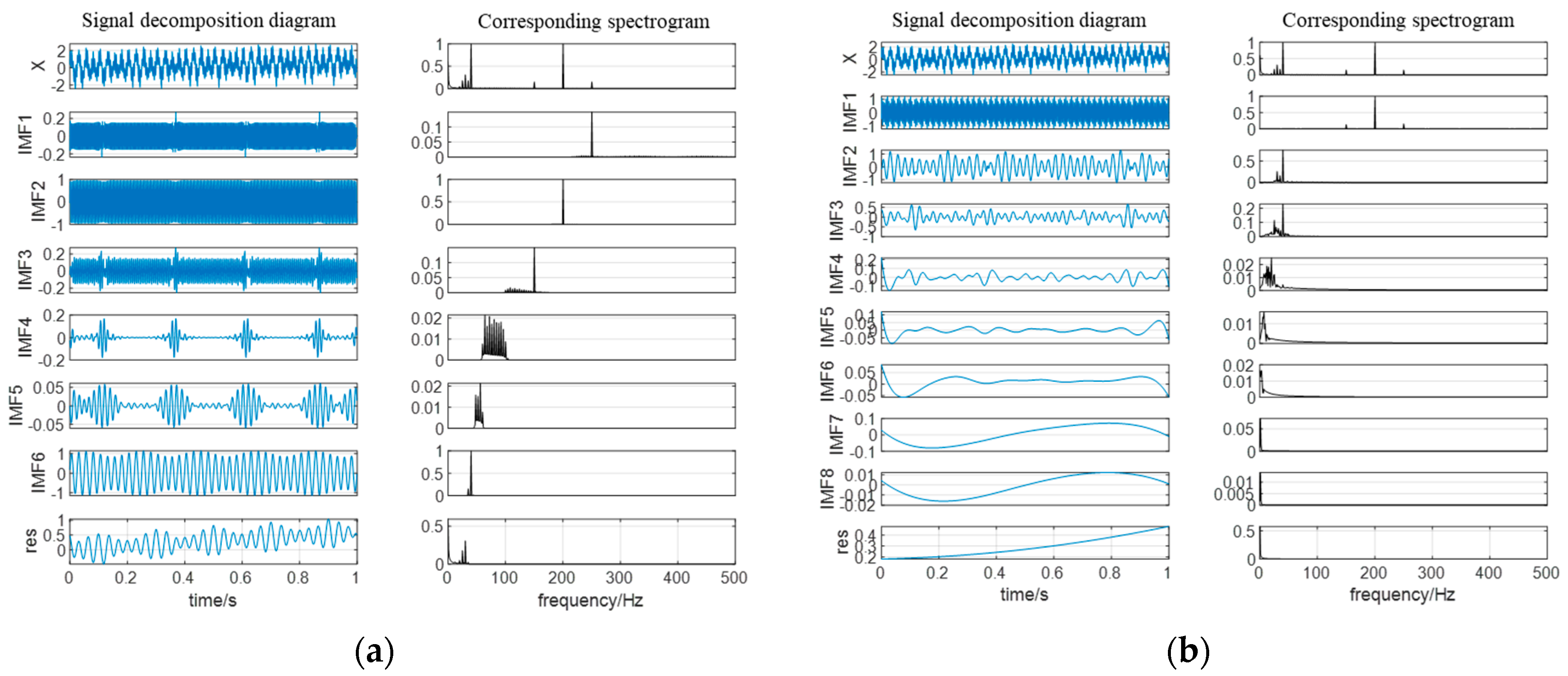
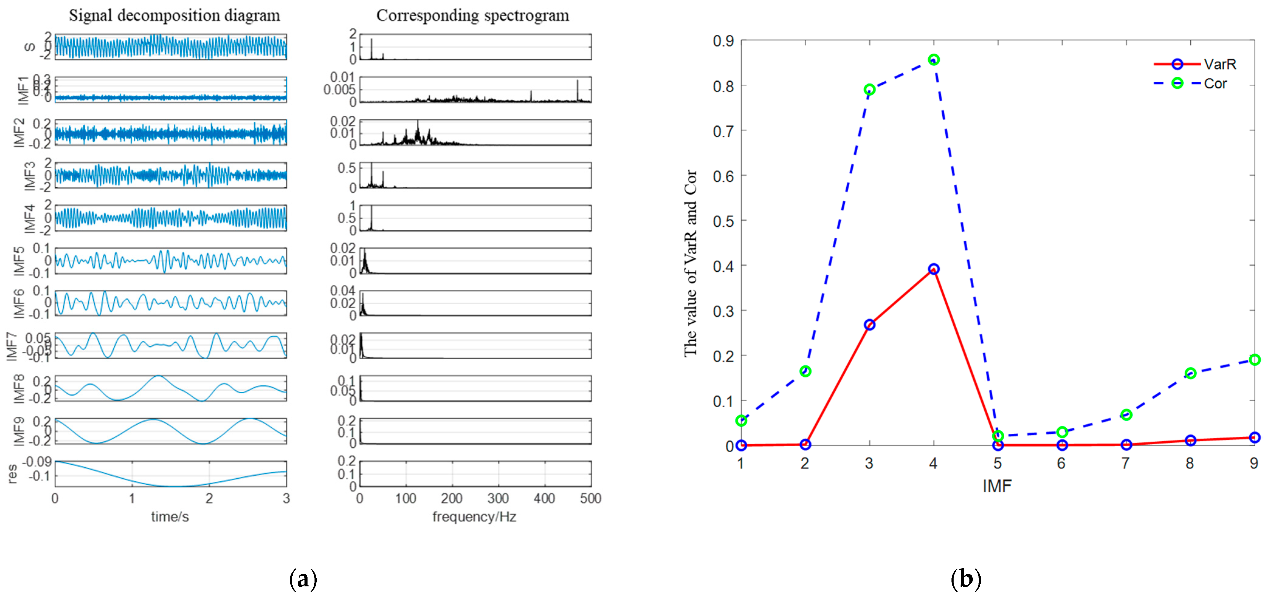
3.2. ICEEMDAN Decomposition Signal Analysis

The empirical mode decomposition (EMD) is proposed by Professor Huang for analyzing non-stationary signals. Its process is essentially a means of smoothing non-stationary signals. The result is a step-by-step decomposition of fluctuations and trends of different scales in the signal, producing a series of data series with different characteristic scales. Handrin et al. [23] used EMD to statistically analyze the results after white noise decomposition and proposed an improved EMD method based on noise-assisted analysis, namely ensemble empirical mode decomposition (EEMD). The complete ensemble empirical mode decomposition with adaptive noise (CEEMDAN) [24] is an improvement from EMD while borrowing the idea of adding Gaussian noise and decomposing the signal by superimposing and averaging multiple times to cancel the noise from the EEMD method. The empirical wavelet transform (EWT) was proposed by Gilles in 2013 [25]. This method is a combination of the EMD method and wavelet transform; the idea is to divide the spectrum of the signal and construct a suitable wavelet filter bank to decompose the signal.

The synthetic signal is decomposed using the EWT, EEMD, CEEMDAN, and ICEEMDAN decomposition methods, where the noise level added by the three noise-assisted empirical mode decomposition methods is 0.2, and the total number of sets is 100. To compare the performance advantages and disadvantages of the four methods in detail, the decomposition results of the four decomposition methods, as well as the related indexes, will be analyzed and compared as follows:

• Comparison of decomposition results. The time-domain and frequency-domain results of each IMF component and residual component (res) obtained using the four decomposition methods are shown in Figure 3. Comparing the decomposition results in Figure 3, we can see that EWT needs to set its maximum decomposition order based on a priori knowledge, and the other three types of EMD methods are all adaptive decomposition, which reduces the subjectivity of human experience. However, there is serious modal confounding between the components obtained by EEMD, while the improved adaptive noise-assisted ICEEMDAN attenuates this modal confounding phenomenon. Meanwhile, EEMD and CEEMDAN decompose more than eight IMF components: EEMD decomposition starts from IMF6, and CEEMDAN decomposition starts from IMF8, and the signal components have very small energy, and these components may be spurious components appearing in the decomposition and do not represent the information of the original signal. In contrast, in the improved adaptive noise-assisted ICEEMDAN decomposition, not only the main frequency components are decomposed, but also only a smaller number of IMF components are decomposed. This is due to its strict adherence to the global stopping criterion of EMD decomposition, in which the decomposition ends once the conditions for stopping the decomposition are met and the entire cycle is stopped.

2.

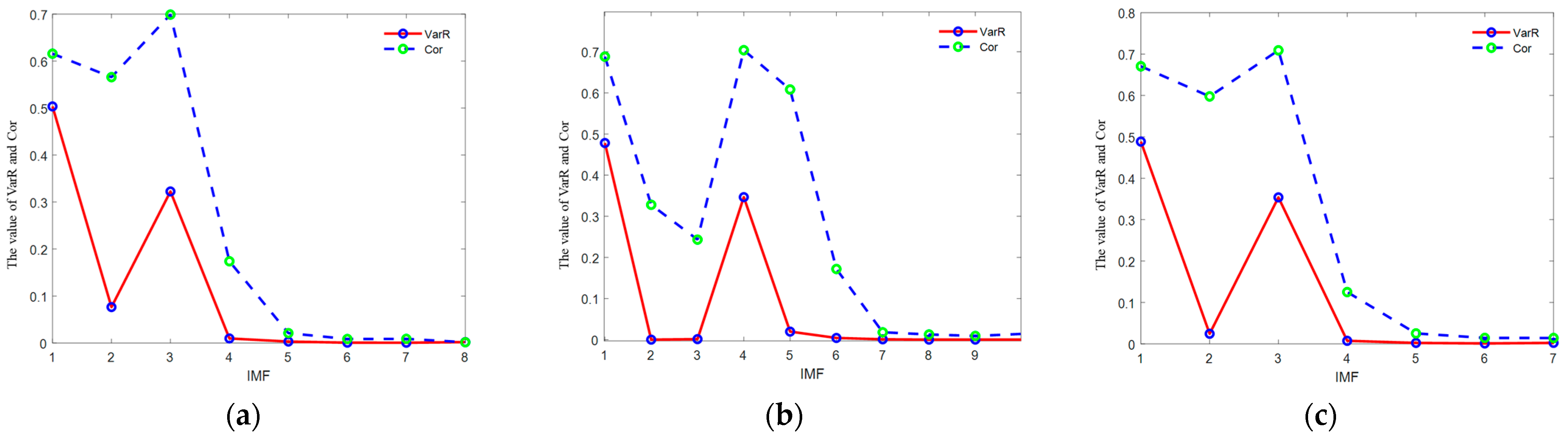
Analysis of the effective IMF component. The signal is decomposed by the above three methods to obtain a set of IMF components that portray different frequency information of the signal respectively, and the frequency distribution information within each IMF component is different, and the variance contribution rate and correlation coefficient of the IMF components obtained by combining the three methods of decomposition in Section 2.2 are calculated as shown in Figure 4, and the validity of the IMF components is analyzed.

As can be seen from Figure 4, where the red solid line represents the variance contribution rate and the blue dashed line represents the correlation coefficient value. The correlation coefficients calculated by the three methods are similar to the overall distribution of the variance contribution rate. In Figure 4c, the correlation coefficients of the first-, second-, and third-order IMF components and the original signal are larger, which indicates that they carry important information about the signal, but the variance contribution rate of IMF2 is smaller, which indicates high noise content, and the correlation and variance contribution rate of the fourth, fifth, and sixth order and the original signal are poor, which indicates serious noise content. To prevent the loss of some details of the signal, we subsequently perform the noise-reduction process for the components with high noise content.

In summary, it can be seen that the ICEEMDAN algorithm does not need to set the maximum decomposition order of EWT, also weakens the modal mixing phenomenon in the EEMD algorithm and CEEMDAN, and also solves the incompleteness drawback; in addition, the ICEEMDAN algorithm has a better correlation coefficient and variance contribution rate. Therefore, the comprehensive performance of the ICEEMDAN algorithm is significantly better than the other three decomposition algorithms.

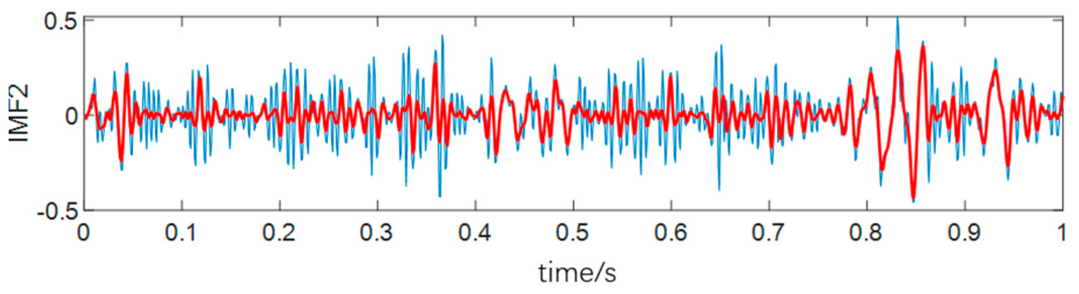
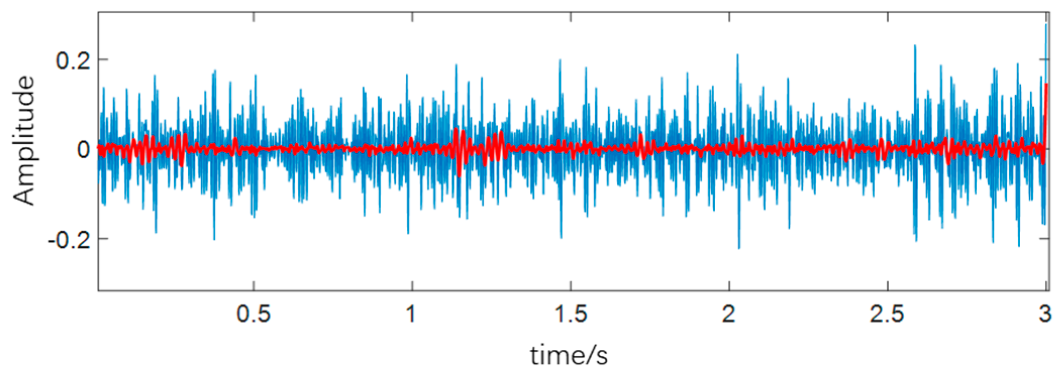
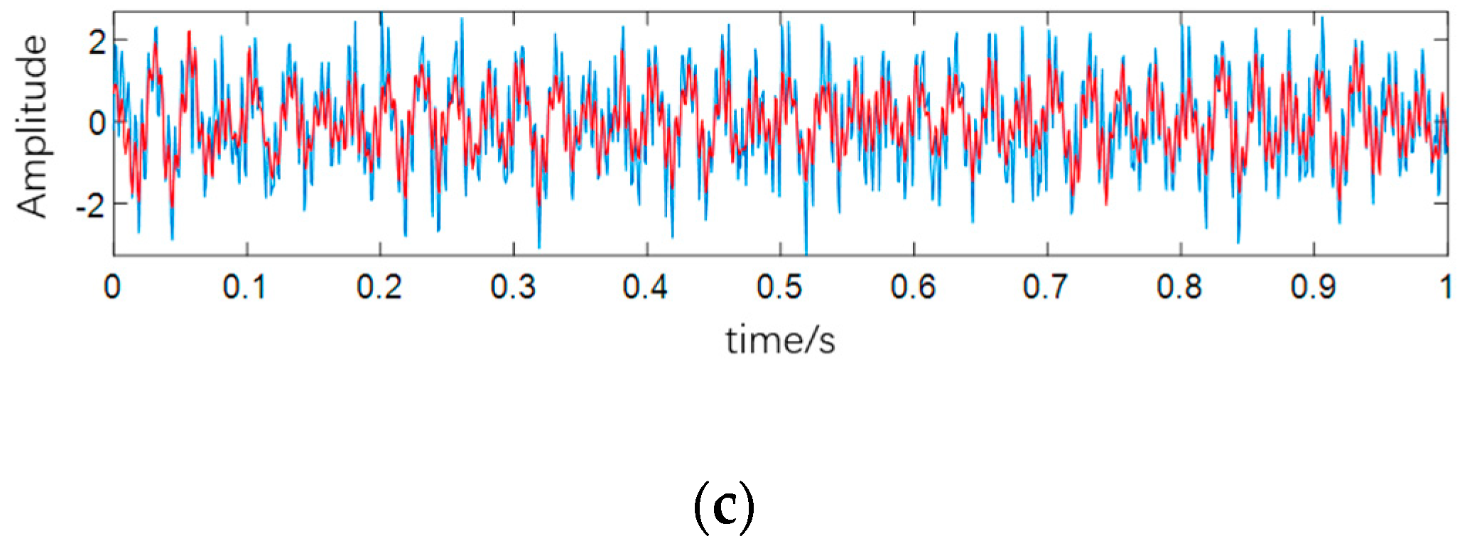
3.3. IMF Component Filtering Analysis

For the selected noise components, we use the LOESS method for noise-reduction processing. In the previous stage, to verify the effectiveness of the LOESS method, we used several filtering and denoising methods for simulated comparison experiments, and the comparison results are shown in Figure 5. Analysis of Figure 5 and its local enlargement, it can be seen that the LOESS method represented by the red curve not only has a good smooth denoising effect on the whole but also has good performance in the local area.

Figure 6 gives the filtering results of the LOESS method for the noise component IMF2 filtered by the ICEEMDAN decomposition. The blue line represents the IMF2 component, and the red line is the signal after noise reduction obtained by the LOESS filtering method. It can be seen that the LOESS filtering method can remove the noise interference well and retain the information in the component.

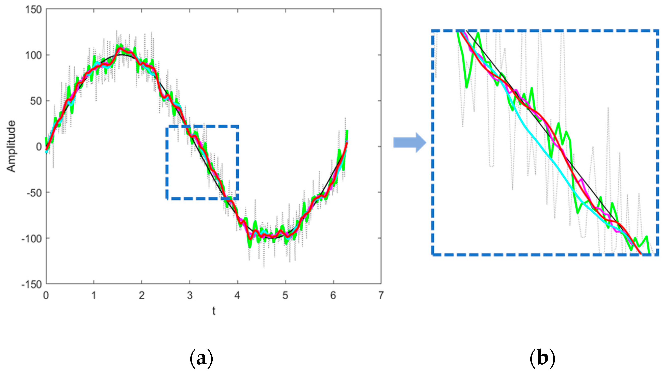
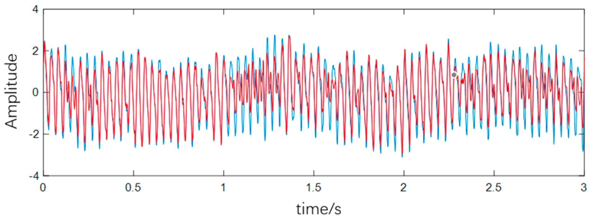
3.4. Evaluation of Results

The signal noise-reduction process aims to filter out unwanted noise from the signal and preserve the useful signal while maintaining the original smoothness and similarity to the pure signal after the noise is removed. This process is important for improving the quality of the signal and ensuring its accuracy. We introduce two noise-reduction discrimination criteria: signal-to-noise ratio (SNR) and root-mean-square error (RMSE) [26].

The signal-to-noise ratio is the ratio of the energy of the useful signal to the noise signal in the signal and is used to evaluate the noise-reduction effect of the signal. The larger the SNR of the signal after noise reduction, the more effective the signal contains useful components, and the smaller the noise components, the better the effect of noise-reduction SNR is calculated by Equation (7).

$$SNR=10\lg \frac{{\displaystyle \sum _{i=1}^N{s}^2(i)}}{{\displaystyle \sum _{i=1}^N{(s(i)-\tilde{s}(i))}^2}}$$

(7)

At the same time, the root-mean-square error is introduced to measure the noise-reduction signal’s deviation from the original signal. RMSE is calculated by the formula; the smaller the value, the smaller the error between the noise-reduction signal and the original signal, and the closer the two signals are, the better the noise-reduction effect.

$$RMSE=\sqrt{\frac{{\displaystyle \sum _{i=1}^N{(s(i)-\tilde{s}(i))}^2}}{N}}$$

(8)

In the above two equations, $s(i)$ is the pure signal, $\tilde{s}(i)$ is the signal with noise (artificial signals), and N is the sampling point of the signal.

The comparison of SNR and root-mean-square error RSME of the three methods is given in

Table 1. Comparison of noise-reduction effect.

	ICEEMDAN +LOESS	CEEMDAN +LOESS	EEMD +LOESS
SNR	12.64	7.73	7.10
RMSE	0.28	0.43	0.46

. The combination of ICEEMDAN and LOESS filtering yields a relatively large SNR and a small root-mean-square error, which illustrates the effectiveness of the methods for signal analysis. Meanwhile, the reconstructed effect graphs obtained by the three types of EMD decomposition methods are shown in Figure 7. It can be seen that the proposed method can not only decompose the signal well but also has obvious advantages over other methods in terms of noise reduction, so the method proposed in this paper can be adapted to process and analyze the vibration signal of marine atomic gravimeters.

4. Vibration Measurement Signal Analysis

To verify the effectiveness of the algorithm in the practical application of the vibration signal of the marine atomic gravimeter, the vibration data of the atomic gravimeter were collected by navigation tests. The measurement system is shown in Figure 8, which mainly consists of an atomic gravimeter and a shipboard inertial stabilization platform accelerometer. The atomic absolute gravimeter is rigidly fixed to the upper part of the shipboard inertial stabilization platform, which is fastened to the ship deck, and the accelerometer is rigidly fixed to the atomic gravimeter to measure the vibration signal.

During the test, the accelerometer converts the collected vibration information into an analog voltage output, and the data collector performs analog-to-digital conversion of the analog signal and transmits the digital information to the computer. The data collection software (Labview 2018) is installed in the computer to store and process the received digital information, and finally, the vibration data of 1000 sampling points are randomly selected for analysis, as shown in Figure 9.

The decomposition analysis of the marine atomic interferometric gravimeter vibration signal is performed using the method proposed in this paper, which is displayed in Figure 10. Figure 10a shows that ICEEMDAN decomposes the measured vibration signal to obtain 10 IMFs, including IMF1–IMF9 and a residual component denoted as res, with a reasonable number of decomposed components; analyzed from top to bottom, IMF1 and IMF2 are the high-frequency index components, and the signals are concentrated above 100 Hz, IMF3–IMF9 are the low-frequency index components, and the signals are concentrated within 0.1–50 Hz. It can be seen that the decomposed components become smoother and smoother, i.e., the component frequencies become lower and lower. The correlation coefficients and variance contributions of each component are calculated in Figure 10b; the correlation coefficients of low-frequency components IMF3 and IMF4 reach 0.8–0.9, and the variance contributions are between 0.3 and 0.4, which are much larger than other components and belong to the effective components. The values of all indicators of IMF1 and IMF5 are relatively small, indicating that they are redundant components and are treated as discarded. The correlation coefficient of IMF2 is higher, and its variance contribution is lower, which is determined to be a noisy component. To further obtain useful detailed vibration information in the noisy component IMF2, the LOESS filter is used for noise reduction, as shown in Figure 11. In the figure, the blue curve represents the untreated IMF2, and the red curve represents the IMF after noise reduction, which shows that the LOESS method is obvious and useful for removing the IMF2 noise.

Finally, the filtered effective components and the processed noise components are reconstructed, and the results are shown in Figure 12, where the blue curve is the original vibration signal, and the red curve is the signal processed by the proposed method, which is consistent with the analysis results of the simulating signal. It shows that the method proposed in this paper can not only decompose the signal well but also reduce the noise of the signal.

In summary, the vibration signal of the atomic gravimeter shows consistency with the theoretical analysis [27,28]. The vibration noise mainly consists of low-frequency band ground pulse noise and a small portion of high-frequency band noise, but it is still primarily concentrated in the low-frequency band (0.1–50 Hz). Meanwhile, the correlation coefficients and variance contributions of the IMFs in the high-frequency band are relatively small, indicating that the information in the high-frequency band is correlated with the original signal and has little influence on the original signal. Therefore, when considering the design of the vibration isolation device for the atomic gravimeter, the vibration isolation device in the lower frequency band will have a better vibration isolation effect to overcome the influence of the ground pulse vibration.

5. Conclusions

Due to the vibration of the surrounding environment and the self-oscillation of the system, the high-precision ocean atomic interferometric gravimeter embodies complex vibration characteristics during the measurement process, which seriously affects the measurement accuracy of the instrument. Based on the existing research techniques, the vibration characteristics of the ocean atomic interferometric gravimeter are analyzed and investigated, and the combination of improved complete ensemble empirical mode decomposition with adaptive noise (ICEEMDAN) and locally weighted regression (LOESS) was proposed. The simulated signals verify that the proposed method can extract different components of complex signals and overcome the phenomenon of modal mixing that exists in other empirical mode decomposition methods, as well as eliminate invalid components. The final SNR metrics and RMSE metrics are better than the other two methods in this paper. In addition, the method in this paper is also effectively verified on the vibration data of the ocean atomic gravimeter, and the time-frequency characteristics of the vibration signals in various frequency bands are obtained, and a good noise-reduction effect is also achieved for the signals. Therefore, this work provides a reference strategy for optimally processing the vibration data of the ocean atomic gravimeter and provides theoretical support for the next step of the subject to design the vibration isolation device of the atomic gravimeter.

References

1. Kasevich, M.; Chu, S. Atomic interferometry using stimulated Raman transitions. Phys. Rev. Lett. 1991, 67, 181–184. [Google Scholar] [CrossRef]
2. Peters, A.; Chung, K.Y.; Chu, S. Measurement of gravitational acceleration by dropping atoms. Nature 1999, 400, 849–852. [Google Scholar] [CrossRef]
3. Tino, G.M. Testing gravity with cold atom interferometry: Results and prospects. Quantum Sci. Technol. 2021, 6, 024014. [Google Scholar] [CrossRef]
4. Taylor, R.G.; Scanlon, B.; Döll, P.; Rodell, M.; Van Beek, R.; Wada, Y.; Longuevergne, L.; Leblanc, M.; Famiglietti, J.S.; Edmunds, M.; et al. Groundwater and climate change. Nat. Clim. Chang. 2013, 3, 322–329. [Google Scholar] [CrossRef]
5. Tapley, B.D.; Bettadpur, S.; Ries, J.C.; Thompson, P.F.; Watkins, M.M. GRACE Measurements of Mass Variability in the Earth System. Science 2004, 305, 503–505. [Google Scholar] [CrossRef]
6. Van Camp, M.; de Viron, O.; Watlet, A.; Meurers, B.; Francis, O.; Caudron, C. Geophysics From Terrestrial Time-Variable Gravity Measurements. Rev. Geophys. 2017, 55, 938–992. [Google Scholar] [CrossRef]
7. Huang, P.W.; Tang, B.; Chen, X.; Zhong, J.Q.; Xiong, Z.Y.; Zhou, L.; Wang, J.; Zhan, M.S. Accuracy and stability evaluation of the 85Rb atom gravimeter WAG-H5-1 at the 2017 International Comparison of Absolute Gravimeters. Metrologia 2019, 56, 045012. [Google Scholar] [CrossRef]
8. Yang, R.; Song, Z.; Chen, L.; Gu, Y.; Xi, X. Assisted cold start method for GPS receiver with artificial neural network-based satellite orbit prediction. Meas. Sci. Technol. 2020, 32, 015101. [Google Scholar] [CrossRef]
9. Bajpai, R.; Tomaru, T.; Yamamoto, K.; Ushiba, T.; Kimura, N.; Suzuki, T.; Yamada, T.; Honda, T. A laser interferometer accelerometer for vibration sensitive cryogenic experiments. Meas. Sci. Technol. 2022, 33, 085902. [Google Scholar] [CrossRef]
10. Hinton, A.; Perea-Ortiz, M.; Winch, J.; Briggs, J.; Freer, S.; Moustoukas, D.; Powell-Gill, S.; Squire, C.; Lamb, A.; Rammeloo, C.; et al. A portable magneto-optical trap with prospects for atom interferometry in civil engineering. Philos. Trans. R. Soc. A Math. Phys. Eng. Sci. 2017, 375, 20160238. [Google Scholar] [CrossRef] [PubMed]
11. Gabor, D. Theory of communication. Part 1: The analysis of information. Electrical Engineers Part III Radio & Communication. Eng. J. Inst. 1946, 93, 429–441. [Google Scholar]
12. Mallat, S.A. Theory for multi-resolution signal decomposition wavelet representation. IEEE Trans. Pattern Anal. Mach. Intell. 1989, 11, 674–693. [Google Scholar] [CrossRef]
13. Huang, N.E.; Shen, Z.; Long, S.R.; Wu, M.C.; Shih, H.H.; Zheng, Q.; Yen, N.C.; Tung, C.C.; Liu, H.H. The empirical mode decomposition and the Hilbert spectrum for nonlinear and non-stationary time series analysis. Proc. R. Soc. Lond. A 1998, 454, 903–995. [Google Scholar] [CrossRef]
14. Tang, B.P.; Jiang, Y.H.; Zhang, X. Feature extraction method of rolling bearing fault based on singular value decomposition-morphology filter and empirical mode decomposition. J. Mech. Eng. 2010, 46, 37–42. [Google Scholar] [CrossRef]
15. Zhang, J.; Sang, H.; Zhao, S. EMD-based time–frequency denoising algorithm for the self-sensing of vibration signals in ultrasonic-assisted grinding. Meas. Sci. Technol. 2022, 33, 104004. [Google Scholar] [CrossRef]
16. Zhong, C.; Wang, J.S.; Sun, W.Z. Fault diagnosis method of rotating bearing based on improved ensemble empirical mode decomposition and deep belief network. Meas. Sci. Technol. 2022, 33, 085109. [Google Scholar] [CrossRef]
17. Zhou, X.Y.; Ji, Z.; Wang, F.W. Short-term ship traffic flow prediction based on EEMD-PE-LSTM and visualization of channel traffic state. J. Dalian Marit. Univ. 2023, 49, 58–68. [Google Scholar]
18. Yang, Z.Z.; Lin, J.Z.; Wang, K. De-noising of concrete acoustic emission signals based on CEEMD-wavelet packet adaptive threshold. J. Vib. Shock 2023, 42, 139–149. [Google Scholar]
19. Lo, A.W.; MacKinlay, C. The size and power of the variance ratio test in finite samples. J. Econ. 1989, 40, 203–238. [Google Scholar] [CrossRef]
20. Fisher, R.A.S.; Bennett, J.H. Statistical Methods, Experimental Design, and Scientific Inference; Oxford University Press: Oxford, UK, 1990. [Google Scholar]
21. Fisher, R. On the ‘probable error’ of a coefficient of correlation deduced from a small sample. Metron 1920, 1, 3–32. [Google Scholar]
22. Cui, C.R. A study on the parameterization of mesoscale wind stress induced feedback effect and its role in reducing the simulated SST warm bias in the western coast of South America. Inst. Oceanol. Chin. Acad. Sci. Univ. Chin. Acad. Sci. 2021, 39, 785–799. [Google Scholar]
23. Wu, Z.; Huang, N.E. Ensemble empirical mode decomposition: A noise-assisted data analysis method. Adv. Adapt. Data Anal. 2009, 1, 1–41. [Google Scholar] [CrossRef]
24. Torres, M.E.; Colominas, M.A.; Schlotthauer, G.; Flandrin, P. A complete ensemble empirical mode decomposition with adaptive noise. In Proceedings of the IEEE International Conference on Acoustics, Speech and Signal Processing, Prague, Czech Republic, 22–27 May 2011; pp. 4144–4147. [Google Scholar]
25. Gilles, J. Empirical wavelet transform. IEEE Trans. Signal Process. 2013, 61, 3999–4010. [Google Scholar] [CrossRef]
26. Trevor, H.; Robert, T.; Jerome, F. The Elements of Statistical Learning; Springer Press: Berlin/Heidelberg, Germany, 2009. [Google Scholar]
27. Yao, J.M.; Wu, K.; Guo, M.Y. An Ultralow-frequency active vertical vibration isolator with geometric anti-spring structure for absolute gravimetry. IEEE Trans. Instrum. Meas. 2020, 69, 2670–2677. [Google Scholar] [CrossRef]
28. Hu, R.; Wu, S.Q.; Mou, Z.L.; Feng, J.Y.; Niu, X.B. Vibration characteristics of absolute gravimeter. J. Vib. Meas. Diagn. 2022, 42, 220–226+403. [Google Scholar]
Figure 1. Vibration-signal analysis process.
Jmse 12 00302 g001
Figure 2. Artificial signals: (a) simulated signals; (b) synthesized simulated signal; and (c) intercepted partial signal.
Jmse 12 00302 g002
Figure 3. Decomposition results and corresponding spectrograms by four methods of decomposing the simulated signal x. The left column shows the IMF of each component of the signal after decomposition for each method, and the right column shows the spectrogram corresponding to each IMF component: (a) EWT, (b) EEM, (c) CEEMDAN, and (d) ICEEMDAN.
Jmse 12 00302 g003aJmse 12 00302 g003b
Figure 4. Correlation coefficients and variance contribution values of each IMF for different methods. (a) EEMD, (b) CEEMDAN, and (c) ICEEMDAN.
Jmse 12 00302 g004
Figure 5. (a) Comparison of the smoothing results of several filtering methods; (b) the local enlargement. The black dotted line is the input data, the black solid line is the sine, the green line is mean filtered data, the magenta line is Savitzky–Golay filtered data, the cyan line is RLOESS filtered data, and the red line is LOESS filtered data.
Jmse 12 00302 g005
Figure 6. Filtering results of LOESS method for noise component IMF2: the blue line represents the IMF2 (non-denoised signal), and the red line is the signal after noise reduction.
Jmse 12 00302 g006
Figure 7. Reconfiguration effects of three different methods: the blue curves represent the un-noised reconstructed signals, and the red curves represent the reconstructed signals after denoising. (a) EEMD; (b) CEEMDAN; (c) ICEEMDAN.
Jmse 12 00302 g007aJmse 12 00302 g007b
Figure 8. Marine atomic gravimeter measurement experiment system.
Jmse 12 00302 g008
Figure 9. Vibrational signals from the Atomic Ocean Gravimeter.
Jmse 12 00302 g009
Figure 10. ICEEMDAN decomposition analysis: (a) the left column shows the signal map IMF for each component of the ICEEMDAN decomposition, and the right column shows the spectrogram corresponding to each IMF component; (b) the correlation coefficients and variance contributions corresponding to each IMF.
Jmse 12 00302 g010
Figure 11. The filtering effect of the LOESS method on the noise component IMF2: the blue curve represents the untreated IMF2, and the red curve represents the IMF after noise reduction by the LOESS method.
Jmse 12 00302 g011
Figure 12. Reconstruction of the resulting map: the blue curve is the original vibration signal, and the red curve is the reconstructed signal after processing by the proposed method.
Jmse 12 00302 g012