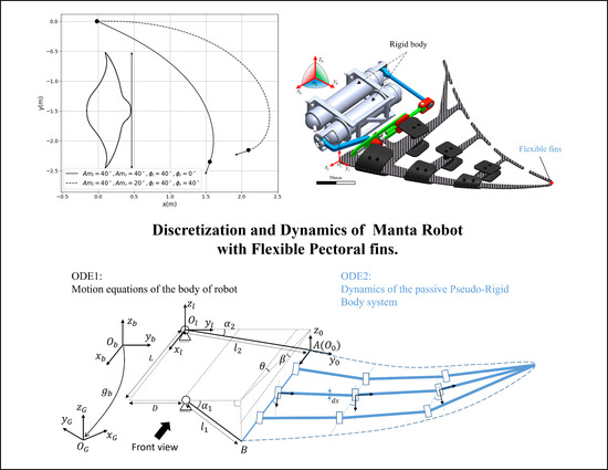
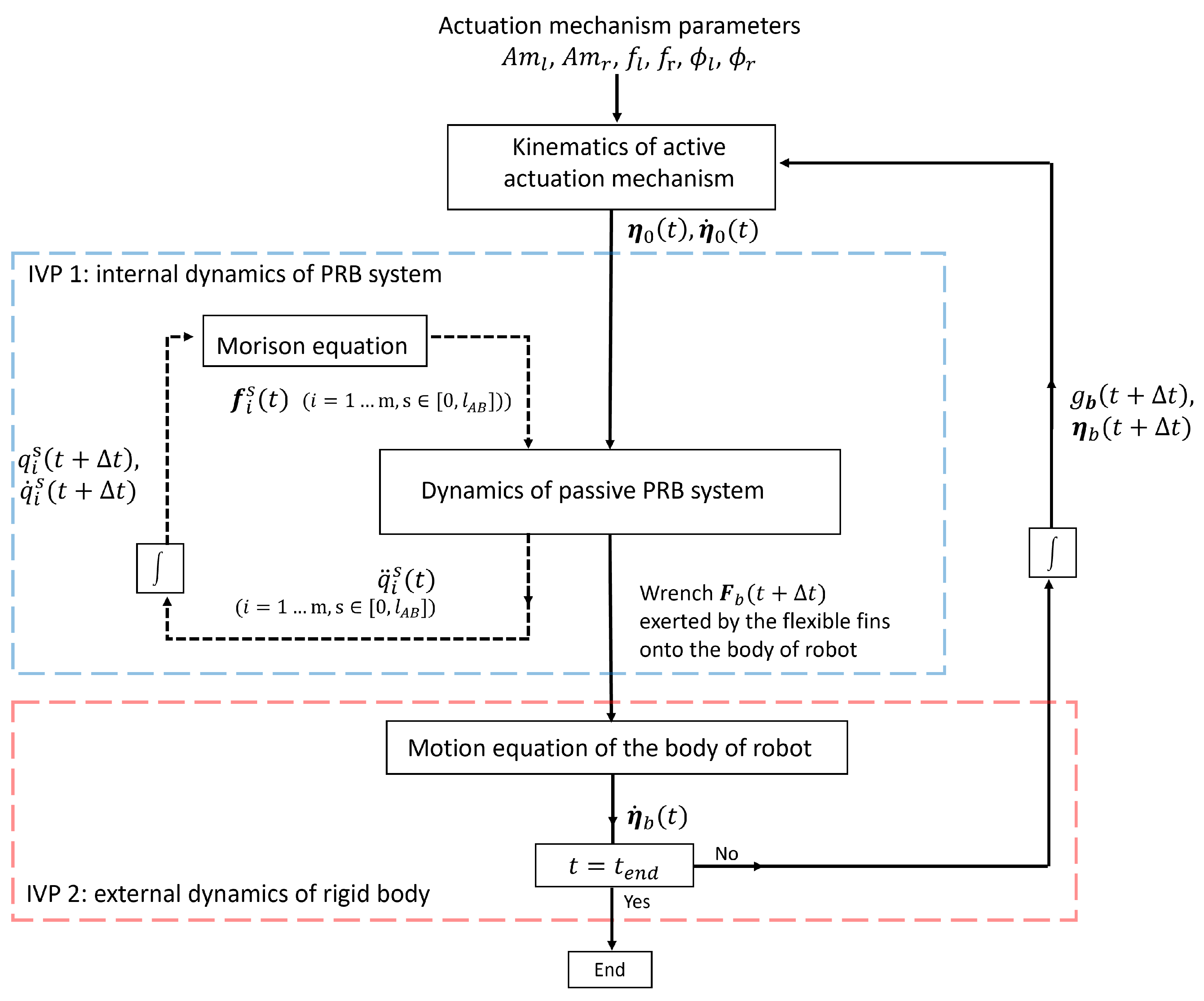
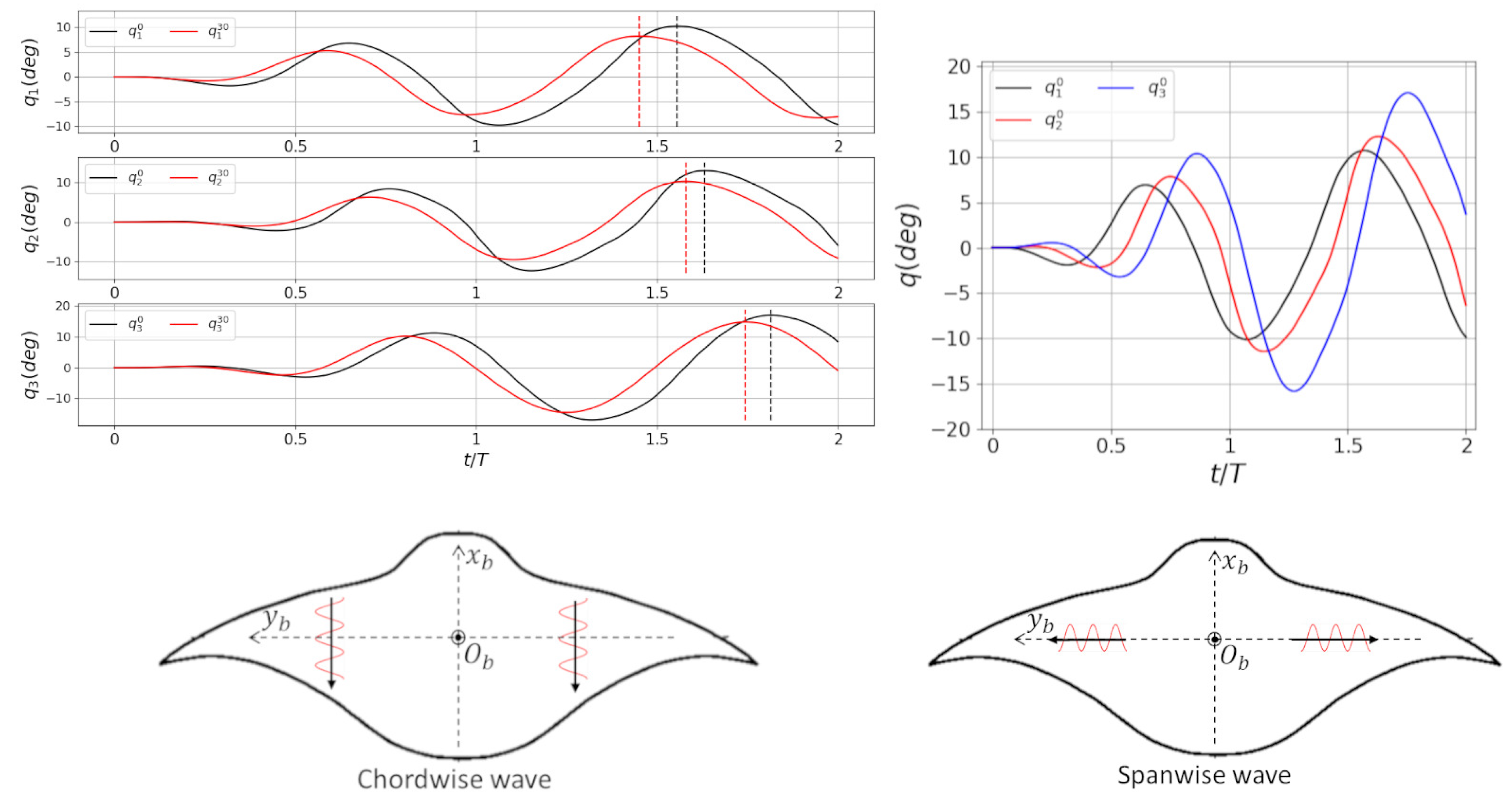
A Rigid-Flexible Coupling Dynamic Model for Robotic Manta with Flexible Pectoral Fins

Abstract

The manta ray, exemplifying an agile swimming mode identified as the median and paired fin (MPF) mode, inspired the development of underwater robots. Robotic manta typically comprises a central rigid body and flexible pectoral fins. Flexible fins provide excellent maneuverability. However, due to the complexity of material mechanics and hydrodynamics, its dynamics are rarely studied, which is crucial for the advanced control of robotic manta (such as trajectory tracking, obstacle avoidance, etc.). In this paper, we develop a multibody dynamic model for our novel manta robot by introducing a pseudo-rigid body (PRB) model to consider passive deformation in the spanwise direction of the pectoral fins while avoiding intricate modeling. In addressing the rigid-flexible coupling dynamics between flexible fins and the actuation mechanism, we employ a sequential coupling technique commonly used in fluid-structure interaction (FSI) problems. Numerical examples are provided to validate the MPF mode and demonstrate the effectiveness of the dynamic model. We show that our model performs well in the rigid-flexible coupling analysis of the manta robot. In addition to the straight-swimming scenario, we elucidate the viability of tailoring turning gaits through systematic variations in input parameters. Moreover, compared with finite element and CFD methods, the PRB method has high computational efficiency in rigid-flexible coupling problems. Its potential for real-time computation opens up possibilities for future model-based control.

1. Introduction

1.1. Manta Robot

Bionic underwater robots have presented several desired properties, gradually becoming a rapidly evolving research area in recent years [1,2]. Unlike ordinary underwater vehicles, these bio-inspired robots achieve propulsion through the undulating motion of their flexible bodies and fins. This mode of motion demonstrates a novel concept for transferring energy that relies on the motion and elastic deformation of flexible members’ interaction directly with fluid. According to the swimming mode, they can be generally divided into two categories. Robots utilizing the body and/or caudal fin (BCF) mode [3] typically have narrow and flexible bodies, upon which they rely to generate strong propulsion for high swimming speeds. In contrast, those adopting the median and/or paired fin (MPF) mode [4] are characterized by the flapping motion of their broad pectoral fins. Manta ray is typical of the MPF mode, exhibiting efficient and agile swimming characteristics. With the powerful flapping of huge fins, they can forage at a speed of 0.25–0.47 m/s [5]. The wing-like fins endow the manta ray with bird-like high maneuverability and pitch capability as well as remarkable. Inspired by the skeleton structure of the pectoral fin of mantas, our group has developed a novel prototype of robotic manta with carbon fiber flexible pectoral fins driven actively by a space six-link mechanism [6]. We have experimentally demonstrated that with the flexible fins, the prototype can reproduce the passive oscillations and wave transmissions of the mantas, resulting in outstanding hydrodynamic performance. In this study, we aim to build a dynamic model of this prototype to describe the passive deformation of the flexible fins under fluid-structure interaction, in order to establish a relation between the 3D motion of the robot and the parameters of fin motion.

1.2. Commonly Used Theories and Methods for Modeling Manta Robot

With the development of robotic manta, dynamic modeling indicates a significant role. Indeed, accurate and efficient models can be used to not only predict and analyze the behavior of robots in complex environments but also develop model-based design and control. A convenient approach in modeling a robotic manta is to decompose it into a series of linkage mechanisms. In this case, the manta robot is considered a typical mobile rigid multibody system. The commonly valid assumption is that the structure of the flexible fins is composed of a series of rigid links attached by compliant joints [7,8].

The locomotion dynamics of mobile multibody systems can be obtained by the Lagrangian formulation based on the Euler-Lagrange equation. Indeed, although the Lagrangian formulation is a powerful tool for dynamic modeling, it is not suited for complex hyper-redundant continuous or discrete systems [9]. Hence, in our study, we chose to use the Newton-Euler Dynamics Algorithm (NEDA) based on the Newton-Euler formulation. Due to its ease of implementation and high computational efficiency, NEDA is widely used in the modeling of bio-inspired locomotors [10]. In the recent literature, the fins of a robotic manta are divided into a series of motion-determined crank-rocker mechanisms to characterize their rigid motion [11]. We have also noticed that most NEDA is used to characterize the hydrodynamics by quasi-steady hydrofoil theory [12], also known as the Morison equations. Systematic comparisons between the simulations and experiments show that the method can predict the robot’s essential features, such as the velocity, attitude, and body oscillation within a wide range of control parameters [13,14].

Besides, pioneering researchers also explore how to consider passive deformation via various beam theories to provide more precise results on simple hydrodynamic problems. Lighthill’s elongated body theory [15] or large-amplitude elongated body theory [16] are widely accepted methods for modeling robotic fish via a continuum method. For instance, Boyer et al. [17] simulated the 2-D locomotion of an eel-like robot by using a Cosserat rod model, which considers elemental quasi-static lift and drag. These methods balance fidelity and simplicity well but are only available for planar locomotion. By solving the Navier-Stokes equation, the 3D distribution of hydrodynamic forces can be computed through Computational Fluid Dynamics (CFD) simulations, where the robot can be modeled as a fully flexible continuum via beam, shell, or solid element [18,19]. However, this computationally expensive approach is not amenable to designing a controller for the robot.

As for the overall multibody system modeling, it has been extensively studied in the context of underwater snake robots [20], but the dynamics model specifically for the manta robot remains scarce. Not limited to the modeling of underwater snake robots, there are approximately four main modeling families for soft robotics: geometric models, continuum mechanics models, discrete models, and data-driven models [21]. Geometric models replace the skeleton with different geometric shapes [22], while continuum mechanics models most commonly utilize finite element models [23]. Both of them face challenges in reducing dimensions for real-time simulations [21]. Data-driven models are physics-agnostic approaches that can be possibly applied to any design and scenario [24]. However, the resulting models are not generalizable to new designs and conditions. In dealing with different robots with flexible parts, we can distinguish discrete models into the following three main groups: the lumped-mass [25], the Pseudo-Rigid-Body [26], and the discrete rods models [27]. They are widely used for underwater robots because of allowing real-time simulation. However, they are more commonly applied in one-dimensional cases, and there are fewer systematic papers about a robotic manta. The modeling of the MPF mode with flexible fins still requires more comprehensive and unified research.

Essentially, modeling the hydrodynamics via the flexible fins of the manta robot is about simultaneously accounting for the passive deformation of the flexible fins while maintaining a high computational efficiency. We can adopt the mobile rigid multibody and Morison equations as the main framework because they benefit the construction of 3-D motions and effectively balance fidelity and simplicity. To describe passive deformation within the same framework, we utilize Pseudo-Rigid-Body Models (PRBMs) [28], which introduce elastic deformation between discrete rigid links. This involves applying a set of springs to each joint to characterize the deflected deformation, simulating behavior like an Euler-Bernoulli beam. Furthermore, the flexible fins coupling with rigid motion will be considered using a sequential-coupling technique [29].

1.3. Structure of the Paper

In this paper, we first remind the basic definitions and notations of rigid multibody mechanics in Section 2. In Section 3, we adopt the model of mobile multibody systems to derive a general unified framework devoted to the modeling of locomotion and, in particular, bio-inspired locomotion of our robotic manta. It consists of the dynamics of pectoral fins based on the PRB model, the dynamics of the rigid body of the robot, and the hydrodynamics introduced through the Morison equation. Then, the numerical method based on NEDA will be introduced in Section 4. The pectoral fins and the body of the robot are sequentially coupled. The following Section 5 and Section 6 deal with numerical validation and conclusion. Various motion gaits of the manta robot will be achieved through our simulations. In all these developments, the constitutive bodies of the robots are considered discrete, rigid bodies with flexible joints, presenting a modeling framework for robotic manta with flexible pectoral fins.

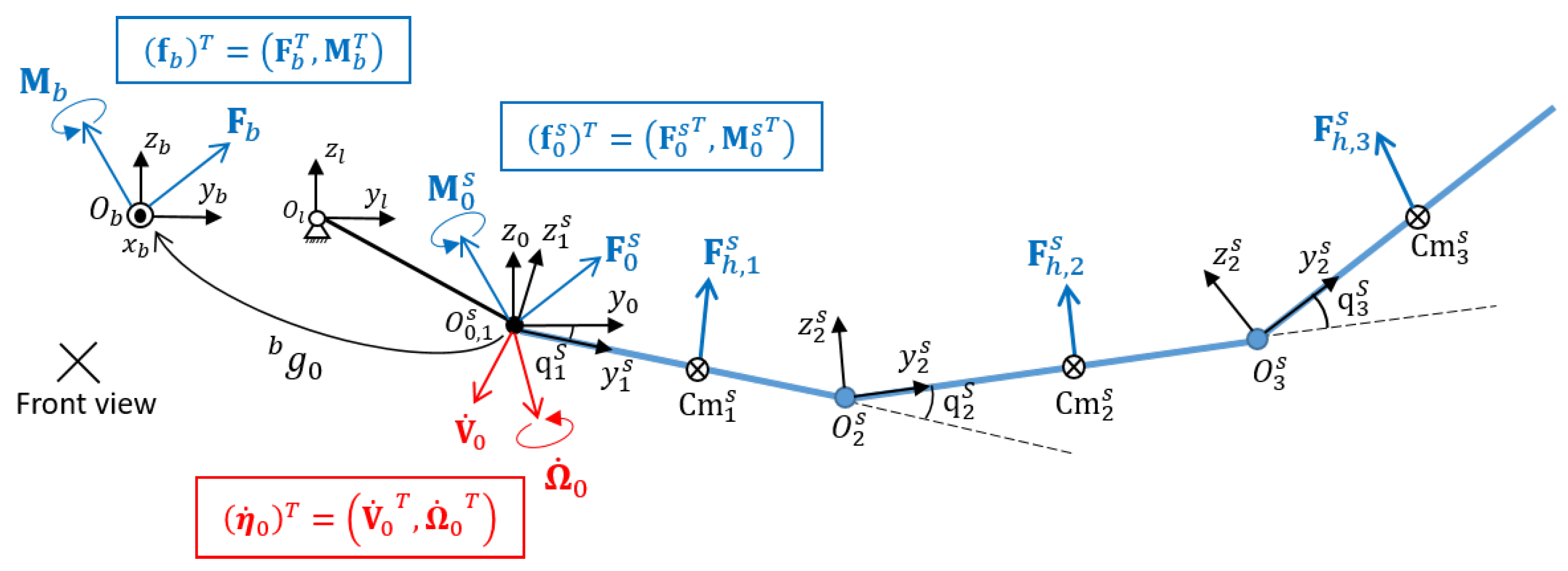
2. Basic Definitions and Notations of Rigid Multibody Mechanics

The modeling of mobile multibody systems involves both relative motions between rigid bodies and overall rigid-body motion in space. The transformations applied to a rigid body can be represented by $4\times 4$ homogeneous matrices of the form:

$${\mathbf{g}}_0=\left(\begin{array}{cc}{\mathbf{R}}_{\mathbf{0}}& {\mathbf{p}}_0\\ {\mathbf{0}}_{1\times 3}& 1\end{array}\right)\in {\mathbb{R}}^{(4\times 4)}$$

(1)

where ${\mathbf{R}}_{\mathbf{0}}$ is a $3\times 3$ rotation matrix (i.e., an element of $SO\left(3\right)$), and ${\mathbf{p}}_0$ is a translation vector. Geometrically, the matrix $\mathbf{g}$ defines the pauses of a mobile frame attached to the body with respect to a fixed inertial frame ${\mathcal{F}}_G$ (Figure 1), and more abstractly, points on the non-commutative Lie group $SE\left(3\right)$. The adjoint representation of the configuration matrix is defined with an operator “Ad”

$${\mathrm{Ad}}_{{\mathbf{g}}_j}=\left(\begin{array}{cc}{R}_j& {\hat{p}}_j{R}_j\\ 0_{3\times 3}& R_j\end{array}\right)$$

(2)

where a widehat “$\widehat{\left(\right)}$” converts ${\mathbb{R}}^3$ in $so\left(3\right)$.

Throughout the article, a transformation ${\left({}^{j-1}\mathbf{g}_j\right)}^k$ represents the position of j-th rigid body w.r.t. the fixed coordinate frame ${\mathcal{F}}_{j-1}$ of $(j-1)$-th rigid body in the k-th serial chain. Therefore, the transformation matrix of j-th rigid body is described as:

$${\left({\mathbf{g}}_j\right)}^k={\mathbf{g}}_0{\left({}^0\mathbf{g}_1\right)}^k{\left({}^1\mathbf{g}_2\right)}^k\dots {\left({}^{j-1}\mathbf{g}_j\right)}^k$$

(3)

with the right subscript indicating the index of the related body and the left and right superscript indicating respectively the index of the projection frame and the index of the serial chain.

The velocities of a rigid body define the Lie algebra of $SE\left(3\right)$, denoted by $se\left(3\right)$, which is represented by the space of twists, i.e., by $6\times 1$ vectors ${\mathit{\eta }}_0^T=\left({\mathbf{V}}_0^T,{\Omega }_0^T\right)$ composed of an angular component ${\Omega }_0$ (angular velocity) and a linear one ${\mathbf{V}}_0$ (linear velocity). We introduced the operator “ad”, defined for any $6\times 1$ vectors, by the $6\times 6$ matrix:

$${\mathrm{ad}}_{{\mathit{\eta }}_j}=\left(\begin{array}{cc}{\hat{\Omega }}_j& {\hat{\mathbf{V}}}_j\\ {\mathbf{0}}_{3\times 3}& {\hat{\Omega }}_j\end{array}\right)$$

(4)

where a hat “ $^$ ” covering a vector $\mathbf{Y}$ defines a matrix $\hat{\mathbf{Y}}$ whose definition depends on the dimension of $\mathbf{Y}$. If $\mathbf{Y}=\Omega \in {\mathbb{R}}^3$, $\hat{\Omega }$ denotes the unique $3\times 3$ skew-symmetric matrix of $\Omega$. If $\mathbf{Y}=\mathit{\eta }\in {\mathbb{R}}^6$, $\hat{\mathit{\eta }}$ is the unique $4\times 4$ matrix defined by:

$$\hat{\eta }=\left(\begin{array}{cc}\hat{\Omega }& \mathbf{V}\\ {\mathbf{0}}_{1\times 3}& 0\end{array}\right)$$

(5)

All the expressions of the article can be interpreted as matrix relations in terms of components in the mobile basis of the body frames.

3. Dynamic Modeling

The modeling of the prototype can be divided into two parts: the central robot body and the symmetrical flexible pectoral fins. In the following section, the central body is considered as a rigid body, of which the base frame ${\mathcal{F}}_b$ is fixed on its mass center $O_b$. Therefore, the configuration matrix from the base frame to frame ${\mathcal{F}}_G$ is described as $g_b$. The flexible pectoral fin will be described as a multi-rigid-body linkage mechanism combined with passively deformable structures connected to the base. The manta robot will be regarded as a typical mobile multibody system.

The schematic representation of the pectoral fin mechanism is illustrated in Figure 2. In terms of describing the fin mechanism of the manta robot, the actuation mechanism is simplified into two parallel rods driven by motors (black part of Figure 2). The endpoints A and B of the rod are connected by a support attached by a succession of serial pseudo-rigid bodies (blue part of Figure 2). For the sake of simplicity of dynamic modeling, we omit all the inertia effects of the actuation mechanism and assume that the motors can produce exactly the desired rod oscillations.

3.1. Kinematics of the Active Actuation Mechanism of Fins

We start with the kinematic model of the active actuation mechanism, allowing us to calculate the velocity and acceleration of the support AB with a fixed length L. The motion of the support will be used to drive the flexible fins in the following Section 3.3.

Taking the fin on the left side as an example, the frame ${\mathcal{F}}_l=\left(O_l{x}_b{y}_l{z}_l\right)$ fixed on the motor of the backward rod (see Figure 2) parallel to the body frame ${\mathcal{F}}_b$. $\theta$ represents the angle between $x_b{o}_b{z}_b$ and the projection of $l_{AB}$ on $x_b{o}_b{y}_b$, and $\beta$ represents the angle between $l_{AB}$ and $x_b{o}_b{y}_b$. Knowing the velocity ${\mathit{\eta }}_b={({\mathbf{V}}_b^T,{\Omega }_b^T)}^T$ and the acceleration of body ${\dot{\mathit{\eta }}}_b={({\dot{\mathbf{V}}}_b^T,{\dot{\Omega }}_b^T)}^T$ of body with respect to the global frame ${\mathcal{F}}_G$, we obtain the velocity twist ${\mathit{\eta }}_l$ and the acceleration twist ${\dot{\mathit{\eta }}}_l$ of the origin $O_l$ by the relation

$$\left\{\begin{array}{c}{\mathbf{V}}_l={\mathbf{V}}_b+{\Omega }_b\times {}^b\mathbf{P}_l\hfill \\ {\Omega }_l={\Omega }_b\hfill \\ {\dot{\mathbf{V}}}_l={\dot{\mathbf{V}}}_b+{\dot{\Omega }}_b\times {}^b\mathbf{P}_l\hfill \\ {\dot{\Omega }}_l={\dot{\Omega }}_b\hfill \end{array}\right.$$

(6)

with ${}^b\mathbf{P}_l$ the fixed position vector of origin $O_l$ in the frame ${\mathcal{F}}_b$.

By denoting the endpoint A of the backward rod as the point $O_0$, the frame of the support AB is determined by ${\mathcal{F}}_0$. The position vector of the origin $O_0$ in ${\mathcal{F}}_l$ is given by

$${}^l\mathbf{P}_0={(0,l_{2}cos\left({\alpha }_2\right),l_{2}sin\left({\alpha }_2\right))}^T$$

(7)

The relative rotation matrix ${}^{l}R_0$ is determined by two Euler angles $\theta$ and $\beta$ as functions of ${\alpha }_1$, ${\alpha }_2$ (see details in [6]), such that

$${}^{l}R_0={}^{l}R_{\overline{0}}\left(\theta \right){}^{\overline{0}}R_0\left(\beta \right)$$

(8)

with the matrices ${}^{l}R_{\overline{0}}\left(\theta \right)$, ${}^{\overline{0}}R_0\left(\beta \right)$ describing respectively two rotations, given by

$${}^{l}R_{\overline{0}}\left(\theta \right)=\left(\begin{array}{ccc}cos\left(\theta \right)& -sin\left(\theta \right)& 0\\ sin\left(\theta \right)& cos\left(\theta \right)& 0\\ 0& 0& 1\end{array}\right),{}^{\overline{0}}R_0\left(\beta \right)=\left(\begin{array}{ccc}cos\left(\beta \right)& 0& sin\left(\beta \right)\\ 0& 1& 0\\ -sin\left(\beta \right)& 0& cos\left(\beta \right)\end{array}\right)$$

(9)

The velocity and acceleration of the origin $O_0$ are given by

$$\left\{\begin{array}{c}{\mathbf{V}}_0={}^{0}R_l\left({\mathbf{V}}_l+({\Omega }_l+\dot{{\alpha }_2}\mathbf{x})\times {}^l\mathbf{P}_0\right)\hfill \\ {\Omega }_0={}^{0}R_l{\Omega }_l+{}^{0}R_{\overline{0}}\dot{\theta }\mathbf{z}+\dot{\beta }\mathbf{y}\hfill \\ {\dot{\mathbf{V}}}_0={\dot{\mathbf{V}}}_l+({\dot{\Omega }}_l+{\ddot{\alpha }}_2\mathbf{x})\times {}^l\mathbf{P}_0\hfill \\ {\dot{\Omega }}_0={}^{0}R_l{\dot{\Omega }}_l+{}^{0}R_{\overline{0}}\left({\Omega }_{\overline{0}}\times \dot{\theta }\mathbf{z}\right)+{}^{0}R_{\overline{0}}\ddot{\theta }\mathbf{z}+{\Omega }_0\times \dot{\beta }\mathbf{y}+\ddot{\beta }\mathbf{y}\hfill \end{array}\right.$$

(10)

where $\mathbf{x},\mathbf{y},\mathbf{z}$ are respectively the unit vectors ${(1,0,0)}^T,{(0,1,0)}^T,{(0,0,1)}^T$, the derivatives $\dot{\theta },\dot{\beta },\ddot{\theta },\ddot{\beta }$ are formulized in [6]. The velocity of a certain point $s\in [0,L]$ on the support, denoted by $({\mathbf{V}}_0^s,{\Omega }_0^s)$, is calculated by the relations ${\mathbf{V}}_0^s={\mathbf{V}}_0+{\Omega }_0\times s\mathbf{x}$ and ${\Omega }_0^s={\Omega }_0$. This velocity is associated also with the first node of the PRB system, input as an initial condition to solve its dynamics.

3.2. Morison Hydrodynamic Forces

In the preceding section, we have obtained the velocity and acceleration transfer matrix for the flexible fins. Subsequently, we can calculate the hydrodynamic forces of each link of PRB system expressed in its local frame (${\mathcal{F}}_j^s=O_j^s,x_j^s,y_j^s,z_j^s$) using the Morison equation, as this equation is solely dependent on the velocity and direction vectors of the structure as shown in Figure 3. The normal vector ${\mathbf{n}}_j^s$ defined by the corresponding nodes of one serial chain can be estimated as follows:

$${\mathbf{n}}_j^s={\mathbf{Cm}}_j^s\times ({\mathbf{R}}_j^s+{\mathbf{E}}_j^s)$$

(11)

where ${\mathbf{Cm}}_j^s$ represents the coordinates of the midpoint of the link (⊗ in Figure 3), ${\mathbf{R}}_j^s$ and ${\mathbf{E}}_j^s$ ($j=1,2,3$) is tangent to the shape curve (red dashed line) in the chordwise direction of the fins [11]. Here, we assume that, when the discretization width $ds$ of the link tends towards 0, the tangents ${\mathbf{R}}_j^s$ and ${\mathbf{E}}_j^s$ can be considered as the line connecting the origins $O_j^s$, $O_j^{s-1}$ of two adjacent links (black dashed line). The calculation of the tangents therefore requires the coordinates of the origin $O_j^{s-1}$ expressed in the frame ${\mathcal{F}}_j^s$, which can be obtained by the relation (3). The vector ${\mathbf{n}}_j^s$ is normalised such that ${\mathbf{n}}_j^s\mapsto ({\mathbf{n}}_j^s/|{\mathbf{n}}_j^s\left|\right)$.

The hydrodynamic forces that result from the interaction of the MMS (Mobile Multibody System) and fluid can be determined using Morison’s Equation, which combines an inertial term and a drag term. The drag term can be further divided into the tangential force and the normal force. Since the flexible film is lightweight and the liquid is viscous, only the normal force is considered in the hydrodynamic model [30]. The hydrodynamic force on a single link $\left(j\right)$ can be formulated as:

$${\mathbf{F}}_{h,j}^s=-\frac{1}{2}\rho C_{D,j}{∥{\mathbf{V}}_{\mathrm{cm},j}^s{\mathbf{n}}_j^s∥}^2·{\mathbf{n}}_j^{s}d{S}_j$$

(12)

where ${\mathbf{F}}_{h,j}^s$, $\rho$, $C_{D,j}$, $d{S}_j$ represent the hydrodynamic force exerted onto the midpoint ${\mathrm{Cm}}_j^s$, the density of water, the drag coefficient and the cross-sectional area along the motion direction. Since the links are homogeneous and rigid, the midpoint ${\mathrm{Cm}}_j^s$ represents also its center of gravity. The linear velocity ${\mathbf{V}}_{\mathrm{cm},j}^s$ is obtained by the same velocity transfer in Section 3.1 and will not be reiterated here. We denote that the force ${\mathbf{F}}_{h,j}^s$ is expressed in the local frame ${\mathcal{F}}_j^s$ to solve the dynamics of PRB system in the next section.

3.3. Dynamics of Passive PRB System

This section deals with the dynamic modeling of the flexible pectoral fins based on the framework of the mobile multibody system [9]. Yun et al. established the dynamic model of a manta robot with MPF mode for the first time [11]. The robot’s fins are flexible films driven by two parallel rigid linkages. The motion of rigid linkages predetermines the motions of the flexible films without considering any inertia effects. For our robot, however, the actuation mechanism is located at the base of the flexible fins (see Figure 2). It’s thus difficult to estimate directly the motion of the flexible fins through that of the actuation mechanism. The challenge here is to couple the rigid motions of driving linkages and the dynamics of the passive flexible fins to describe both the internal motion (flexible fins) and the external motion (rigid body) of the system.

Many approaches are applied to model the passive deformation of different robots, such as finite element methods [31] or CFD methods [32]. These methods involve resolving partial differential equations (PDE) with complex boundary conditions. In our study, the soft material system of fins is discretized as a tree-like mass-spring-damping system (or PRB system). The evolution of this system is described by ordinary differential equations (ODE), capturing the physical properties of flexible fins, such as bending stiffness, material damping, and inertial effects. The establishment of ODE is based on a Newton-Euler recursive algorithm, which is applied by Boyer et al. [7,8] for the first time to model the flexible flapping wings of a flying insect-like robot. The advantage of this algorithm is that it integrates the dynamics of the redundant structure of the robot in a concise and rapid way.

Based on the work of Boyer et al., we made two improvements to the Newton-Euler algorithm (detailed respectively in Section 3.3.1 and Section 3.3.2), to adapt the physical properties of flexible fins. On the one hand, the bending torque of each passive joint in [8] is calculated by a linear viscous-elastic model. Here, to better describe the elastic deformation of the flexible fin, the bending torque is calculated from an energetic point of view; on the other hand, for the flapping wing, each serial chain of the tree-like structure has only one passive revolute joint. In our study, we extend the serial chains of the PRB system to any number of DoFs. The benefit of doing so is to better describe the deformation of the slander structure, thereby generating the spanwise waves necessary for propulsion.

One serial chain of the PRB system with three DoFs is illustrated in Figure 4. The NEDA consists of two parts. The first is to calculate the joint accelerations ${\ddot{\mathbf{q}}}^s={({\ddot{q}}_1^s,{\ddot{q}}_2^s,{\ddot{q}}_3^s)}^T$ through the velocity ${\mathit{\eta }}_0^s$ and acceleration ${\dot{\mathit{\eta }}}_0$ of the actuation mechanism obtained in Section 3.1 and the hydrodynamic force ${\mathbf{F}}_{h,1}^s$ exerted onto each passive link obtained in Section 3.2. The accelerations ${\ddot{\mathbf{q}}}^s$ are used to update the motion state (${\mathbf{q}}^s,{\dot{\mathbf{q}}}^s$) of the tree-like PRB system in the next time step. The second is to calculate the wrench ${\left({\mathbf{f}}_0^s\right)}^T=({{\mathbf{F}}_0^s}^T,{{\mathbf{M}}_0^s}^T)$ exerted onto the base of each serial PRB linkage, which integrates the inertial, damping, and hydrodynamic effects. These wrenches are transferred to the body frame ${\mathcal{F}}_b$ and integrated as the resultant wrench ${\left({\mathbf{f}}_b\right)}^T=({{\mathbf{F}}_b}^T,{{\mathbf{M}}_b}^T)$ exerted the fin on the body, used to solve the dynamics of the rigid body of robot in the next section. The details of NEDA are introduced in Section 3.3.2.

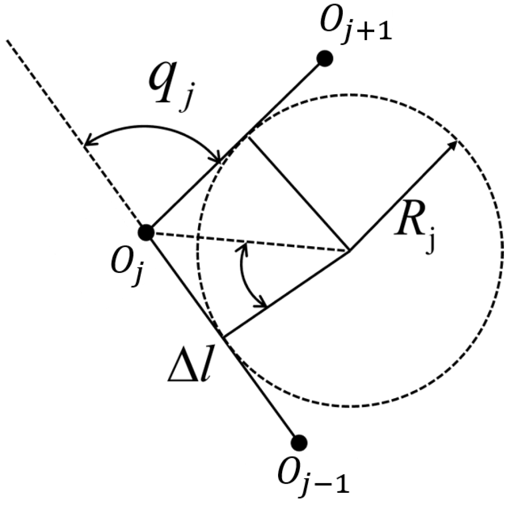
3.3.1. Elastic Bending Forces

As the deformation of the fins remains in 2D, we do not include a twisting energy of the rod, although this can be readily integrated into our framework. The link between two consecutive nodes is rigid. The turning angle $q_j$ (see Figure 5) at node $O_j$ between two attached links can produce a nonlinear resorting torque, similar to a torsional spring. The elastic energy from the strains in the fins can be represented by the linear sum of the bending energy associated with variation in the turning angle at the nodes, which is:

$$E_j=\frac{1}{2}EI{(k_j-{\overline{k}}_j)}^2\Delta l$$

(13)

where $EI$ is the bending stiffness, $k_j=2\tan (q_j/2)/\Delta l$ is the curvature (Figure 5), and ${\overline{k}}_j$ is the natural curvature, which is zero in this study.

The elastic bending forces acting on a node $O_j$ can be obtained from the gradient of the energies:

$${\tau }_{j,e}=-\frac{\partial E_j}{\partial q_j}$$

(14)

A node $O_j$ is only coupled with the adjacent nodes $O_{j-1}$ and $O_{j+1}$ in the discrete energy formulation. The equilibrium equations in the body-fixed coordinates can be established for each joint.

In addition to the internal elastic forces, the structure would also undergo internal damping forces during deformation, which are associated with a damping coefficient c as defined in [33]:

$${\tau }_{j,d}=-c_j\dot{q_j}$$

(15)

3.3.2. Detailed Newton-Euler Dynamic Algorithm

We present here the detailed Newton-Euler Dynamics Algorithm (NEDA) for solving the dynamics of a single series chain of passive PRB system with m DoF. At a certain moment t, the joint position ${\mathbf{q}}^s\left(t\right)$ and velocity ${\dot{\mathbf{q}}}^s\left(t\right)$ and the velocity ${\mathit{\eta }}_0^s\left(t\right)$ and the acceleration ${\dot{\mathit{\eta }}}_0^s\left(t\right)$ of the origin $O_0^s\left(t\right)$ are known. The problem consists of computing the joint acceleration ${\ddot{\mathbf{q}}}^s\left(t\right)$ and the wrench ${\mathbf{f}}_0^s\left(t\right)$ exerted by the first link of the PRB system onto the origin $O_0^s\left(t\right)$. For the sake of simplicity, the superscript “s” is omitted in this section.

Based on the N-E formulation, the recursive inverse dynamics is composed of one forward and one backward recursive loop. In this process, three recursive equations are applied in the loops. At first, from the first link to the last m-th link, the velocity ${\mathit{\eta }}_j$ and the acceleration ${\dot{\mathit{\eta }}}_j$ of each link are calculated by the following equations:

$${\mathit{\eta }}_j={{{\mathrm{Ad}}_j}_g}_{j-1}{\mathit{\eta }}_{j-1}+{\mathbf{A}}_j{\dot{q}}_j$$

(16)

$${\dot{\mathit{\eta }}}_j={{{\mathrm{Ad}}_j}_g}_{j-1}{\dot{\mathit{\eta }}}_{j-1}+{\mathit{\zeta }}_j+{\mathbf{A}}_j{\ddot{q}}_j$$

(17)

for $j\in [1,2,\dots ,m]$, with ${\mathbf{A}}_j={({\mathbf{0}}_3^T,{\mathbf{e}}_j^T)}^T$ where ${\mathbf{e}}_j=(1,0,0)$ the unit vector along the j-th joint axis in our study. ${{{\mathrm{Ad}}_j}_g}_{j-1}$ represents the adjoint representation of relative configuration ${}^{j}g_{j-1}$ (see Equation (2)). The term ${\mathit{\zeta }}_j$ stands the time derivative of the adjoint representation and reads ${\mathit{\zeta }}_j={\mathrm{ad}}_{{\eta }_j}{\mathbf{A}}_j{\dot{q}}_j\in {\mathbb{R}}^6$ (see Equation (4)).

By applying Newton’s law and Euler’s theorem to the j-th link, its dynamic equations are expressed in a backward recursive form such that

$$\begin{array}{c}{\mathbf{f}}_j-{\mathrm{Ad}}_{{j+1}_{g_j}}^T{\mathbf{f}}_{j+1}+{\mathbf{f}}_{ext,j}={\mathcal{M}}_j{\dot{\mathit{\eta }}}_j+{\mathit{\beta }}_j({\mathit{\eta }}_j,{\dot{q}}_j)\hfill \end{array}$$

(18)

with ${\mathbf{f}}_j$ the wrench exerted by the $(j-1)$-th link onto the j-th link at the origin $O_j$, ${\mathit{\beta }}_j({\mathit{\eta }}_j,{\dot{q}}_j)$ the Coriolis and centrifugal forces and ${\mathcal{M}}_j$ the inertia matrix of j-th link (see [8,17]). The external wrench ${\mathbf{F}}_{ext,j}$ combines the hydrodynamic, elastic bending, and damping forces and forces (see Equations (12), (14) and (15)), given by

$${\mathbf{f}}_{ext,j}=\left(\begin{array}{c}{\mathbf{F}}_{h,j}\\ {\mathbf{Cm}}_j\times {\mathbf{F}}_{h,j}+({\tau }_{j,e}+{\tau }_{j,d}){\mathbf{e}}_j\end{array}\right)$$

(19)

with ${\mathbf{F}}_{h,j}$ the hydrodynamic force and ${\mathbf{Cm}}_j$ the coordinates of center of mass (see Section 3.2). Here, we assume that the density of mass of the links is equal to that of water, and due to its homogeneity, the gravity and the buoyancy cancel each other out.

Before explaining the details of two loops, we can already identify the difficulty of the problem, that there are several unknown terms in Equations (17) and (18), such as the wrenches ${\mathbf{f}}_j$, ${\mathbf{f}}_{j+1}$ and acceleration ${\mathit{\eta }}_j$ in Equation (18). Thus, the first forward recursive consists in computing the relative configuration ${}^{j+1}g_j$ and the velocity ${\mathit{\eta }}_j$. Then acceleration-independent terms, such as ${\mathit{\zeta }}_j$ and ${\mathit{\beta }}_j$ in Equations (17) and (18), are calculated.

The goal of the second backward recursion is to calculate the joint acceleration ${\ddot{q}}_j$, in other words, to calculate ${\mathit{\eta }}_j$ by applying Equations (17) and (18). To do so, one begins from the Newton–Euler equations of the last (or m-th) link, which is not attached by any forward body, taking the following form

$${\mathbf{f}}_m={\mathcal{M}}_m{\dot{\mathit{\eta }}}_m+{\mathit{\beta }}_m-{\mathbf{f}}_{ext,m}$$

(20)

Here, by replacing ${\mathbf{f}}_m$ of N-E equations of $(m-1)$-th link by the relation (20), the inertia and the Coriolis and centrifugal forces of m-th link are cascaded to $(m-1)$-th link, such that

$${\mathbf{f}}_{m-1}={\mathcal{M}}_{m-1}{\dot{\mathit{\eta }}}_{m-1}+{\mathit{\beta }}_{m-1}-{\mathbf{f}}_{ext,m-1}+{{\mathrm{Ad}}_m}_{g_{m-1}}({\mathcal{M}}_m{\dot{\mathit{\eta }}}_m+{\mathit{\beta }}_m-{\mathbf{f}}_{ext,m})$$

(21)

By substituting Equation (17) in Equation (21), one obtain the generalised NE equations with the unknown terms ${\mathbf{f}}_{m-1}$, ${\dot{\mathit{\eta }}}_{m-1}$ and ${\ddot{q}}_m$:

$${\mathbf{f}}_{m-1}={\mathcal{M}}_{m-1}^{*}{\dot{\mathit{\eta }}}_{m-1}+{\mathit{\beta }}_{m-1}^{*}+\mathrm{Ad}_{m_{g_{m-1}}}^T{\mathcal{M}}_m^{*}{\mathbf{A}}_m{\ddot{q}}_m$$

(22)

with the new generalized inertia ${\mathcal{M}}_{m-1}^{*}$ given by

$${\mathcal{M}}_{m-1}^{*}={\mathcal{M}}_{m-1}+\mathrm{Ad}_{m_{g_{m-1}}}^T{\mathcal{M}}_m^{*}\mathrm{Ad}_{m_{g_{m-1}}}$$

(23)

and the generalized wrench ${\mathit{\beta }}_{m-1}^{*}$ given by

$${\mathit{\beta }}_{m-1}^{*}={\mathit{\beta }}_{m-1}-{\mathbf{f}}_{ext,m-1}+\mathrm{Ad}_{m_{g_{m-1}}}^T{\mathcal{M}}_m^{*}{\mathit{\zeta }}_m+\mathrm{Ad}_{m_{g_{m-1}}}^T\left({\mathit{\beta }}_m-{\mathbf{f}}_{ext,m}\right)$$

(24)

By repeating the above process from the last link to the first link, the generalized NE equations of j-th link are constructed [34,35], given by

$${\mathbf{f}}_j={\mathcal{M}}_j^{*}{\dot{\mathit{\eta }}}_j+{\mathit{\beta }}_j^{*}+\sum _{i=j+1}^m\mathrm{Ad}_{i_{g_j}}^T{\mathcal{M}}_i^{*}{\mathbf{A}}_i{\ddot{q}}_i$$

(25)

for $j\in [1,\dots ,m]$, with the generalized inertia and wrench defined by the following recursive relation:

$$\begin{array}{cc}\hfill & \mathrm{if}j=m,\hfill \\ \hfill & \left\{\begin{array}{c}{\mathcal{M}}_j^{*}={\mathcal{M}}_j\hfill \\ {\mathcal{M}}_j^{*}={\mathit{\beta }}_j-{\mathbf{f}}_{ext,j}\hfill \end{array}\right.\hfill \\ \hfill & \mathrm{if}j=1,\dots ,m-1,\hfill \\ \hfill & \left\{\begin{array}{c}{\mathcal{M}}_j^{*}={\mathcal{M}}_{m-1}+\mathrm{Ad}_{{j+1}_{g_j}}^T{\mathcal{M}}_{j+1}^{*}\mathrm{Ad}_{{j+1}_{g_j}}\hfill \\ {\mathit{\beta }}_j^{*}={\mathit{\beta }}_j-{\mathbf{f}}_{ext,j}+\mathrm{Ad}_{{j+1}_{g_j}}^T\left({\mathit{\beta }}_{j+1}^{*}+{\mathcal{M}}_{j+1}^{*}{\mathit{\zeta }}_{j+1}\right).\hfill \end{array}\right.\hfill \end{array}$$

(26)

Here, by cascading the recursive acceleration transmission (17) from the first link to the j-th link, the acceleration ${\dot{\mathit{\eta }}}_j$ is deduced as a function of the given acceleration ${\dot{\mathit{\eta }}}_0$ and the joint accelerations $\dot{\mathbf{q}}$, given by

$${\dot{\mathit{\eta }}}_j=\mathrm{Ad}_{j{g}_0}{\dot{\mathit{\eta }}}_0+\sum _{i=1}^j\mathrm{Ad}_{j{g}_i}{\mathit{\zeta }}_i+\sum _{i=1}^j\mathrm{Ad}_{j{g}_i}{\mathbf{A}}_i{\ddot{q}}_i$$

(27)

By substituting Equation (27) in Equation (25), one obtains a relation between the wrench ${\mathbf{f}}_j$ and the joint acceleration $\ddot{\mathbf{q}}$. Knowing that the passive revolute joints provide no torque along their rotation axis, there is a constraint for each joint, i.e., ${\mathbf{A}}_j^T{\mathbf{f}}_j=0$. Hence, by projecting the generalised NE Equation (25) onto the rotation axis, one obtains m equations of $\ddot{\mathbf{q}}\in {\mathbb{R}}_m$, given by:

$$\begin{array}{c}{\mathbf{A}}_j^T{\mathcal{M}}_j^{*}{\sum }_{i=1}^j\mathrm{Ad}_{j{g}_i}{\mathbf{A}}_i{\ddot{q}}_i+{\mathbf{A}}_j^T{\sum }_{i=j+1}^m\mathrm{Ad}_{i{g}_j}^T{\mathcal{M}}_i^{*}{\mathbf{A}}_i{\ddot{q}}_i=\hfill \\ -{\mathbf{A}}_j^T{\mathcal{M}}_j^{*}\mathrm{Ad}_{j{g}_0}{\dot{\mathit{\eta }}}_0-{\mathbf{A}}_j^T{\mathcal{M}}_j^{*}{\sum }_{i=1}^j\mathrm{Ad}_{j{g}_i}{\mathit{\zeta }}_i-{\mathbf{A}}_j^T{\mathit{\beta }}_j^{*}\hfill \end{array}$$

(28)

for $j\in [1,\dots ,m]$. The left side of Equation (28) associates with the inertia effect of the PRB system and the right side, for its part, represents the torque exerted onto the j-th rotation axis, including the elastic bending torque, the hydrodynamic effect, and the centrifugal and Coriolis effects. The dynamics of the PRB system is thus deduced as a general Lagrangian form, given by

$$\mathbf{M}\ddot{\mathbf{q}}=\mathbf{Q}$$

(29)

Note that the j-th component of the generalized vector $\mathbf{Q}\in {\mathbb{R}}^m$ associates to the right side of Equation (28). By sorting out the left side of Equation (28), the positive definite symmetric inertia matrix $M\in {\mathbb{R}}^{m\times m}$ takes the following form

$$\mathbf{M}=\left(\begin{array}{cccc}{\mathbf{A}}_1^T{\mathcal{M}}_1^{*}{\mathbf{A}}_1& {\mathbf{A}}_1^T\mathrm{Ad}_{2g_1}^T{\mathcal{M}}_2^{*}{\mathbf{A}}_2& \dots & {\mathbf{A}}_1^T\mathrm{Ad}_{m{g}_1}^T{\mathcal{M}}_m^{*}{\mathbf{A}}_m\\ {\mathbf{A}}_2^T{\mathcal{M}}_2^{*}\mathrm{Ad}_{2g_1}{\mathbf{A}}_1& {\mathbf{A}}_2^T{\mathcal{M}}_2^{*}{\mathbf{A}}_2& \dots & {\mathbf{A}}_2^T\mathrm{Ad}_{m{g}_2}^T{\mathcal{M}}_m^{*}{\mathbf{A}}_m\\ ⋮& ⋮& \ddots & ⋮\\ {\mathbf{A}}_m^T{\mathcal{M}}_m^{*}\mathrm{Ad}_{m{g}_1}{\mathbf{A}}_1& {\mathbf{A}}_m^T{\mathcal{M}}_m^{*}\mathrm{Ad}_{m{g}_2}{\mathbf{A}}_2& \dots & {\mathbf{A}}_m^T{\mathcal{M}}_m^{*}{\mathbf{A}}_m\end{array}\right)$$

(30)

So far, the dynamics of the PRB system has been solved. The joint accelerations $\ddot{\mathbf{q}}$ calculated for updating the state of the flexible fins. Moreover, from Equation (25), the wrench exerted by the first link onto the origin $O_0$ is expressed in the following form

$${\mathbf{f}}_0=-\mathrm{Ad}_{1g_0}^T{\mathbf{f}}_1$$

(31)

with

$${\mathbf{f}}_1={\mathcal{M}}_1^{*}{\dot{\mathit{\eta }}}_1+{\mathit{\beta }}_1^{*}+\sum _{i=2}^m\mathrm{Ad}_{i{g}_1}^T{\mathcal{M}}_i^{*}{\mathbf{A}}_i{\ddot{q}}_i$$

(32)

The wrench exerted by the flexible fin onto the center of mass of the robot, denoted by ${\mathbf{f}}_b$, is thus calculated by the following spatial integration

$${\mathbf{f}}_b={\int }_0^L\mathrm{Ad}_{b{g_0}^{-1}}\left(s\right){\mathbf{f}}_{0}ds$$

(33)

3.4. Motion Equations of the Body of Robot

Except for the pectoral fins, the other parts of the robotic manta can be regarded as a rigid body, of which the hydrodynamic forces mainly arise from the lift and drag of the ambient fluid [11]. Since the angle of attack of the body is minor, the lift can be neglected and the effect of the drag is formulated as:

$$\left\{\begin{array}{c}{\mathbf{F}}_d=-\frac{1}{2}\rho ∥{\mathbf{V}}_b∥S_B{C}_B{\mathbf{V}}_b\hfill \\ {\mathbf{M}}_d=-C_M{\Omega }_b\hfill \end{array}\right.$$

(34)

where $C_B$ and $C_M$ denote the hydrodynamic coefficient of the body. $S_B$ represents the cross-section area of three directions. we assume that the robot is neutrally buoyant, i.e, the gravity force ${\mathbf{F}}_g$ and the buoyancy force ${\mathbf{F}}_{buo}$ cancel each other out. Furthermore, Since the center of buoyancy of body deviates from the center of mass, a buoyancy moment is exerted onto the body, given by

$${\mathbf{M}}_{buo}={\mathbf{r}}_b\times \left({\mathbf{R}}_b^T{\mathbf{F}}_{buo}\right)$$

(35)

where ${\mathbf{r}}_b$ represents the coordinates of the buoyant center in the body frame and ${\mathbf{F}}_{buo}={(0,0,m_{b}g)}^T$. The buoyancy moment remains zero if they are always aligned. Together with the wrench ${\mathbf{f}}_b$ resulting from the flexible fins’ motions (see Section 3.3), the Newton-Euler equations of the body are given by

$$\left(\begin{array}{c}\mathbf{F}\hfill \\ \mathbf{M}\hfill \end{array}\right)=\left(\begin{array}{cc}{m}_b\mathbf{I}& 0\\ 0& {\mathbf{J}}_b\end{array}\right)\left(\begin{array}{c}{\dot{\mathbf{V}}}_b\\ {\dot{\Omega }}_b\end{array}\right)+\left(\begin{array}{c}{\Omega }_b\times m_b{\mathbf{V}}_b\\ {\Omega }_b\times {\mathbf{J}}_b{\Omega }_b\end{array}\right)$$

(36)

where $m_b$ and $\mathbf{I}$ indicate respectively the mass of rigid body and the $(3\times 3)$ identity matrix. $\mathbf{J}=diag(J_x,J_y,J_z)$ denotes the inertia matrix. $\mathbf{F}$ and $\mathbf{M}$ represent respectively the resultant force and moment in the center of the robotic manta, given by

$$\left\{\begin{array}{c}\mathbf{F}={\mathbf{F}}_d+{\mathbf{F}}_b\hfill \\ \mathbf{M}={\mathbf{M}}_d+{\mathbf{M}}_{buo}+{\mathbf{M}}_b\hfill \end{array}\right.$$

(37)

4. Computational Aspect of Flexible-Rigid Coupling System Based on NEDA

In accordance with the assumptions of Section 3, the computation of the dynamics of the manta robot consists of two following initial value problems (IVP): (1). the passive tree-like PRB dynamics ruling the internal flexible fin motions; (2). the rigid body dynamics ruling the external rigid motions of the whole system.

The flow chart of the resulting algorithm is described in Figure 6. In one time step, the two problems are sequentially solved, which are coupled to each other by transfer parameters, i.e., the external motion.

${\mathit{\eta }}_b,\dot{{\mathit{\eta }}_b}$ and the resulting wrench ${\mathbf{f}}_b$. This process is known as the sequential coupling technique, and its implementation is realized as follows: at each time t, knowing the body velocity ${\mathit{\eta }}_0\left(t\right)$ and acceleration ${\dot{\mathit{\eta }}}_0\left(t\right)$ and actual motion parameters of the actuation mechanism (such as oscillation amplitude, frequency, and phase difference), the velocity ${\mathit{\eta }}_0\left(t\right)$ and acceleration ${\dot{\mathit{\eta }}}_0\left(t\right)$ of the base are computed by the kinematics model in Section 3.1. These terms are then input in the first IVP. Knowing the joint positions and velocities (${\mathbf{q}}^s\left(t\right),{\dot{\mathbf{q}}}^s\left(t\right)$) of tree-like linkage, the hydrodynamic forces of each link are computed according to the Morison’s equation in Section 3.2. Then, the passive joint accelerations ${\ddot{\mathbf{q}}}^s$ of each serial chain of the tree-like PRB system are independently computed by the NEDA in Section 3.3. The first IVP ends with calculating the motion state (${\mathbf{q}}^s(t+\Delta t),{\dot{\mathbf{q}}}^s(t+\Delta t)$) of the fin at the next time step through fourth-order Runge-Kutta method. Furthermore, the resultant wrench ${\mathbf{f}}_b(t+\Delta t)$ is output as the initial condition of the second IVP. It is worth noting that during one-time step ($t\to t+\Delta t$), the wrench ${\mathbf{f}}_b(t+\Delta t)$ exerted by the flexible fin onto the robot body is considered constant for the second IVP. The body acceleration $\eta \left(t\right)$ is computed by the motion equation in the Section 3.4 and the rigid body motions ($g_b(t+\Delta t),{\mathit{\eta }}_b(t+\Delta t)$) are updated by applying forward Euler method based on unit quaternions [35].

The simulator implementing the above algorithm has been developed in Python. Our calculations are performed with a laptop with an intel core i5-8365U CPU,1.60 GHz, and 16.0 Gb of xRAM. In the case of 30 serial chains for a fin and three DoF for each chain, for a simulation corresponding to 0.01 s physical time step, the computational time is 0.18 s. It confirms that the algorithm is computationally efficient, providing the possibility of real-time calculation.

5. Numerical Simulations

In this section, our numerical method was tested based on the empirical data from actual prototype experiments in [6] by adjusting the input parameters of the actuation mechanism. The oscillation of the pectoral fin is similar to sinusoidal motion, the angles ${\alpha }_1\left(t\right)$ and ${\alpha }_2\left(t\right)$ of driving rods can be prescribed as a following sinusoidal equation

$${\alpha }_i\left(t\right)=A_{m_i}sin\left({\omega }_{i}t+{\varphi }_i\right)+{\delta }_{i}i=1,2$$

(38)

The bias angle ${\delta }_i$ remains 0 in this study. Two driving rods on the same side have the same flapping frequency ${\omega }_i=2\pi f_i$ and phase difference ${\varphi }_i$. Since the rotation radius of the two driving rods is different, the value of $A_{m1}$ is determined by a geometric relationship related to $A_{m2}$, ensuring that the endpoints of the two rods reach the same height (see details in [6]). Consequently, the free parameters of the actuation mechanisms of two pectoral fins are $A_{m,l}$, $A_{m,r}$, ${\omega }_l$, ${\omega }_r$, ${\varphi }_l$ and ${\varphi }_r$. The subscripts “l” and “r” represent the left and right pectoral fins. The specific parameters of the prototype are detailed in

Table 1. Main parameters of the prototype and simulations.

Parameter	Value	Parameter	Value
L	0.315 m	$\rho$	9800 $\mathrm{kg}/{\mathrm{m}}^3$
$r_2$	0.185 m	E	${10}^8$ Pa
n	30	$c_j$	0.1 Nm/s
m	3	$C_B$	diag (0.02, 0.04, 0.1)
$m_b$	20 kg	$C_M$	diag (0.015, 0.01, 0.02)
${\mathbf{J}}_b$	diag (1.33, 1.93, 2.73) kg· ${\mathrm{m}}^2$	$S_B$	diag (0.32, 0.4, 0.8) ${\mathrm{m}}^2$
${}^b\mathbf{P}_l$	${(-0.16,0.3,0)}^T\mathrm{m}$	${\mathbf{r}}_b$	${(0,0,0.05)}^T\mathrm{m}$

.

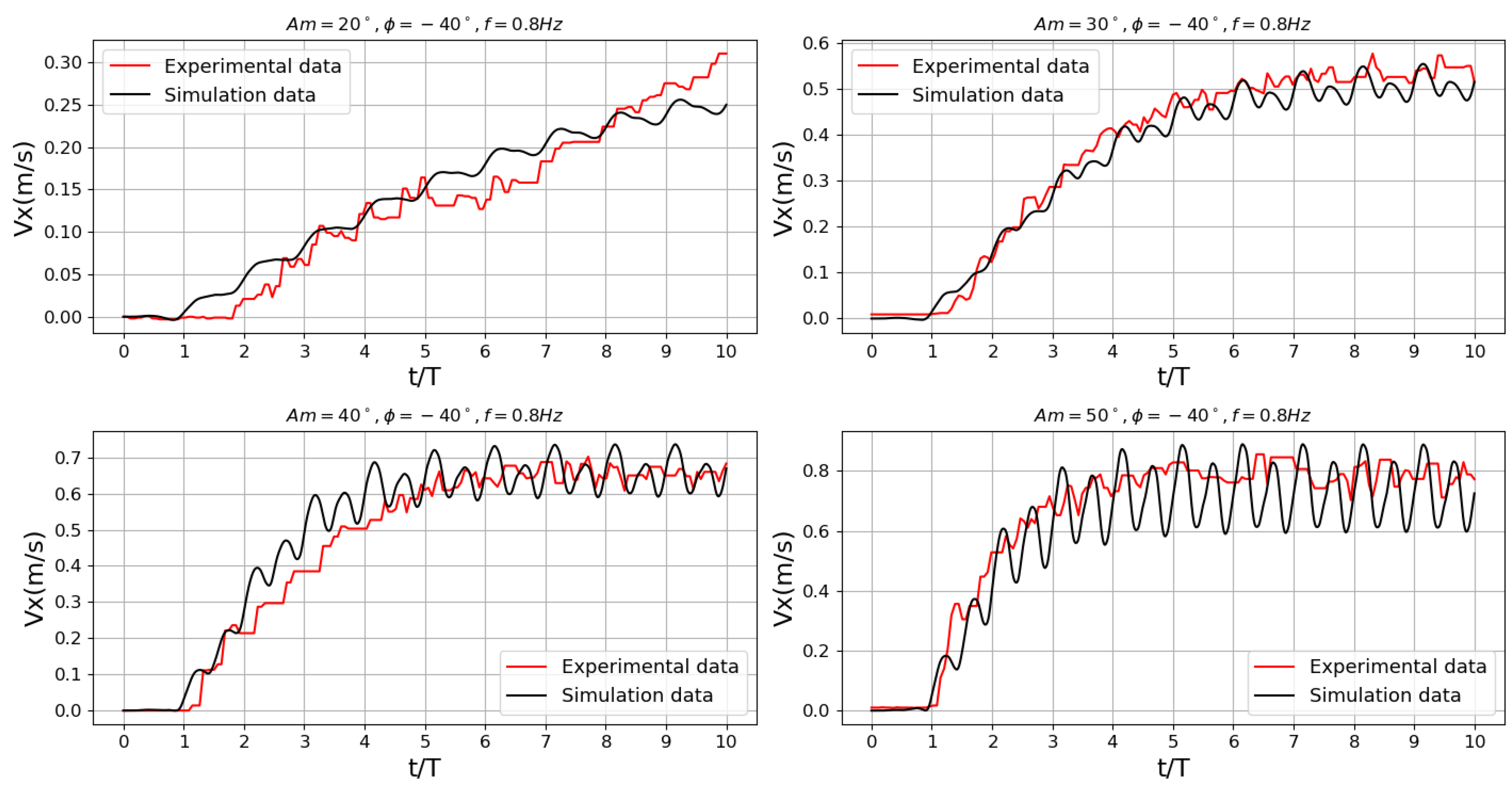
5.1. Verification of Wave Transmission

We initially validate the fundamental wave transmission motion of the MPF mode. Throughout the simulation, the motion of the body component in Figure 6 is excluded. The flexible fins flap up and down while fixed in the base, analogous to experiments involving a stationary fish fin in a water tank or wind tunnel experiments with a fixed wing.

In Figure 7, the entire flexible fins are divided into 30 different rod systems based on the previous modeling process. Over two motion cycles, the amplitude variations of rod systems $q_k^1$ (the tip of the fin chord) and $q_k^{30}$ (the end of the fin chord) are respectively represented in black and red. The fin is divided into three sections in the spanwise direction, and the amplitude variations of each section are extracted to quantify the spanwise wave transmission. It can be observed that in the three passive segments ($q_1$, $q_2$, $q_3$), a conspicuous phenomenon of phase lag is evident, serving to mimic the transmission of biomimetic chordwise waves. Simultaneously, when selectively extracting the spanwise amplitude at the trailing edge of the passive fins ($q_1^{30}$, $q_2^{30}$, $q_3^{30}$), a highly noticeable phase lag phenomenon is observable, corresponding to the spanwise wave transmission of the manta rays.

Figure 8 shows the disparity between the calculated average thrust and the experimental results in [6] with changing amplitudes $Am$ and phase differences $\varphi$ at various driving frequencies. In the left figure, maintaining a phase difference of ${30}^{\circ }$, the simulated average thrust under various flapping amplitudes closely aligns with the experimental one. As the flapping amplitude approaches ${40}^{\circ }$, the thrust differences between red lines and blue lines become apparent. The thrust difference reaches the maximum (about 1.8 N) at the amplitude $Am={40}^{\circ }$ and the frequency $f=0.51$ Hz. This discrepancy is attributed to the lack of accuracy in the Morison equation when describing large amplitude motions. In the right figure, maintaining an amplitude of ${30}^{\circ }$, we varied the phase difference from $-{30}^{\circ }$ to ${30}^{\circ }$. It can be observed that the calculated trend of average thrust matches the experimental results. The error is relatively small when the phase difference is positive. In conclusion, the two sets of experiments effectively validated the reliability of our flexible fins model.

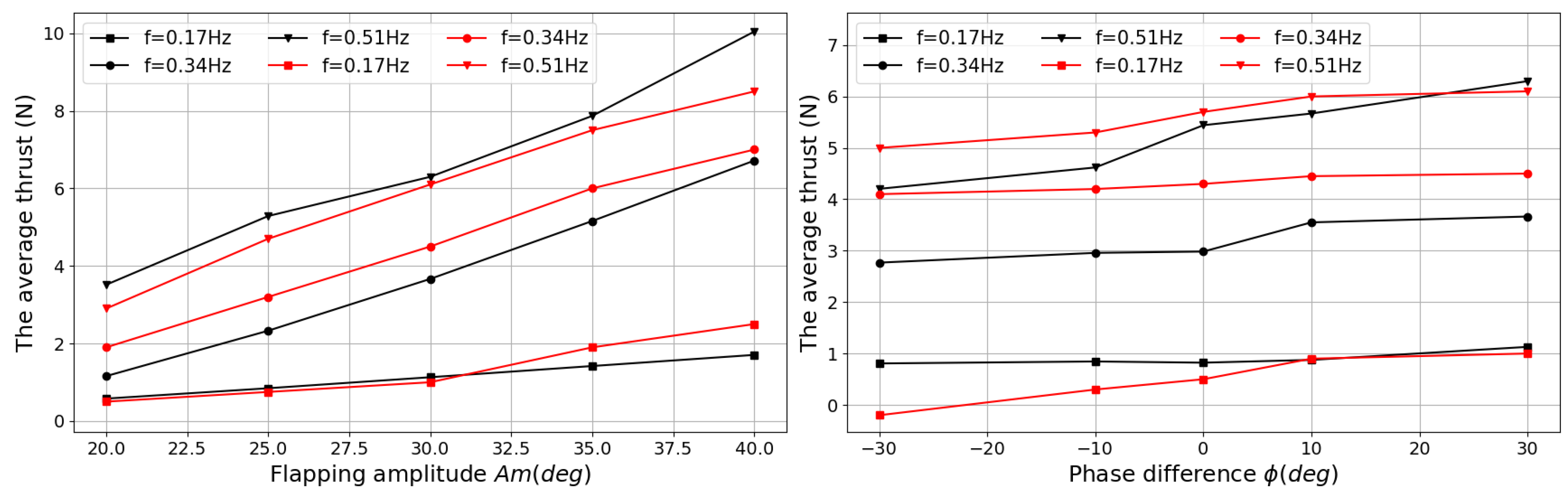
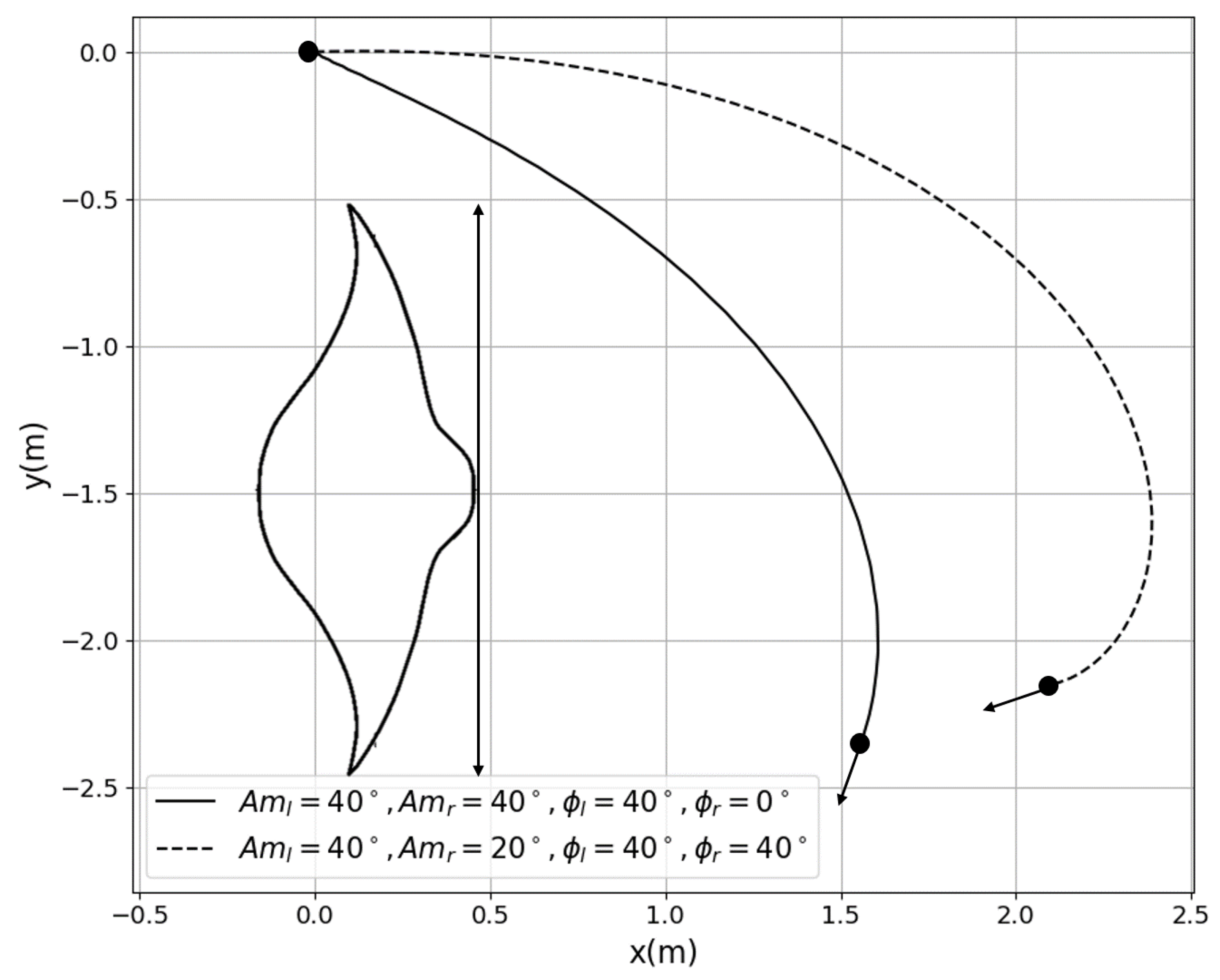
5.2. Simulation of Different Gaits

In Figure 9, we conducted a motion simulation of the entire robot during a straight gait, obtaining the time-varying velocity of the center of mass of the rigid body. The motion mode of MPF led to oscillations in forward velocity. keeping the input parameters constant, the velocity of the robot eventually converges and stabilizes. It can be observed that the simulated velocity, on average, closely aligns with the experimental results without significant differences. Simultaneously, as the flapping amplitude $Am$ increases, the oscillation amplitude of the robot’s forward velocity becomes larger. When the amplitude rises above ${40}^{\circ }$, the error becomes significant. Taking the amplitude $Am={50}^{\circ }$ as an example, the error of the average velocity reaches 0.07 m/s (average velocities are obtained between four and ten seconds). This discrepancy is attributed to the inaccuracy of Morison’s equation at large amplitude motions, as evidenced by the verification results for hydrodynamic forces in Figure 8. Nonetheless, the model proves accurate enough for a manta robot focused on dynamics and control.

In Figure 10, we present the motion trajectories obtained by adjusting various flapping amplitudes and phase differences on the left and right sides when maintaining a frequency of $0.8\mathrm{Hz}$. The asymmetry in the phase difference of the drive mechanisms on both sides of the pectoral fins and the inconsistency in the flapping amplitudes can both give rise to the turning gaits. The solid curve represents respectively motion parameter set $A{m}_l={40}^{\circ }$, $A{m}_r={40}^{\circ },{\varphi }_l={40}^{\circ },{\varphi }_r=0^{\circ }$ and the dotted curve represents $A{m}_l={40}^{\circ },A{m}_r={20}^{\circ },$ ${\varphi }_l={40}^{\circ }$, ${\varphi }_r={40}^{\circ }$.

Finally, Figure 11 shows the resultant wrench of two types of turning swimming. Comparing the primary moment $m_z$, it can be observed that the turning mode, which involves altering the phase difference, ${\varphi }_l$ and ${\varphi }_r$, exhibits a higher rotational acceleration during the initial stages of motion. On the other hand, the turning mode associated with amplitude variations, $A{m}_l$ and $A{m}_r$, can consistently generate a stable driving moment, making it suitable for cruising swimming with circular trajectories. The relationship between hydrodynamic performance and the above factors is a complicated question and warrants further detailed research to explore improved swimming gaits.

6. Conclusions

In this paper, we have presented a multibody dynamics model dedicated to the rigid-flexible coupling dynamics of underwater robots with a tree-like structure having both active and passive parts. Moreover, the hydrodynamics of the robot was calculated by the Morison equation, and the passive deformation of the flexible fins was taken into account by a PRB model. Based on the NEDA, the proposed approach can solve the rigid-flexible coupling dynamic problems together with a sequential coupling technology. As illustrated in Section 5, in the case of the manta robot, the given solution is computationally efficient. In particular, we have been able to numerically recover the characteristic hydrodynamic forces of the robotic manta during different motion gaits.

The ongoing and future work will focus on conducting parameter identification using a substantial dataset of experimental data to correct the model parameters and enable 3D path planning control. From the modeling point of view, the framework will be further developed to account for additional deformation DOFs and various constraints. The modeling approach will also be further extended to include more aquatic organisms.

References

1. Dharmdas, A.; Patil, A.Y.; Baig, A.; Hosmani, O.Z.; Mathad, S.N.; Patil, M.B.; Kumar, R.; Kotturshettar, B.B.; Fattah, I.M.R. An Experimental and Simulation Study of the Active Camber Morphing Concept on Airfoils Using Bio-Inspired Structures. Biomimetics 2023, 8, 251. [Google Scholar] [CrossRef] [PubMed]
2. Patil, A.Y.; Hegde, C.; Savanur, G.; Kanakmood, S.M.; Contractor, A.M.; Shirashyad, V.B.; Chivate, R.M.; Kotturshettar, B.B.; Mathad, S.N.; Patil, M.B.; et al. Biomimicking Nature-Inspired Design Structures—An Experimental and Simulation Approach Using Additive Manufacturing. Biomimetics 2022, 7, 186. [Google Scholar] [CrossRef] [PubMed]
3. Cui, Z.; Yang, Z.; Shen, L.; Jiang, H. Complex modal analysis of the movements of swimming fish propelled by body and/or caudal fin. Wave Motion 2018, 78, 83–97. [Google Scholar] [CrossRef]
4. Kato, N. Median and paired fin controllers for biomimetic marine vehicles. Appl. Mech. Rev. 2005, 58, 238–252. [Google Scholar] [CrossRef]
5. Dewar, H.; Mous, P.; Domeier, M.; Muljadi, A.; Pet, J.; Whitty, J. Movements and site fidelity of the giant manta ray, Manta birostris, in the Komodo Marine Park, Indonesia. Mar. Biol. 2008, 155, 121–133. [Google Scholar] [CrossRef]
6. Xing, C.; Cao, Y.; Cao, Y.; Pan, G.; Huang, Q. Asymmetrical oscillating morphology hydrodynamic performance of a novel bionic pectoral fin. J. Mar. Sci. Eng. 2022, 10, 289. [Google Scholar] [CrossRef]
7. Belkhiri, A.; Porez, M.; Boyer, F. A hybrid dynamic model of an insect-like mav with soft wings. In Proceedings of the 2012 IEEE International Conference on Robotics and Biomimetics (ROBIO), Guangzhou, China, 11–14 December 2012; IEEE: Piscataway, NJ, USA, 2012; pp. 108–115. [Google Scholar]
8. Porez, M.; Boyer, F.; Belkhiri, A. A hybrid dynamic model for bio-inspired soft robots—Application to a flapping-wing micro air vehicle. In Proceedings of the 2014 IEEE International Conference on Robotics and Automation (ICRA), Hong Kong, China, 31 May–7 June 2014; IEEE: Piscataway, NJ, USA, 2014; pp. 3556–3563. [Google Scholar]
9. Boyer, F.; Porez, M. Multibody system dynamics for bio-inspired locomotion: From geometric structures to computational aspects. Bioinspir. Biomim. 2015, 10, 025007. [Google Scholar] [CrossRef] [PubMed]
10. Khalil, W. Dynamic modeling of robots using recursive newton-euler techniques. In Proceedings of the ICINCO 2010, 7th International Conference on Informatics in Control, Automation and Robotics, Madeira, Portugal, 15–18 June 2010. [Google Scholar]
11. Meng, Y.; Wu, Z.; Dong, H.; Wang, J.; Yu, J. Toward a Novel Robotic Manta With Unique Pectoral Fins. IEEE Trans. Syst. Man Cybern. Syst. 2020, 52, 1663–1673. [Google Scholar] [CrossRef]
12. Corke, P.; Trevelyan, J.; Mason, R.; Burdick, J. Construction and modelling of a carangiform robotic fish. In Experimental Robotics VI, Proceedings of the 6th International Symposium on Experimental Robotics; Sydney, Australia, 26–28 March 1999, Springer: Berlin/Heidelberg, Germany, 2000; pp. 235–242. [Google Scholar]
13. Yu, J.; Yuan, J.; Wu, Z.; Tan, M. Data-driven dynamic modeling for a swimming robotic fish. IEEE Trans. Ind. Electron. 2016, 63, 5632–5640. [Google Scholar] [CrossRef]
14. Khan, A.; Wang, X.; Li, Z.; Wang, L.; Elahi, A.; Imran, M. Analytical and Numerical Study of Underwater Tether Cable Dynamics for Seabed Walking Robots Using Quasi-Static Approximation. J. Mar. Sci. Eng. 2023, 11, 1539. [Google Scholar] [CrossRef]
15. Lighthill, M. Hydromechanics of aquatic animal propulsion. Annu. Rev. Fluid Mech. 1969, 1, 413–446. [Google Scholar] [CrossRef]
16. Lighthill, M.J. Large-amplitude elongated-body theory of fish locomotion. Proc. R. Soc. Lond. Ser. B Biol. Sci. 1971, 179, 125–138. [Google Scholar]
17. Porez, M.; Boyer, F.; Ijspeert, A.J. Improved Lighthill fish swimming model for bio-inspired robots: Modeling, computational aspects and experimental comparisons. Int. J. Robot. Res. 2014, 33, 1322–1341. [Google Scholar] [CrossRef]
18. Liu, Q.; Chen, H.; Wang, Z.; He, Q.; Chen, L.; Li, W.; Li, R.; Cui, W. A Manta Ray Robot with Soft Material Based Flapping Wing. J. Mar. Sci. Eng. 2022, 10, 962. [Google Scholar] [CrossRef]
19. Design and implementation of multi-level linkage mechanism bionic pectoral fin for manta ray robot. Ocean Eng. 2023, 284, 115152. [CrossRef]
20. Liljebäck, P.; Pettersen, K.Y.; Stavdahl, Ø.; Gravdahl, J.T. Snake Robots: Modelling, Mechatronics, and Control; Springer: Berlin/Heidelberg, Germany, 2013. [Google Scholar]
21. Armanini, C.; Boyer, F.; Mathew, A.T.; Duriez, C.; Renda, F. Soft robots modeling: A structured overview. IEEE Trans. Robot. 2023, 39, 1728–1748. [Google Scholar] [CrossRef]
22. Huang, W.; Liu, M.; Hsia, K.J. A discrete model for the geometrically nonlinear mechanics of hard-magnetic slender structures. Extrem. Mech. Lett. 2023, 59, 101977. [Google Scholar] [CrossRef]
23. Li, Q.; Chen, T.; Chen, Y.; Wang, Z. An underwater bionic crab soft robot with multidirectional controllable motion ability. Ocean Eng. 2023, 278, 114412. [Google Scholar] [CrossRef]
24. Colbrook, M.J.; Townsend, A. Rigorous data-driven computation of spectral properties of Koopman operators for dynamical systems. Commun. Pure Appl. Math. 2024, 77, 221–283. [Google Scholar] [CrossRef]
25. Habibi, H.; Yang, C.; Godage, I.S.; Kang, R.; Walker, I.D.; Branson, D.T., III. A Lumped-Mass Model for Large Deformation Continuum Surfaces Actuated by Continuum Robotic Arms. J. Mech. Robot. 2019, 12, 011014. [Google Scholar] [CrossRef]
26. Troeung, C.; Liu, S.; Chen, C. Modelling of Tendon-Driven Continuum Robot Based on Constraint Analysis and Pseudo-Rigid Body Model. IEEE Robot. Autom. Lett. 2023, 8, 989–996. [Google Scholar] [CrossRef]
27. Naughton, N.; Sun, J.; Tekinalp, A.; Parthasarathy, T.; Chowdhary, G.; Gazzola, M. Elastica: A compliant mechanics environment for soft robotic control. IEEE Robot. Autom. Lett. 2021, 6, 3389–3396. [Google Scholar] [CrossRef]
28. Howell, L.L.; Midha, A.; Norton, T.W. Evaluation of equivalent spring stiffness for use in a pseudo-rigid-body model of large-deflection compliant mechanisms. J. Mech. Des. 1996, 118, 126–131. [Google Scholar] [CrossRef]
29. Day, R.E. Coupling Dynamics in Aircraft: A Historical Perspective; National Aeronautics and Space Administration, Office of Management, Scientific and Technical Information Program: Washington, DC, USA, 1997; Volume 532. [Google Scholar]
30. El-Hawary, F. The Ocean Engineering Handbook; CRC Press: Boca Raton, FL, USA, 2000. [Google Scholar]
31. Chenevier, J.; González, D.; Aguado, J.V.; Chinesta, F.; Cueto, E. Reduced-order modeling of soft robots. PLoS ONE 2018, 13, e0192052. [Google Scholar] [CrossRef]
32. Bao, P.; Shi, L.; Zhang, Z.; Guo, S. Kinematics Simulation Based on Fluent of a Bionic Manta ray Robot. In Proceedings of the 2021 IEEE International Conference on Unmanned Systems (ICUS), Beijing, China, 15–17 October 2021; pp. 249–254. [Google Scholar]
33. Jawed, M.; Novelia, A.; O’Reilly, O. A Primer on the Kinematics of Discrete Elastic Rods; SpringerBriefs in Applied Sciences and Technology; Springer International Publishing: Berlin/Heidelberg, Germany, 2018. [Google Scholar]
34. Xie, X.; Herault, J.; Lebastard, V.; Boyer, F. Recursive inverse dynamics of a swimming snake-like robot with a tree-like mechanical structure. In Proceedings of the 2023 IEEE International Conference on Advanced Robotics and Its Social Impacts (ARSO), Berlin, Germany, 5–7 June 2023; IEEE: Piscataway, NJ, USA, 2023; pp. 65–70. [Google Scholar]
35. Khalil, W.; Gallot, G.; Boyer, F. Dynamic modeling and simulation of a 3-D serial eel-like robot. IEEE Trans. Syst. Man, Cybern. Part C (Appl. Rev.) 2007, 37, 1259–1268. [Google Scholar] [CrossRef]
Figure 1. The schematic diagram of a fixed-basis multibody system (left) and a mobile multibody system (right).
Jmse 12 00292 g001
Figure 2. Schematic representation of the actuation mechanism (black left part) and the left pectoral fin’s passive pseudo-rigid body model (blue right part).
Jmse 12 00292 g002
Figure 3. The illustration of the tangent direction vectors  n  and the velocity  V c m  of the discrete flexible pectoral fins.
Jmse 12 00292 g003
Figure 4. Schematic representation of the connection between the robot body and one linkage of parallel PRB system of the (left) flexible fin with three DoF. The red and blue arrows represent respectively the linear and angular accelerations and the forces and torques. The black line represents the active link and the blue lines are the passive links.
Jmse 12 00292 g004
Figure 5. Pseudo rigid body assumption of a discrete rod: the discrete curvature at jth node.
Jmse 12 00292 g005
Figure 6. Flow chart of the Rigid-Flexible Coupling dynamic algorithm.
Jmse 12 00292 g006
Figure 7. Verification of the chordwise and spanwise wave transmission.
Jmse 12 00292 g007
Figure 8. Influences of different oscillation parameters on the average thrust. The left and right figures represent respectively the influences of the flapping amplitude  A m  and the phase different  ϕ . Black and red curves represent the data obtained respectively by numerical simulation and by experiments of the prototype.
Jmse 12 00292 g008
Figure 9. Comparison of the swimming speed between experimental and simulation data with the flapping parameters  A m = 40 ϕ = 40  and  f = 0.6  Hz.
Jmse 12 00292 g009
Figure 10. Comparison of two types of turning swimming with the fixed oscillation frequency  f = 0.8  Hz simulated during in 20 periods.
Jmse 12 00292 g010
Figure 11. Comparison of the resultant wrench of two types of turning swimming. The solid and dotted curves represent respectively motion parameter sets  ( A m l = 40 , A m r = 40 , ϕ l = 40 , ϕ r = 0 )  and  ( A m l = 40 , A m r = 20 , ϕ l = 40 , ϕ r = 40 ) .
Jmse 12 00292 g011