Circumferential Background Field Temperature Inversion Prediction and Correction Based on Ground-Based Microwave Remote Sensing Data

Abstract

Microwave radiometers are passive remote sensing devices that provide important observational data on the state of the oceanic and terrestrial atmosphere. Temperature retrieval accuracy is crucial for radiometer performance. However, inversions during strong convective weather or seasonal phenomena are short-lived and spatially limited, making it challenging for neural network algorithms trained on historical data to invert accurately, leading to significant errors. This paper proposes a long short-term memory (LSTM) network forecast correction model based on the temperature inversion phenomenon to resolve these large temperature inversion errors. The proposed model leverages the seasonal periodicity of atmospheric temperature profiles in historical data to form a circumferential background field, enabling the prediction of expected background profiles for the forecast day based on temporal and spatial continuity. The atmospheric profiles obtained using the radiometer retrieval are compensated with the forecast temperature inversion vector on the forecast day to obtain the final data. In this study, the accuracy of the forecast correction model was verified utilizing meteorological records for the Taizhou area from 2013 to 2017. Using a hierarchical backpropagation network based on the residual module for comparison, which had a forecast accuracy error of 0.0675 K, the error of our new model was reduced by 34% under the temperature inversion phenomenon. Meanwhile, error fluctuations were reduced by 33% compared with the residual network algorithm, improving the retrieval results’ stability in the temperature inversion state. Our results provide insights to improve radiometer remote sensing accuracy.

1. Introduction

Microwave radiometers are key in monitoring climatic scenarios, such as those on coastlines, and are important equipment for marine environment monitoring. Microwave radiometers are widely used for their all-weather passive remote sensing properties, where atmospheric radiation is measured and calibrated to produce brightness temperatures, which are then inverted by algorithms to obtain meteorological information such as temperature and humidity profiles [1]. A more accurate observation of atmospheric parameters is important to improve the performance of radiometer parameters. Two main methods exist to improve retrieval accuracy: physical and statistical. Neural networks use historical data to develop mathematical models based on statistical methods. The physical inverse method obtains atmospheric temperature profiles by solving the atmospheric transport equation. Westwater [1] introduced the root mean square method for analyzing vertical profiles of atmospheric parameters. Smith [2] developed a physical iterative technique that bypassed the need for historical–sounding data. The method uses a step-by-step approximation to efficiently estimate the temperature information of the vertical profiles of atmospheric parameters and establishes accurate data on the distribution of the vertical stratified structure of the atmosphere. Xiong [3] applied a one-dimensional (1D) variational approach to retrieve atmospheric parameters, achieving substantially improved results in high-altitude temperatures and humidity retrieval compared to the outcomes from the RPG microwave radiometer’s built-in algorithm. Yang [4] used the 1D variational method to retrieve temperature and water vapor metrics in clear-sky scenarios and discovered that the mean temperature error below 4 km was less than 0.2 K. Numerical methods can obtain high accuracy. However, they have disadvantages, including slow operation speed. With the development of computer hardware and software technologies, retrieval algorithms based on neural networks have become widely used. Churnside et al. [5] first applied neural networks to produce microwave radiometer retrievals. Valjarević et al. studied long-term monitoring of stratospheric clouds using high-optical imagery, satellite data, GIS, and RS. It explored cloud properties, types, and climate impacts, with new findings on water vapor. The research highlights the influence of these clouds on climate change [6]. Cimini et al. introduced a neural Network (NN) for radiometer retrieval, and its experimental results are similar to those obtained by the regularization method [7]. Most radiometer-based atmospheric profile retrievals started using backpropagation neural networks (BPNN) [8,9]. As these network types progressed, a variety of networks were developed. Luo et al. used four machine learning algorithms, namely, deep learning (DL), gradient boosting machine (GBM), extreme gradient boosting (XGBoost), and random forest (RF) for the retrieval of atmospheric contours and concluded that deep learning performed optimally among the four methods [10].

The deep learning model performed the most effectively in temperature retrievals with a root mean square error and correlation coefficient of 2.36 K and 0.98, respectively. Pathak et al. developed an inverse algorithm to analyze the vertical structure of temperature and specific humidity using feed-forward neural networks, its results effectively improve the resolution of atmospheric profiles above 2000 m [11]. Renju et al. [12] observed the tropical waters of the Indian Ocean based on DL, and the temperature error converged at 1.4 K. Both physical and neural network methods have been extensively developed in the field of radiometer retrieval. However, relatively little modeling of the two conjointly using the fusion approach has occurred. Merging the two methods using background fields combines the accuracy of physical retrieval with the speed of neural networks. In 1950, Charney et al. [13] introduced a method that leveraged spatial interpolation to convert low-resolution datasets into high-resolution fixed-point data backgrounds. Wilby et al. developed a Statistical Downscaling Model (SDSM) to examine a weather generator and conduct linear regression, confirming its precision through testing. Precision was confirmed by testing [14]. Sun L et al. suggested the use of kriging interpolation and discrete smooth interpolation (DSI) and found that kriging interpolation outperformed DSI in terms of accuracy [15]. Therefore, choosing a suitable background field for examining the conformity between physical methods and neural networks is important. The background fields reflect diverse regions and climates [16]. The background fields of different climatic seasons can flexibly respond to the daily meteorological conditions at the observation site. Temperature changes caused by different climatic phenomena correspond to the true fluctuations of the temperature profiles observed by the radiometer. Generally, greater seasonal weather changes occurred on consecutive observation days with strong profile fluctuations, making it difficult to perform an accurate and efficient retrieval using only one retrieval method.

Fluctuations in temperature profiles, partially attributed to seasonal climatic factors, are investigated in this paper. Zhao et al. proposed the use of a highly hierarchical back-propagation (BP) network for the inversion of brightness temperatures, which improves the retrieval efficiency by a factor of ten, while the error is comparable to that of the initial algorithm (NN network) [17]. On this basis, we also proposed a retrieval model based on a residual network in the related paper of the prelude study, which improves the accuracy of water vapor density observation in response to the problems of data collapse of the BP algorithm. Compared with the traditional radiometer retrieval network, the temperature accuracy of the residual network-based retrieval model is improved by 20% [16]. In this paper, a deeper optimization based on the residual network algorithm model is presented.

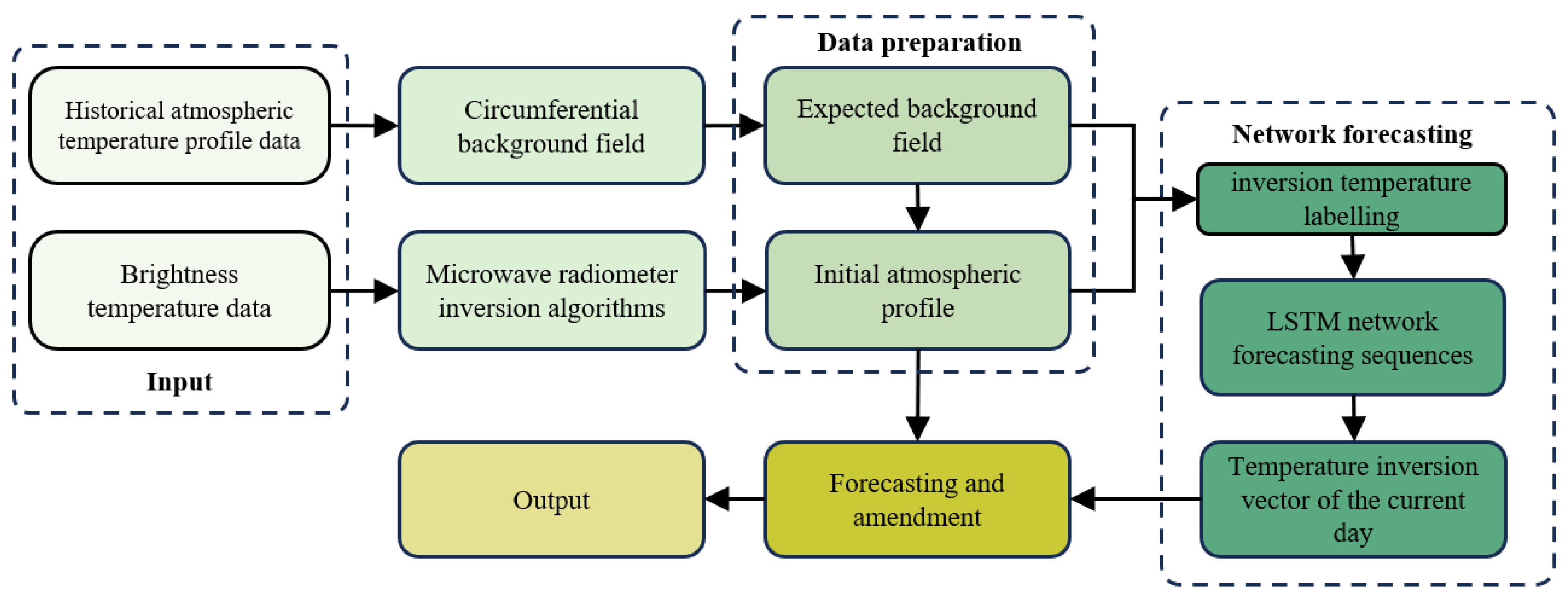
This study proposes a forecast correction model for annular background fields based on a residual retrieval network; this is a mathematical model that uses the climate distribution to generate the background field based on historical data, outputs the desired profile for the day, then the temperature inversion forecasting module generates a temperature inversion label for the day and produces a temperature inversion vector from the forecast. The brightness temperature data collected by the radiometer receiver were inverted to obtain the initial atmospheric profile; this was corrected by or combined with the temperature inversion vector of the current day to obtain the final data. To verify the solution to this problem, three experiments were designed using the radiosonde sounding data from 2013 to 2017 at Taizhou Weather Station as the true values and the brightness temperature observed by the radiometer for the same period as the measurement data. The three experiments verified the optimal parameters of the LSTM forecast network, the reliability of the background field expectation profile, and forecast correction. The experimental results were then analyzed.

The remainder of this paper is organized as follows: In Section 2, we designed a circumferential background field based on climate regression theory and then generated temperature inversion labels based on the circumferential background field. Section 3 discusses the LSTM forecast network, conducts parameter screening experiments, and analyzes the results. In Section 4, two validation experiments, namely, for the background field expectation profile and forecast correction, are presented, and the conclusions are analyzed. Finally, Section 5 presents the conclusions.

2. Methodology

The algorithm for forecasting and correcting the retrievals in the annular background field is a correction algorithm for the meteorological conditions of inversions. The temperature inversion forecasting module generates a temperature inversion label for the day and produces a temperature inversion vector from the forecast. The brightness temperature data collected by the radiometer receiver were inverted to obtain the initial atmospheric profile; this was compensated by the temperature inversion vector of the current day to obtain the final data. The general framework of this paper is shown in Figure 1.

This section presents the mathematical model in two parts. The first part is the generation of a background field based on cyclic variations in climate using the circumferential background field formed by historical radiosonde sounding data, and the desired background field profile on the forecast day is based on the spatial and temporal continuity of atmospheric parameters. The second part is the temperature inversion calibration. This section first introduces the inversion phenomenon and its causes. Then, an inversion labeling method is proposed based on the expected background field profiles derived in the first part.

2.1. Expected Background Field Profile Model

The data used in this study to prepare the background field are atmospheric profile data from Taizhou City, Zhejiang Province, China, and they were collected over five years at sampling intervals of 12 h. Taizhou City is located in 120°17′–121°56′ E and 28°01′–29°20′ N, which is a coastal city, close to a river estuary. The data are from radiosondes released by weather stations in the area, 121°34′ E and 28°47′ N; the observatory site is located in the waterfront area at that latitude and longitude. At the same time, microwave radiometers are measuring in the area where the weather station is located. The radiometer model used in the experiment is MP3000A (Microwave Radiometer, Boulder, CO, USA), which receives electrical signals from the atmosphere and converts them into a bright temperature signal, which is then inverted into an atmospheric temperature profile. The improved inversion algorithm used in this microwave radiometer is a residual network with a height resolution of 100 m measuring a maximum height of 10 km [17]. This region is a central subtropical monsoonal area with four distinct seasons. Taizhou city is mainly influenced by the East Asian monsoon circulation. In summer, the prevailing southeast monsoon from the ocean brings moist airflow and abundant precipitation; in winter, it is influenced by the northerly wind from the inland, which makes the airflow relatively dry and the precipitation less. As Taizhou is located in the coastal area, the frequent typhoon activities during the summer and autumn seasons each year may have a significant impact on the atmospheric circulation in the Taizhou area, bringing strong winds, heavy rain, and other weather phenomena.

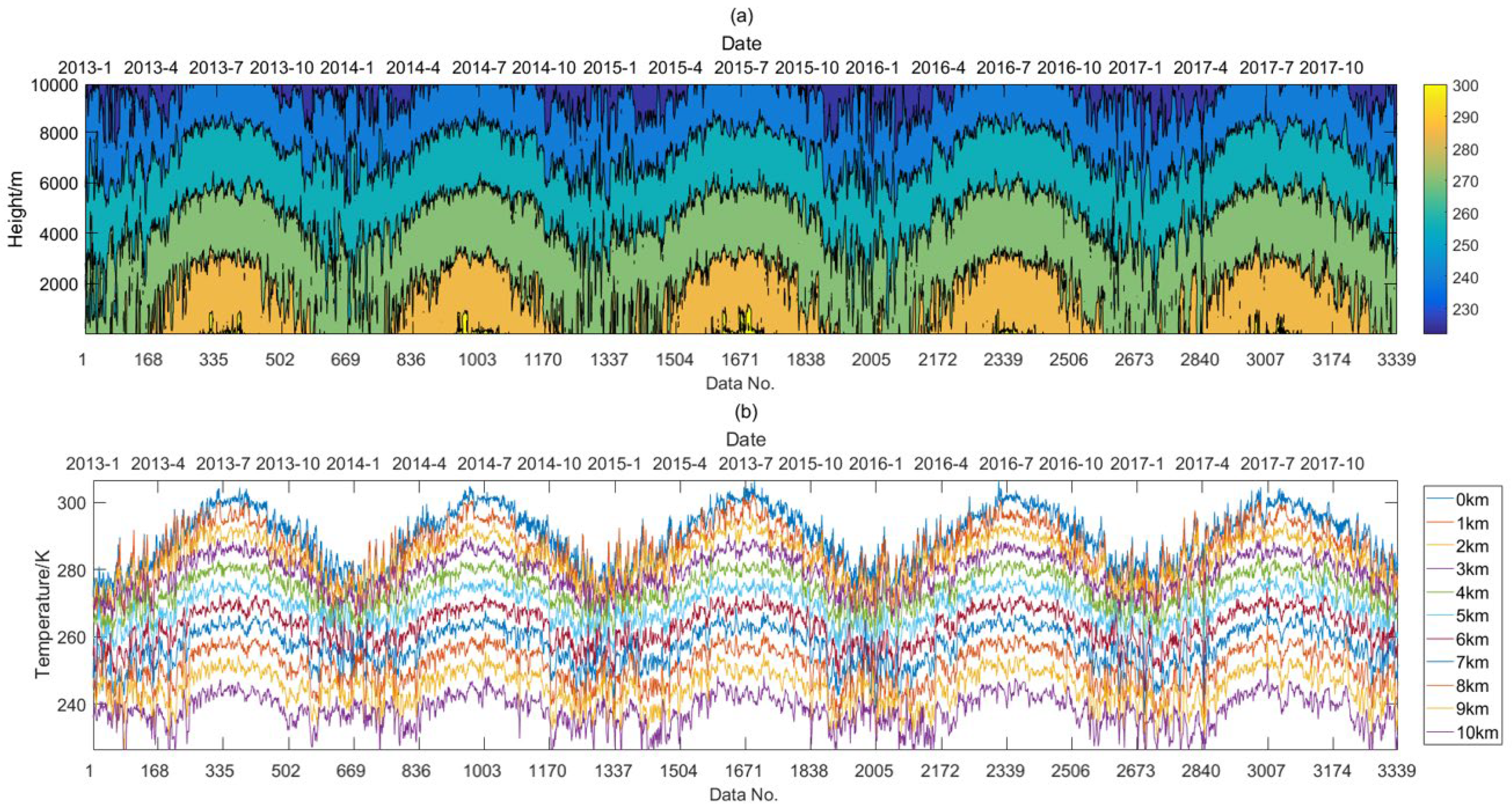
Due to the monsoon’s influence, the Taizhou atmospheric temperature profile changed, as shown in Figure 1.

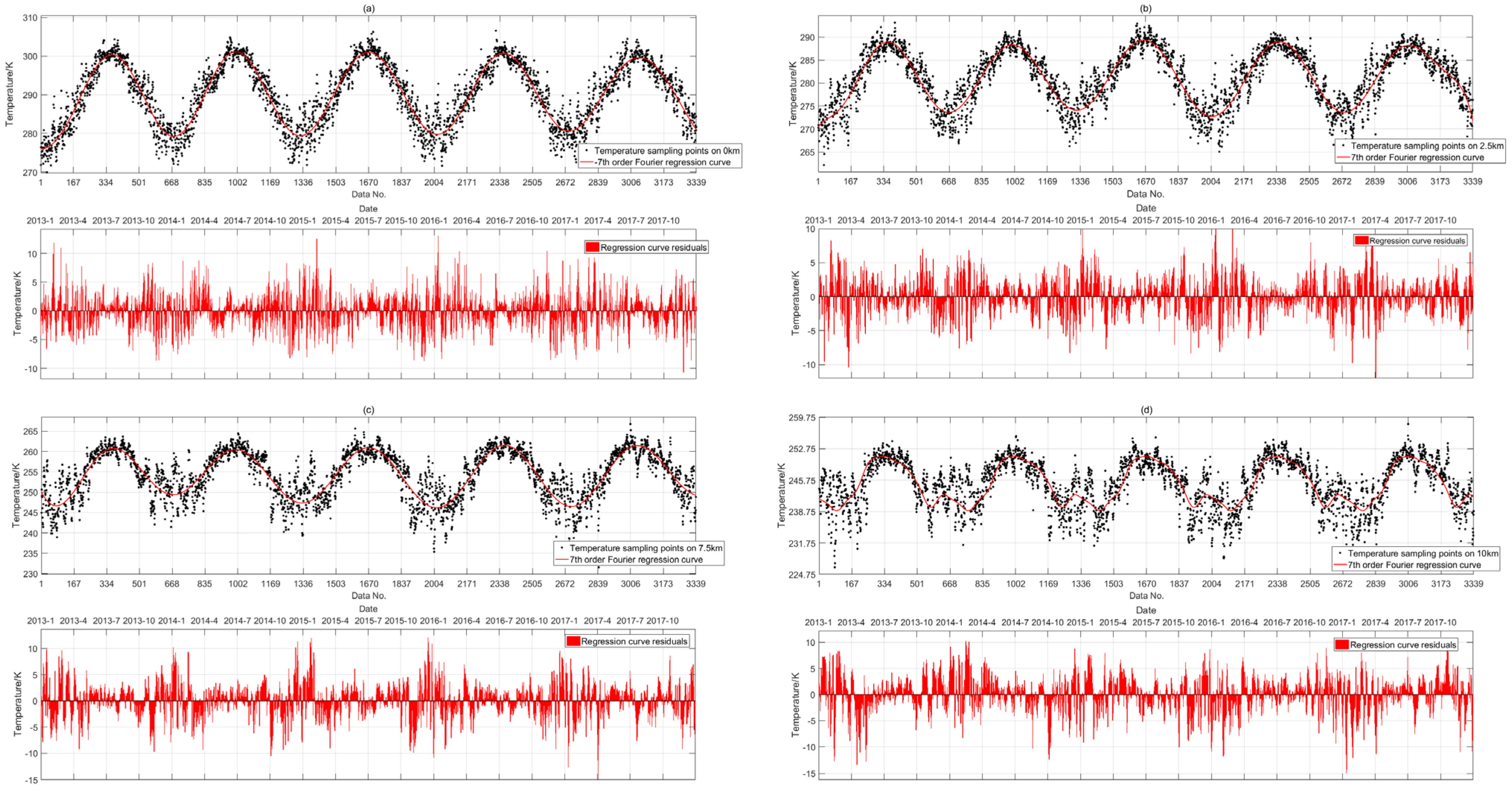
Figure 2 shows that the atmospheric temperature in Taizhou is cyclic for the isothermal layer and the temperature change of the profile lines within the observed data, and the minimum period of this cycle is in units of one year [18]. In a single cyclic cycle, isothermal and isopause temperatures oscillate significantly in fall and winter and level off in spring and summer. These two trends exhibit the same conditions in all cycles within the data range. To further regress the cyclic temperature changes in the region, a periodic function regression was used to fit the temperatures at multiple heights, and the results shown in Figure 3 were obtained.

Figure 3 shows that the temperature variations in each altitude stratum over five years can be approximated and regressed using a seventh-order Fourier fit [19,20,21,22,23], where the temperatures in the middle and bottom of the troposphere have only one peak in a temperature fluctuation cycle. However, as the altitude is increased to the layer where the top of the troposphere meets the stratosphere, two highly inconsistent peaks appear. However, these fluctuations can be regressed by a same-order (7th order) Fourier regression within a certain error range. Based on these results, we draw the following three conclusions:

• Law 1: Climate change is continuous in the localized area near the meteorological observation site in Taizhou and can be regarded as a change obeying a certain distribution.
• Law 2: Climate change in each quarter follows a fixed climate distribution.
• Law 3: The expected profiles of the mean temperature close to the current month are $S_1, S_2, S_3,$ and $S_4$ near the center date of each quarter.

Based on these three conclusions, the background field was established.

Figure 4 is based on data from Taizhou, China, which consists of atmospheric profiles $S_{(t,h)}$ for $T_0$ days. $T_0$ is taken as 365 or 366 when considering a leap year. $S_{(t,h)}$ represents the temperature ensemble of the atmospheric temperature profile for different dates $t$ at all heights $h$. The entire annular background field is divided into four parts, each with $T_0/4d$ (rounded down), where the seasonal cut-off dates are $\alpha ,\beta ,\gamma , \mathrm{a}\mathrm{n}\mathrm{d} \delta$. Seasonal regulations for subtropical and temperate monsoon climates in the Northern Hemisphere are more fixed, generally meaning that winter includes December through February, spring includes March through May, summer includes June through August, and fall includes September through November.

Spring is between α and β, summer is between β and γ, fall is between γ and δ, and winter is between δ and α. The temperature profiles of the entire annular background field were divided into four parts, each with $T_0/4d$ (rounded down), where $tgt$ denotes an arbitrarily selected target background field.

According to laws 1 and 2, the climate distribution obeys the $F_{season}$, hereafter referred to as $F_{se}$; $F_{se}$ denotes the statistical climate regression distribution for the season. In profile region $D$ at different times, we have the following:

$$D\left(S_{\left(t_{\alpha ,}h\right)},S_{\left(t_{\beta ,}h\right)}\right)~F_{spr}$$

(1)

Here, $D\left(S_{\left(t_{\alpha ,}h\right)}, S_{\left(t_{\beta ,}h\right)}\right)$ denotes the region that obeys the spring profile influence distribution $F_{spr}$, where $D\left(S_{\left(t_{\alpha ,}h\right)}, S_{\left(t_{\beta ,}h\right)}\right)$ denotes the spring background field profile region from α to β. Similarly, they are expressed as follows:

$$D\left(S_{\left(t_{\beta ,}h\right)}, S_{\left(t_{\gamma ,}h\right)}\right)~F_{sum}, D\left(S_{\left(t_{\gamma ,}h\right)},S_{\left(t_{\delta ,}h\right)}\right)~F_{aut}, D\left(S_{\left(t_{\delta ,}h\right)},S_{\left(t_{\alpha ,}h\right)}\right)~F_{win}$$

(2)

where $F_{sum},F_{aut}, \mathrm{a}\mathrm{n}\mathrm{d} F_{win}$ denote the profile influence distribution in summer, fall, and winter, respectively; and $D\left(S_{\left(t_{\beta ,}h\right)},S_{\left(t_{\gamma ,}h\right)}\right), D\left(S_{\left(t_{\gamma ,}h\right)},S_{\left(t_{\delta ,}h\right)}\right)$, and $D\left(S_{\left(t_{\gamma ,}h\right)},S_{\left(t_{\delta ,}h\right)}\right)$ denote the background field profile regions in summer, fall, and winter, respectively.

According to Law 3, for any background field profile, the temperature is affected by the current quarter and the quarter with the closest time distance to the current date. In $S_1,S_2,S_3, \mathrm{a}\mathrm{n}\mathrm{d} S_4,$ the date is in the center of the season, and the expected background field profile near the average temperature is only affected by the season’s temperature. Therefore, the desired background field $S_1$ is as follows:

$$E\left[{S_1}_{\left(t_{1,}h\right)}\right]={\int }_{\beta }^{\alpha }{S}_{\left(t,h\right)}\times F_{spr}\left\{D\left(S_{\left(t_{\alpha ,}h\right)},S_{\left(t_{\beta ,}h\right)}\right)\right\}dt$$

(3)

where $E$ denotes the expected value and $t_1$ denotes the date number where $S_1$ is located. Moreover, $E\left[{S_1}_{\left(t_{1,}h\right)}\right]$ denotes the desired background field at $S_1$. Similarly:

$$\begin{gathered} E\left[{S_2}_{\left(t_{2,}h\right)}\right]={\int }_{\gamma }^{\beta }{S}_{(t,h)}\times F_{sum}\left\{D\left(S_{\left(t_{\beta ,}h\right)},S_{\left(t_{\gamma ,}h\right)}\right)\right\}dt \\ E\left[{S_3}_{\left(t_{3,}h\right)}\right]={\int }_{\delta }^{\gamma }{S}_{(t,h)}\times F_{aut}\left\{D\left(S_{\left(t_{\gamma ,}h\right)},S_{\left(t_{\delta ,}h\right)}\right)\right\}dt \\ E\left[{S_4}_{\left(t_{4,}h\right)}\right]={\int }_{\alpha }^{\delta }{S}_{\left(t,h\right)}\times F_{win}\left\{D\left(S_{\left(t_{\delta ,}h\right)},S_{\left(t_{\alpha ,}h\right)}\right)\right\}dt \end{gathered}$$

(4)

Here, the desired background fields at $S_2,S_3,{ \mathrm{a}\mathrm{n}\mathrm{d} S}_4$ are indicated. The four background fields are referred to as the median background fields $S_m$.

$$S_m=\left\{S_1,S_2,S_3,S_4\right\}$$

(5)

Then, if the profile is located outside the four points, it is affected by the season closest to it; therefore, for the atmospheric profile at any time $t_0$, the desired background field profile is as follows:

$$E\left[{S_0}_{\left(t_0,h\right)}\right]=\mathsf{\eta }{\int }_{t_0}^{t_b}{S}_{\left(t,h\right)}\times F_{{se}_1}\left\{D\left(S_{\left(t_{a,}h\right)},S_{\left(t_{0,}h\right)}\right)\right\}dt+\left(1-\mathsf{\eta }\right){\int }_{t_0}^{t_a}{S}_{\left(t,h\right)}\times F_{{se}_2}\left\{D\left(S_{\left(t_{0,}h\right)},S_{\left(t_{b,}h\right)}\right)\right\}dt$$

(6)

In this equation,

$$\mathsf{\eta }={\displaystyle \frac{t_b-t_0}{0.25T}}$$

(7)

$t_a {\mathrm{a}\mathrm{n}\mathrm{d} t}_b$ denote the number of the two dates in the nearest median background field $S_m$ at profile $S_0$ ($t_b$ is located in the same season as $S_0$); $F_{{se}_1}$ denotes the seasonal distribution of profile $F_{{se}_1}$; $F_{{se}_2}$ denotes the distribution of profile impacts in the quarter that $S_0$ is located away from; and η denotes the seasonal impact share. Considering $S_{tgt}$ as an example and substituting Equations (1)–(4) and (7) into Equation (6), the expected background field profile is $E\left[{S_{tgt}}_{(t_{tgt},h)}\right]$ at $S_{tgt}$.

$$E\left[{S_{tgt}}_{\left(t_{tgt},h\right)}\right]={\displaystyle \frac{t_1-tgt}{0.25{\mathrm{T}}_0}}\times {\int }_{tgt}^{t_4}{S}_{\left(t,h\right)}\times F_{win}\left\{D\left(S_{\left(t_{\delta ,}h\right)},S_{\left(t_{\alpha ,}h\right)}\right)\right\}dt+{\displaystyle \frac{{tgt-t}_4}{0.25{\mathrm{T}}_0}}\times {\int }_{tgt}^{t_1}{S}_{\left(t,h\right)}\times F_{spr}\left\{D\left(S_{\left(t_{\alpha ,}h\right)},S_{\left(t_{\beta ,}h\right)}\right)\right\}dt$$

(8)

In this paper, the distribution of the background field influence is reported to use a uniform distribution. Then, the four median background fields are as follows:

$$\begin{gathered} E\left[{S_1}_{\left(t_{1,}h\right)}\right]=\sum _{\beta }^{\alpha }{S}_{\left(t,h\right)}/\sum _{\beta }^{\alpha }t \\ E\left[{S_2}_{\left(t_{2,}h\right)}\right]=\sum _{\gamma }^{\beta }{S}_{\left(t,h\right)}/\sum _{\gamma }^{\beta }t \\ E\left[{S_3}_{\left(t_{3,}h\right)}\right]=\sum _{\delta }^{\gamma }{S}_{(t,h)}/\sum _{\delta }^{\gamma }t \\ E\left[{S_4}_{\left(t_{4,}h\right)}\right]=\sum _{\alpha }^{\delta }{S}_{(t,h)}/\sum _{\alpha }^{\delta }t \end{gathered}$$

(9)

Then, the desired background field at $S_{tgt}$ can be expressed as follows:

$$E\left[{S_{tgt}}_{\left(t_{tgt},h\right)}\right]={\displaystyle \frac{\left|t_1-tgt\right|}{0.25{\mathrm{T}}_0}}\times \sum _{t_1}^{t_{tgt}}{S}_{\left(t,h\right)}/\sum _{t_1}^{t_{tgt}}t+{\displaystyle \frac{\left|{tgt-t}_4\right|}{0.25{\mathrm{T}}_0}}\sum _{t_{tgt}}^{t_4}{S}_{\left(t,h\right)}/\sum _{t_{tgt}}^{t_4}t$$

(10)

2.2. Temperature Inversion Labeling Model

Under normal circumstances, with the increase in altitude, the change in atmospheric temperature conforms to the law of a 0.6 K decrease for every 100 m of elevation, i.e., the mean altitudinal temperature gradient is −6 °C/km. However, because of the influence of some special weather conditions, the troposphere temperature will increase with an increase in altitude. In contrast, the atmospheric temperature, or the rate of change in atmospheric temperature, decrease is lower than that of the current altitude temperature change. This phenomenon occurs when temperature profiles contain inversions.

Based on the inversion causes, they can be categorized into the following six types:

• Radiative inversion. On cloudless nights, the loss of solar radiation causes a rapid decrease in near-surface temperatures. Meanwhile, less cooling occurs at high altitudes, resulting in an inversion.
• Advection inversion. When cold and warm air layers meet, the lower layer of the warm airflow is more affected by the influence of cold air; thus, the cooling rate is higher, and the upper layer of the warm airflow is slower. This results in the airflow meeting the height of the warmer and colder counter-temperature phenomenon. Moreover, this often occurs in the spring, fall, and winter seasons when the climate is volatile.
• Terrain inversion. This mainly occurs in basin areas because of the topography. The mountain slopes cool rapidly, the cold air on the mountain slopes gradually sinks to the bottom, and the bottom of the warm air exerts upward pressure, which leads to the occurrence of the temperature inversion phenomenon.
• Subsidence inversion. It is a phenomenon in which air temperature increases rather than decreases with altitude due to adiabatic warming of the airflow as it sinks. Subsidence inversion occurs mostly at high altitudes in high-pressure control areas, where vertical air convection is impeded.
• Turbulent temperature inversion. A variety of turbulence mixing, which leads to an air rise or fall phenomenon, will lead to the air temperature maintaining the normal top cold and bottom hot law. However, the weakening turbulence effect will lead to the emergence of the temperature inversion phenomenon.
• Cloud inversion. For observation of airspace with thick clouds in the troposphere, a temperature inversion phenomenon occurs because of the uneven reception of solar thermal radiation on the upper and lower surfaces of the clouds.

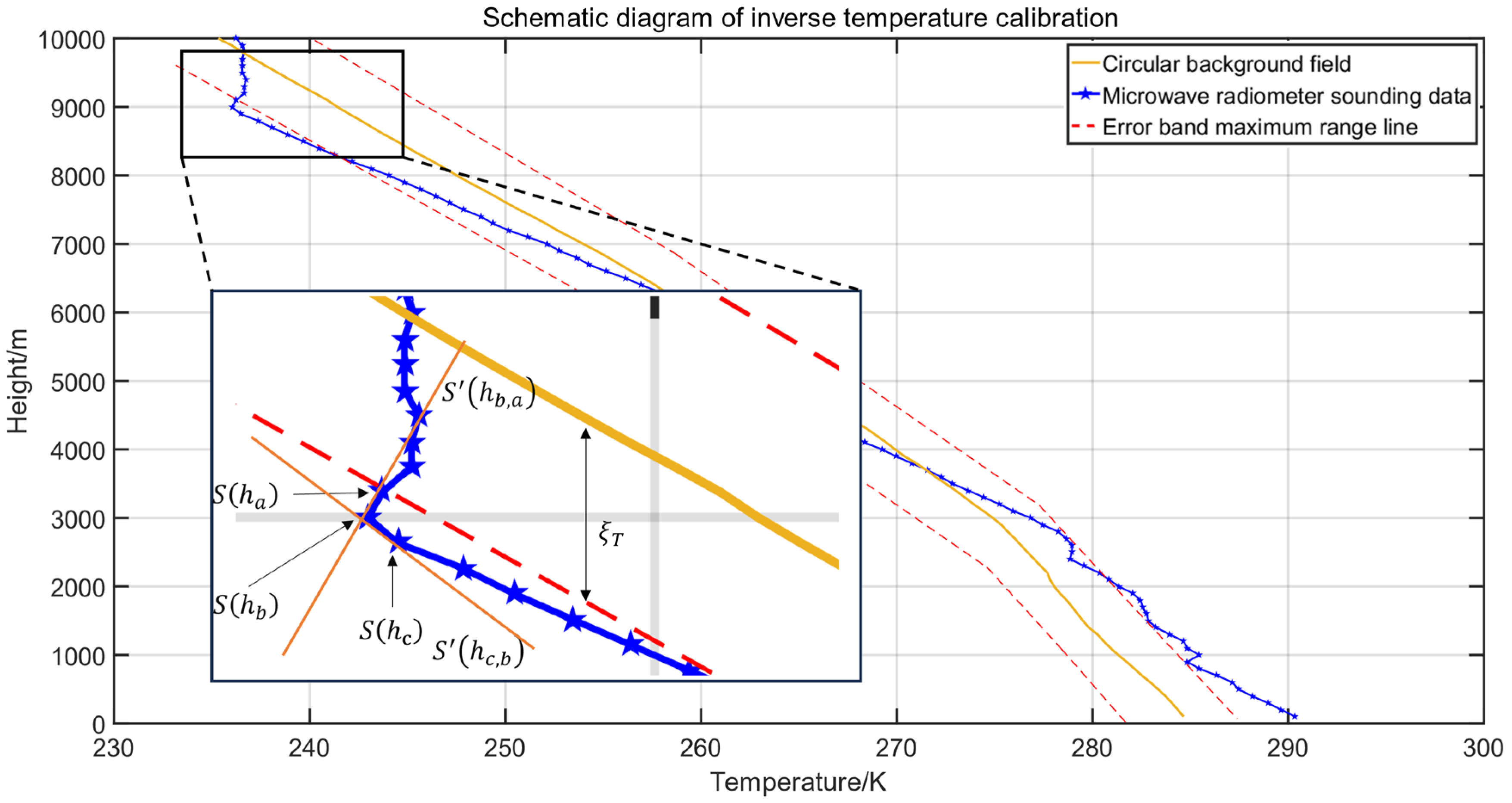
Given that the atmospheric profile is obtained by the radiometer or sounding balloon with an equal height scanning interval $h_f$, the profile is not continuous. Moreover, temperature inversion peaks will occur, and points with a height increase and a temperature change rate of 0 may not appear in the existing sampling points. To address this, the temperature inversion labeling method was used to calibrate the temperature inversion process.

The model for the temperature inversion calibration is schematically shown in Figure 5.

As illustrated in Figure 5, for any date $t$, a temperature inversion profile exists, and it presents heights from high to low neighboring sampling points a, b, and c, and then b to a sampling point between the rate of change of temperature $S^{\prime }\left(h_{b,a}\right)$, which can be described as follows:

$$S^{\prime }\left(h_{b,a}\right)={\displaystyle \frac{S\left(h_b\right)-S\left(h_a\right)}{h_b-h_a}}={\displaystyle \frac{S\left(h_b+h_f\right)-S\left(h_b\right)}{h_f}}$$

(11)

where $h_f$ denotes the actual radiometer sampling interval; $S\left(h_b\right)$ denotes the temperature of the profile at height $h_b$; and $S^{\prime }\left(h_{c,b}\right)$ represents the rate of change of temperature between sampling points c to b, which can be found in the same way. If this parameter occurs, then:

$$S^{\prime }\left(h_{b,a}\right)\times S^{\prime }\left(h_{c,b}\right)<0$$

(12)

Then, a continuous function exists after linear interpolation of the profile S:

$$T=s\left(h\right)$$

(13)

where at least one point $x$ occurs between a and c, which leads to the following:

$$s^{\prime }=\underset{∆h\to 0}{\lim }{\displaystyle \frac{s\left(x+∆h\right)-s\left(x\right)}{∆h}}=0$$

(14)

Then, a temperature inversion is generated, and the magnitude of the temperature inversion is noted as $\theta \left(h_b\right)$.

$$\theta \left(h_b\right)=\left|S\left(h_b\right)-E\left[S\left(h_b\right)\right]\right|$$

(15)

$S\left(h_b\right)$ was calculated using the method of Equation (10) in order to obtain $E\left[S\left(h_b\right)\right]$. Considering the instrumental errors of the measuring equipment and the mobility of the atmosphere, smaller temperature inversions are insufficient to produce phenomena that affect the accuracy of the radiometer measurements. Therefore, the temperature error band ${\xi }_T$ is introduced when the temperature inversion size $\theta \left(h_b\right)$ is satisfied:

$$\theta \left(h_b\right)>{\xi }_T$$

(16)

Then, point x represents the peak of this temperature inversion process. Because point x is obtained by linear interpolation and does not have realistic meteorological significance, the distance from the point near point b is considered the approximate peak at this time to produce the peak label $t_b^0$:

$$t_b^0={\left[h_b,\theta \left(h_b\right)\right]}^T$$

(17)

In this paper, $A^T$ denotes the transpose of $A$.

At this point, the sampling points are simultaneously traversed upward and downward in the height direction (with upward convection considered positive and downward convection considered negative). This temperature inversion process is completed when Equation (18) is satisfied:

$$\begin{gathered} S^{\prime }\left(h_{b2,b1}\right)\times S^{\prime }\left(h_{b3,b2}\right)>0 \\ \left\{\theta \left(h_{b1}\right),\theta \left(h_{b2}\right),\theta \left(h_{b3}\right)\right\}\in \left[-{\xi }_T,+{\xi }_T\right] \end{gathered}$$

(18)

where b1, b2, and b3 denote three consecutive sampling points in the traversal process in any direction, in all three points, the inversion terminates. Then, $b_2^{-}$ and $b_2^{+}$ represent the start and end points of the temperature inversion process above and below point b’s height, respectively. These parameters are denoted as $t_b^{-}$ and $t_b^{+}$ temperature inversion labeling vectors, respectively.

$$\begin{gathered} t_b^{-}={\left[h_b^{-},\theta \left(h_b^{-}\right)\right]}^T \\ {t}_b^{+}={\left[h_b^{+},\theta \left(h_b^{+}\right)\right]}^T \end{gathered}$$

(19)

Thus, the temperature inversion vector for this temperature inversion process is obtained through the following expression:

$$t_b={\left[t_b^{-},t_b^0,t_b^{+}\right]}^T$$

(20)

Then, the total temperature inversion labeling vector $T_n$ is obtained for $n$ temperature inversions of the whole profile, as follows:

$$T_n=\left[t_1,t_2,t_3\dots t_n\right]$$

(21)

The labels obtained using Equation (21) can be processed and used as inputs for the subsequent LSTM forecasting network.

3. Long Short-Term Memory (LSTM) Forecast Modeling

Based on the temperature inversion labels obtained, this study used an LSTM network to forecast the temperature inversion. This section is divided into two parts. The first part introduces the principles of LSTM and preprocesses the data before inputting it into the network. The second part is a parameter selection experiment to obtain the most computationally efficient network by selecting the parameters of different networks.

LSTM is a specific recurrent neural network (RNN) [24,25,26] that can learn and memorize long-term dependencies; this can solve the problem of gradient vanishing or gradient explosion encountered by traditional RNNs when dealing with long sequential data. The LSTM network finely manages information storage, updating, and extraction by introducing three gating mechanisms: forgetting, input, and output. The forgetting gate is responsible for deciding which information needs to be discarded from the cell state, the input gate controls the amount of new incoming information, while the output gate determines the hidden state of the next moment containing the information output from the current cell. These three gates enable LSTMs to efficiently maintain long-term dependencies while avoiding performance degradation from the unnecessary accumulation of information. At the heart of an LSTM is its cell state along with the gate control mechanism; this can deliver information across multiple time steps regardless of the length of the information interval [27,28,29]. Therefore, LSTM is particularly suitable for time series prediction, natural language processing, and other application scenarios in which long-term dependencies must be handled [30,31,32,33,34,35,36]. Through training, the LSTM network can learn time series features in the data and make accurate predictions based on these learned features [37].

The temperature inversion labels were processed to satisfy the input conditions of the time series as follows:

The derived daily temperature inversion labeling vector from above is as follows:

$${TAB}_0=\left[T_1,T_2\dots T_n\right]$$

(22)

This has been expanded to obtain the following:

$${TAB}_0=\left[\begin{array}{ccc}\begin{array}{c}{h}_{\mathrm{1,1}}^{-} ,\\ \theta \left(h_{\mathrm{1,1}}^{-}\right)\\ h_{\mathrm{1,1}}\\ \theta \left(h_{\mathrm{1,1}}\right)\\ h_{\mathrm{1,1}}^{+}\\ \theta \left(h_{\mathrm{1,1}}^{+}\right)\\ \begin{array}{c}{h}_{\mathrm{1,2}}^{-}\\ \theta \left(h_{\mathrm{1,2}}^{-}\right)\\ h_{\mathrm{1,2}}\\ \theta \left(h_{\mathrm{1,2}}\right)\\ h_{\mathrm{1,2}}^{+}\\ \theta \left(h_{\mathrm{1,2}}^{+}\right)\\ ⋮\end{array}\end{array}& \dots & ⋮\\ ⋮& \ddots & ⋮\\ ⋮& \dots & t_{3300,n}\end{array}\right]$$

(23)

This matrix is the forecast base dataset. In this matrix, the temperature inversion size $\theta$ is in units of Kelvin (K), which vary over a range of approximately $\left[-3,+3\right]$, and the height $h$ is in meters (m), the size of which depends on the height at which its scanning point is located and varies over a range of $\left[\mathrm{0,10000}\right]$ based on the following two considerations.

The size of the inversion $\theta$ and height $h$ in the same set of atmospheric profiles are correlated variables with spatial and temporal coupling [34].

Due to the presence of two different types of values, height and inverse temperature labels, in the matrix ${TAB}_0$, there is a large difference in the size of these two values. This can lead to an infinitesimal inverse temperature labelled data region in the normalization process of the neural network.

Therefore, the simplification operation of ${TAB}_0$ is performed as follows:

• For the labeling vector of any temperature inversion process $b$: $t_b={\left[t_b^{-},t_b^0,t_b^{+}\right]}^T$ depending on the sampling height (100 m). This process leads to differences between each sampling point of the profile in the temperature inversion process and the value of the desired background field profile at that point to obtain the point’s $\theta \left(h\right)$.
• Arrange the newly obtained $\theta \left(h\right)$ in ascending order of height to obtain a new label vector: $t_{b_0}={\left[\theta \left(h_1\right),\left(h_2\right)\dots \right]}^T$.
• Integrate all the temperature inversion label vectors of this date to obtain the following: $T_{n_0}={\left[t_{1_0},t_{2_0},t_{3_0}\dots t_{n_0}\right]}^T$. Then, integrate all the temperature inversion label vectors of all dates to obtain a large matrix of temperature inversion labels of the date as a sequence, namely, $TAB$, as follows:

  $$TAB=\left[T_{1_0},T_{2_0},T_{3_0}\cdots T_{n_0}\right].$$

The obtained $TAB$ is written as the forecast dataset of the LSTM network. The output $Ans$ obtained after inputting the dataset is as follows:

$$Ans=\left[T_{1_{ans}},T_{2_{ans}},T_{3_{ans}}{T}_{{\mathrm{n}}_{ans}}\right]$$

Parameter screening experiments are conducted to screen the network parameter configurations with better computational efficiency.

The experiments were divided into two parts with a progressive relationship. The first step was to obtain the optimal solution within the given parameters, and the number of network layers and neurons was obtained through a comparison test of control variables. The second part was to perform experiments on forecasting days based on the resulting optimal network configuration parameters. The experimental data used here were microwave radiometer data from Taizhou, China, and the true value of the meteorological observations from 2013 to 2017. Moreover, data were collected at 8:00 am and 8:00 pm over the period of five years. Each data type had a height of 3339 profiles after removing some data that were outside the range of normal fluctuations, such as observations from time periods when signal interference was received or errors were reported in the observation log. Each of these profiles had a 100 m interval between the sampling points. The desired background field generated using the circumferential background field was used as a benchmark to obtain the temperature inversion labels. These were then input into the LSTM network for forecasting. The results were verified before the forecast labels were added to the original measurement data for comparison.

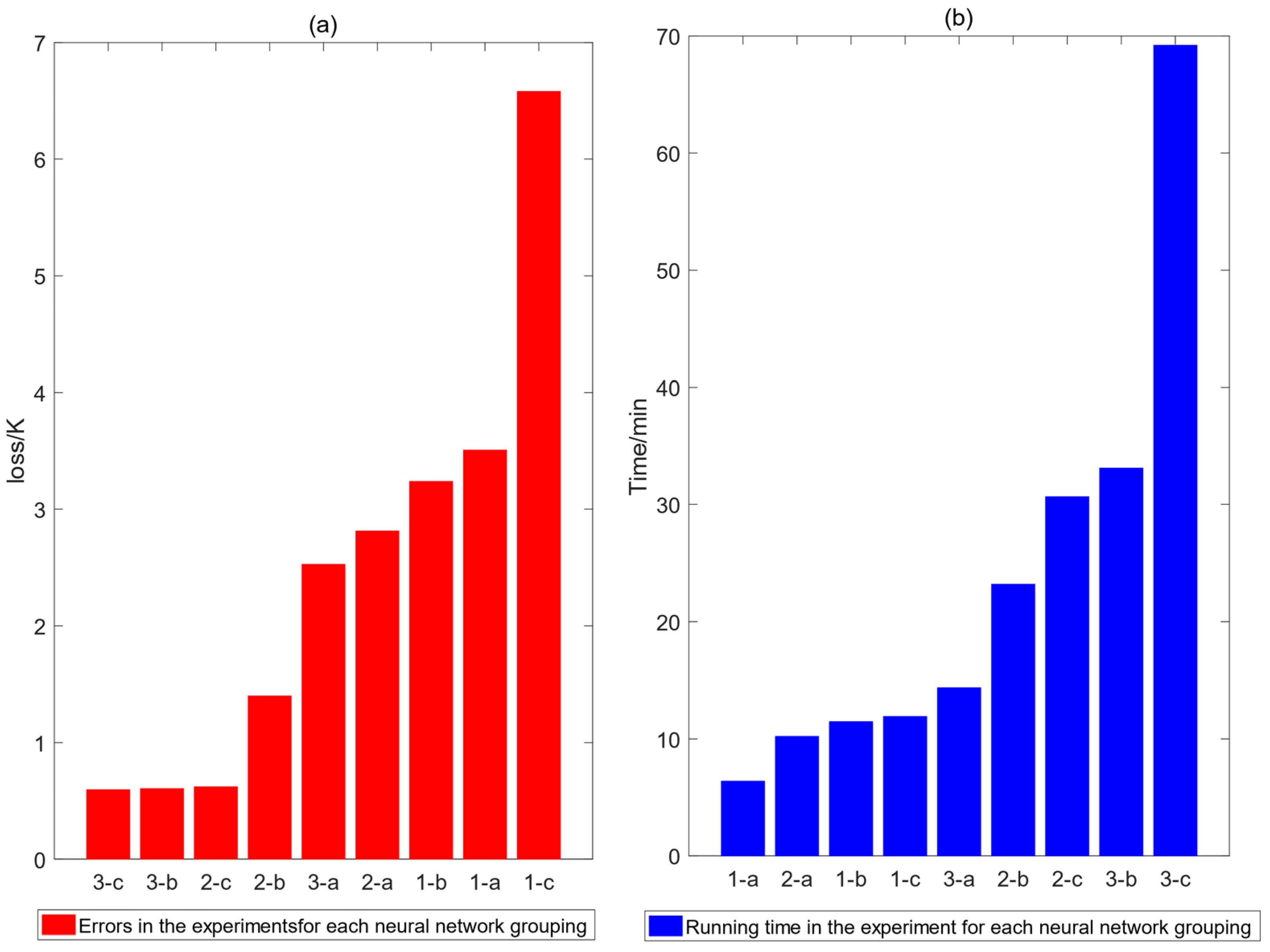
The hardware environment of the finisher is an i9-10900k CPU, an RTX3090 GPU, and 64 GB of RAM. The training method takes the Adam optimization algorithm using the MSE loss function with 4500 iterations and a sample size of 2665 for the training set and 674 for the test set. Experiment 1 used the control variable method. The forecasting time was set uniformly to forecast the eighth day of temperature inversion labeling using seven days of data for three experiments targeting 64, 128, and 256 neurons and 1, 2, and 3 network layers. We obtained suitable configuration parameters for the running time and error by comparing the resultant loss and running time. To facilitate the disclosure of the experimental results, this study rewrote the data 64, 128, and 256 [38] instead of a, b, and c, meaning that a layer of 64 nodes can be expressed as 1-a, and so on.

Based on the above description, LSTM network parameter selection experiments are conducted, and the results are shown in Figure 6.

The analysis shows that for most of the experimental results, for a given fixed dataset, the LSTM network shows a gradual decrease in error and a gradual increase in training time cost as the number of layers and neurons increases. At a deeper level, the improvement in the experimental results, that is, the reduction in error, was more significant and time-consuming with an increase in the number of layers than with an increase in the number of neurons. When the number of neurons in one network layer was 256, the error increased instead of decreasing compared to that with 128 neurons in one layer, which is the most peculiar data in this experiment; this may be because the increase in the number of neuron network layers was insufficiently deep to cause the data to converge.

The three-layer, 256-neuron network obtained the smallest data result (loss). However, compared to the three-layer 128-neuron network, although the error was reduced by 14%, the time cost increased by 108.7%. Considering the efficiency and accuracy of the network, a three-layer, 128-neuron LSTM neural network forecast was selected for further experimentation.

Experiment 2 also used the idea of a control variable comparison test according to the results screened in Experiment 1, in which the forecast model was changed, and 3, 5, 7, and 15 forecast days were compared to screen out the appropriate forecast model. The experiment was conducted based on the experimental design of the previous experiment, and the results are listed in

Table 1. Prediction days and error results from the network parameter experiments.

Three Layers of 128 Neurons
Forecast Days	Loss	Time/h
3	0.4466	1.072
5	0.270993	1.11
7	0.2419	0.995
15	0.0675	1.171
19	0.0689	1.72
30	0.0674	1.83

.

As shown in Table 1, as the number of forecast days increased, the loss at the lowest point decreased gradually. However, the network running time did not show a decreasing trend but fluctuated, centered at 1 h; this is because, with a sufficiently large sample size, the number of forecasts remained numerically close to the initial number of forecast days removed. 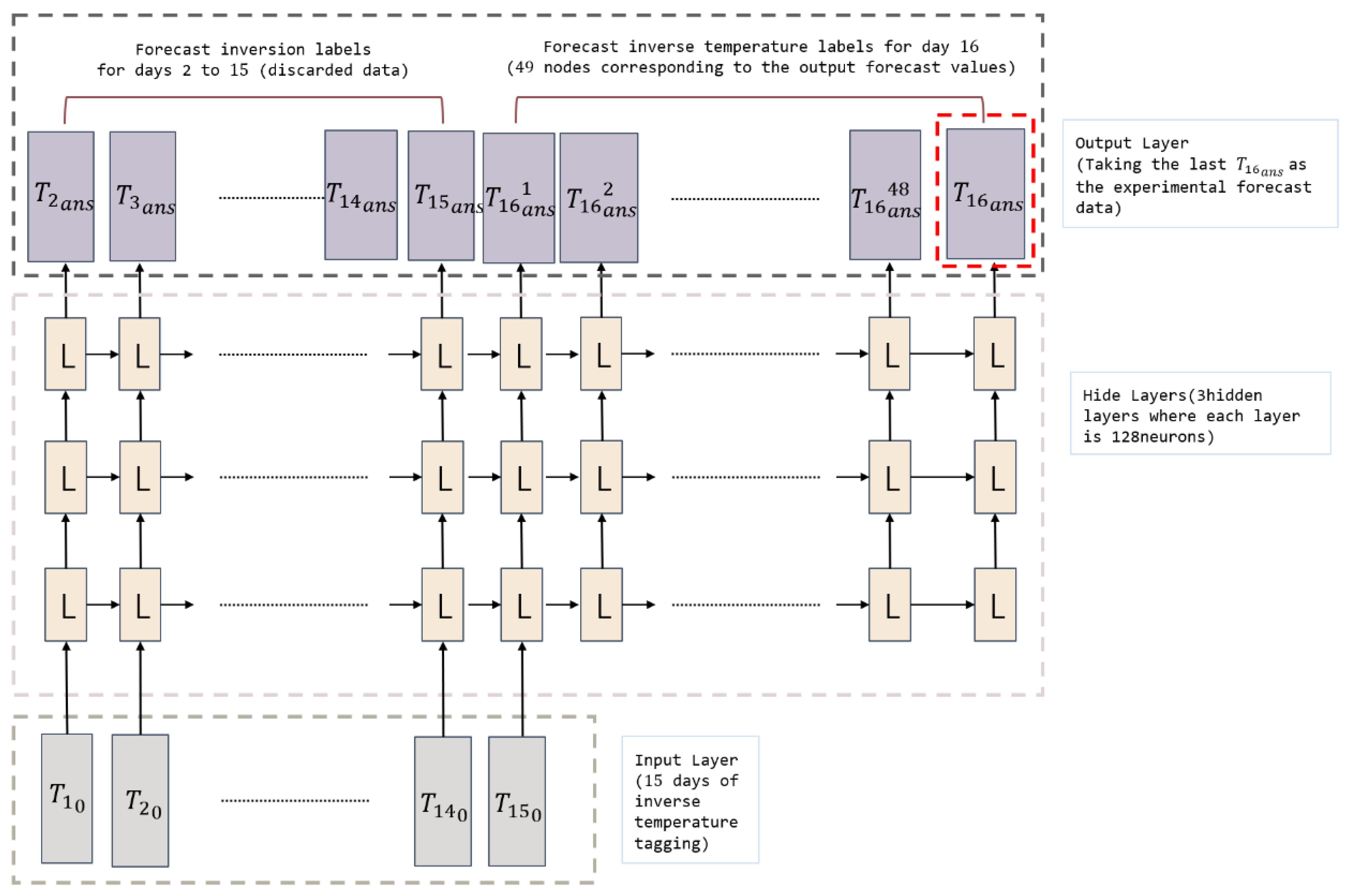Based on the assumption that the minimum error is the optimal network [39], we selected the temperature inversion label $T_n$ for the first 15 d of the LSTM neural network using three layers of 128 neurons to forecast the temperature inversion label of the atmospheric profile on the 16th day. The structure of the obtained LSTM network is shown in Figure 7.

As shown in Figure 7, the temperature inversion labels of day 15 were taken as inputs in each round of rows of this prediction network. The temperature inversion labels of days 2–16 were outputted after three hidden layers, where the prediction outputs for days 2–15 were duplicate terms that were rounded off. The network simultaneously outputs the results of day 16 49 times. Because the error band oscillates and decays according to multiple outputs, the 49th output $T_{{16}_{ans}}$ was taken as the output of the entire network run once.

4. Toroidal Background Field and Forecast Correction Experiments Results and Analysis

A forecast correction algorithm was designed based on the forecast correction model description in the previous two sections. Validation experiments were conducted using seashore data collected in Taizhou from 2013 to 2017. This chapter is divided into two parts. The first part of the experiments verified the calibration ability of the background field expectation profile to the temperature inversion under the temperature inversion condition and without the temperature inversion condition in spring, summer, fall, and winter by comparing the background field data with the inverse data. The experimental results were then analyzed. The second part of the experiment involved a detailed validation of the entire forecast correction algorithm. The experiment imported historical data into the background field to generate the desired profile and generated the temperature inversion label from the desired profile, and the profile was obtained from the radiometer retrieval according to the modified data. The output matrix was obtained by inputting the temperature inversion labels into the LSTM network, and the inversion dataset was linearly summed with equal heights corresponding to the dates to obtain the corrected forecast results. The experimental results were then analyzed.

4.1. Reliability Design Experiments for Expected Background Fields

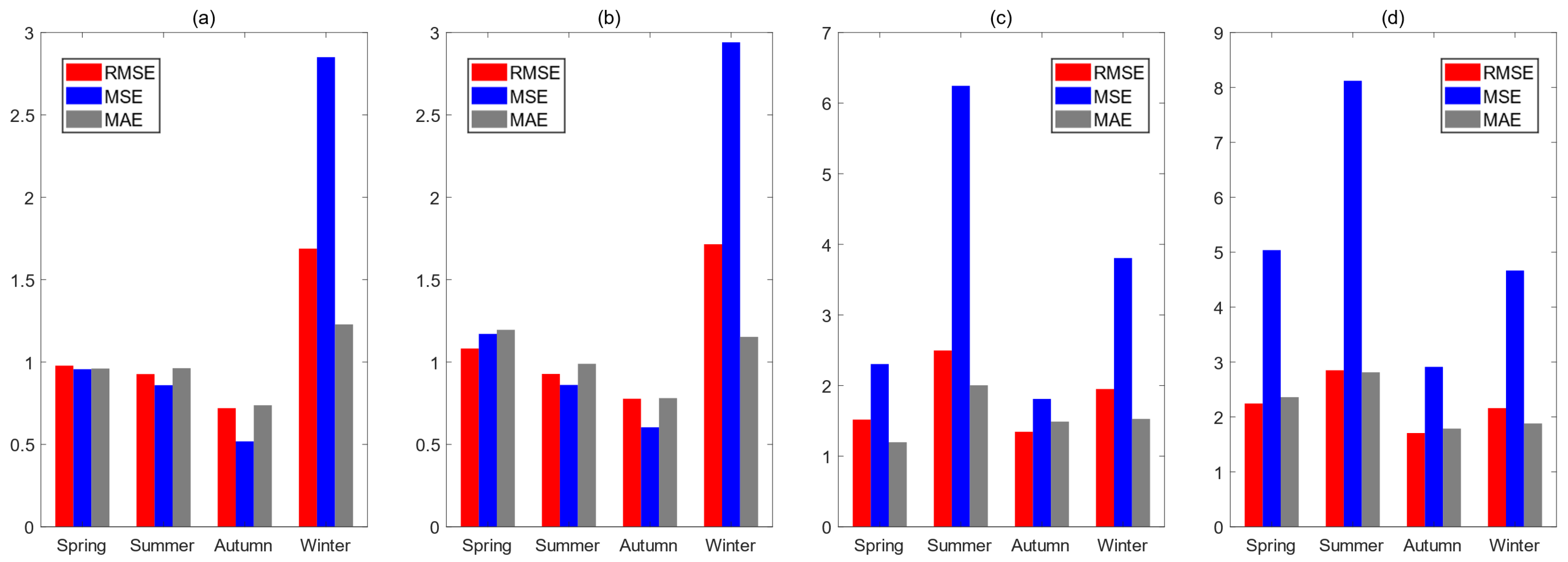
In this round of experiments, the experiments were divided into two groups based on the presence of inversion of temperature in the profile. Each group included two sub-experimental results for background field data, with sounding data as true values, and residual network retrieval data. Each sub-experiment result includes error data under four seasons: spring, summer, fall, and winter. The results of the experiments corresponded to error data, which included root mean square error (RMSE), mean squared error (MSE), and mean absolute error (MAE) values. The experimental results are shown in Figure 8.

As shown in Figure 8, the errors of the retrieval data obtained from the residual network were smaller than the error data of the toroidal background field in all the full-season data. Error fluctuations due to temperature inversion conditions in summer are dramatic. The RMSE and MAE of the residual neural network were reduced by 48.3% and 44.8% compared to the results in the presence of temperature inversion. The RMSE and MAE of the toroidal background field were reduced by 64.9% and 40.8%. The error fluctuation under summer temperature inversion conditions is drastic because the data from the summer profiles are very smooth and fluctuate less during the non-temperature inversion period, leading to lower errors. The inversions are generally influenced by strong convective weather, and the dates of this part of the phenomenon are rare. Hence, tracking both the neural network that uses historical data indirectly and the annular background field that uses historical data directly is difficult. The winter data are the most variable, and little difference exists between the residual network retrieval results and the error data obtained for the toroidal background field under non-temperature inversion conditions. However, regarding the magnitude of the errors, the MSE and MAE data are much higher than the other three seasons by more than 40%.

Meanwhile, the RMSEs of the residual network and the annular background field are 26% and 44% higher, respectively, compared to the data with temperature inversion dates. Although the percentage of error enhancement is not high, the MSE of the residual network and background field reach 3.8056 and 4.6659, respectively. This occurs because a small amplitude of fluctuations already exists in the winter contour of Taizhou, which will produce a large error for the desired contour and retrieval data with smooth values.

The data in this study were collected from Taizhou, a city on the eastern coast of China, which belongs to the central subtropical monsoon maritime climate region [40,41,42], and its climate is characterized by a distinctive change of seasons, which is significantly regulated by maritime factors. The climate pattern of Taizhou is particularly unique in winter [43,44,45], when it frequently experiences strong convective rainfall, a meteorological condition that leads to dramatic fluctuations in the lower atmospheric profile [46,47,48]. The experimental data further reveal that both different atmospheric measurements show a trend of increasing error under inverse temperature conditions. This is mainly due to the fact that the inversion phenomenon breaks the normal temperature gradient of the atmospheric profile, thus increasing the complexity and uncertainty of the measurements. However, it is worth noting that the annular background field shows a unique advantage in reflecting the inverse temperature characteristics. Despite its relatively large error range, the circular background field can more accurately characterize the dynamics and evolution of the inversion process within an acceptable error threshold.

Combining the results and analysis of the above experiments, the annular background field and residual neural network were consistent when the true value of the sounding error was small. Moreover, a temperature inversion occurred at which the height layer of the two could not accurately track the temperature inversion process, and the difference between the true values of the sounding was relatively large. However, because of the range of errors, the annular background field profile in the temperature inversion layer at the temperature inversion profile can better characterize the temperature inversion. Therefore, temperature inversion labeling is more prominent. Thus, the desired background field $E\left[S_{(t,h)}\right]$ calculated according to the uniformly distributed annular background field can play the role of accurate calibration in the temperature inversion label calibration.

4.2. Comparative Analysis of Temperature Inversion Correction Based on Forecast Results

Vertical resolution is an important index in the field of microwave remote sensing [49], so the method proposed in this paper also improves the vertical resolution of microwave remote sensing data.

Table 2. Vertical resolution comparison of different retrieval algorithms.

Vertical Resolution of Microwave Radiometer MP3000A Based on NN Network
Altitude (m)	100	200	500	1000	2000	5000	10,000
Vertical resolution (m)	50	50	100	100	250	250	250
Vertical Resolution of Microwave Radiometer MP3000A Based on the Proposed Network
Altitude (m)	100	200	500	1000	2000	5000	10,000
Vertical resolution (m)	100	100	100	100	100	100	100

shows the resolution of the initial radiometer network and the resolution of the improved method. The output vertical resolution of the residual neural network used in this paper is 100 m, which is higher compared to the vertical resolution of the traditional NN network of MP3000A.

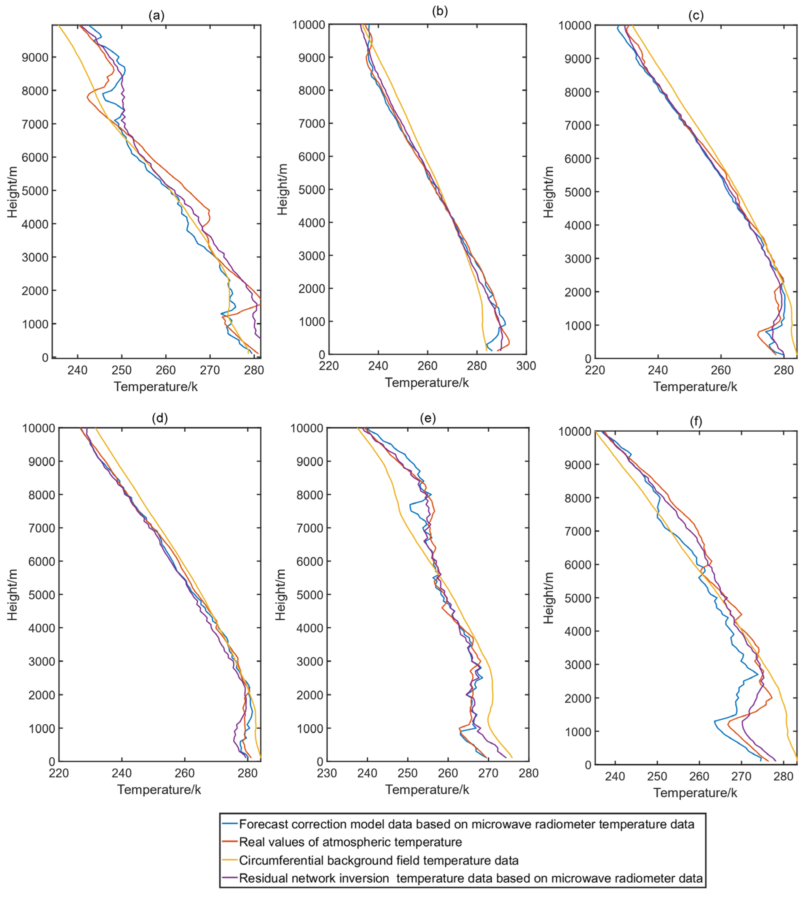
In addition, the previous round of experiments confirmed that the background field could be calibrated to the temperature inversion within a certain error. This round of experiments used a forecast correction algorithm for the validation experiments. The experiment was divided into two groups. The first group of experiments used dates when the temperature inversion existed, and the second group used dates when the temperature inversion was weak or almost non-existent. The background field, retrieval, correction, and real-sounding data were compared during the experiments. 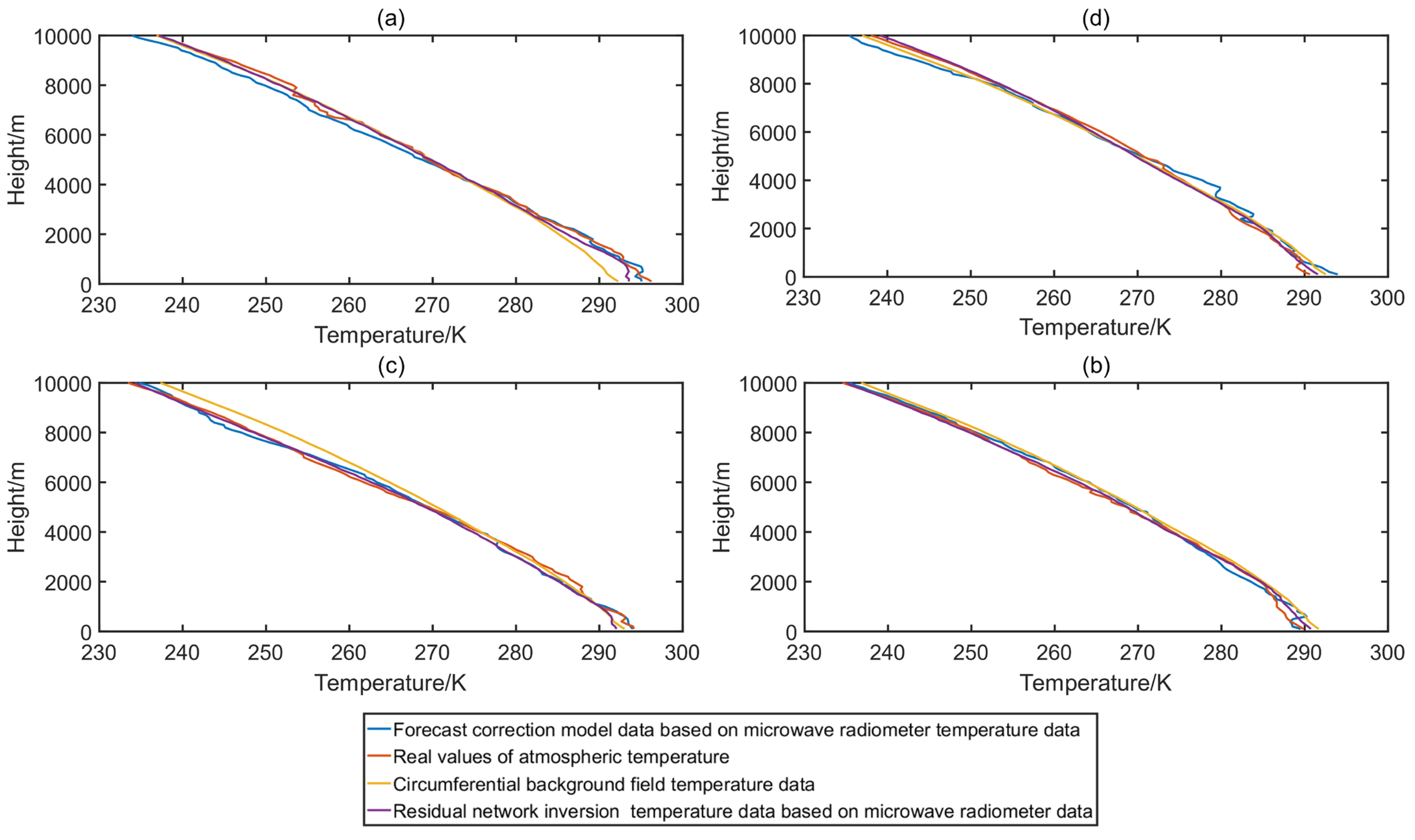The results of the first set of experiments are shown in Figure 9.

Figure 9a,b correspond to profile numbers 64 and 1399 in the forecasting experiments. As shown in Figure 9a, in the temperature inversion region above 8000 m, the RMSE of the residual neural network was 5.74 and 2.01, and the RMSE of the residual neural network corrected by the addition of the forecast results was 3.39 and 0.99, which was 40.9% and 50.7% less than that before correction. For profiles from group 1399 with profiles below 2000 m, the residual neural network RMSE was 1.77, which represents a reduction of 3.52 from the previous correction. The time lag of the label correction caused this increase in the RMSE.

The serial numbers 1411 and 1412, corresponding to Figure 9c and Figure 9d, respectively, exhibit two sets of date-adjacent spring profiles in Taizhou, a city characterized by its subtropical monsoon climate with distinct seasons and significant oceanic influence. During the spring season, as derived from the background field profiles, some inversions emerged in the low-level atmosphere over Taizhou. These inversions are typical meteorological phenomena influenced by the interplay between warm and cold air masses, often exacerbated by topographical features and sea–land breezes. Meanwhile, the circumferential background field profiles remained relatively stable due to the temporal proximity of the measurement dates.

On both days, substantial inversions beyond the range of normal background field fluctuations were observed in the near-surface lows, largely attributed to the monsoon winds that bring about significant changes in temperature and wind direction. The inversion in profile No. 1411 was particularly intense. When correcting for this inversion using a residual neural network, the root mean square error (RMSE) below 2000 m was 2.56. By incorporating the forecast result into the correction, the RMSE decreased to 2.38, a 7.0% improvement. For the neighboring day’s profile 1412, the RMSE of the residual neural network, after incorporating the forecast correction, was reduced to 1.51, a 24.1% decrease compared to pre-correction. Overall, the RMSEs before and after correction were 1.71 and 1.09, respectively, marking a 36.3% reduction in this experiment. The correction was particularly effective for profile 1412, which exhibited smaller temperature inversion fluctuations, indicating that for low-altitude inversions, corrections are more accurate when profiles are closer to the background field.

For winter profile numbers 23 and 24, corresponding to Figure 9e and Figure 9f, respectively, the true value profiles oscillate significantly due to the convergence of the Siberian cold front and the Pacific warm front. This meteorological condition is typical of Taizhou’s winter, where the city experiences drastic temperature changes and strong winds as cold and warm air masses clash. The background field struggled to track the sounding data at both near-surface low and high altitudes under such extreme weather conditions. However, when using ResNet and its forecast correction, more accurate tracking became possible. The RMSE of the residual neural network was initially 2.95 but dropped to 1.27 after incorporating the forecast correction, representing a remarkable 56.9% reduction. This underscores the residual neural network’s ability to maintain high correction accuracy even under conditions of violent profile fluctuations.

In summary, the analysis of these profiles not only demonstrates the efficacy of using neural networks for correcting atmospheric inversions but also highlights the unique climatic challenges faced by Taizhou, particularly during the transition seasons when monsoon winds and temperature inversions are prevalent. By understanding these challenges and leveraging advanced data correction techniques, we can improve the accuracy of weather forecasts and climate models, thereby enhancing our ability to mitigate the impacts of extreme weather events.

The second set of experimental results was for the experiments conducted for dates with almost no temperature inversion phenomenon. The results of the experiments are shown in Figure 10.

The profile forecast correction based on the residual network was also more accurate than the original residual retrieval network in the case of small or almost no temperature inversions. The RMSE of the residual network with the addition of the forecast result correction was improved by 6% in experiments 1512, 1516, 1518, and 1522 relative to that of the residual network without correction. For minor inversions, the residual networks had higher accuracy with fewer errors. Meanwhile, because of the lack of the temperature inversion phenomenon in the atmospheric conditions on that day, the value of the temperature inversion prediction label output by the LSTM network was small; this is exemplified by the last round of experiments on the toroidal background field, where the results of the residual network retrieval in the non-temperature inversion state were kept at a very low error level. Therefore, even after adding the residual network with the correction of the forecast result, the reduction in the error embodied in the numerical value was not obvious.

For the full data based on the time series, error variation is shown in Figure 11.

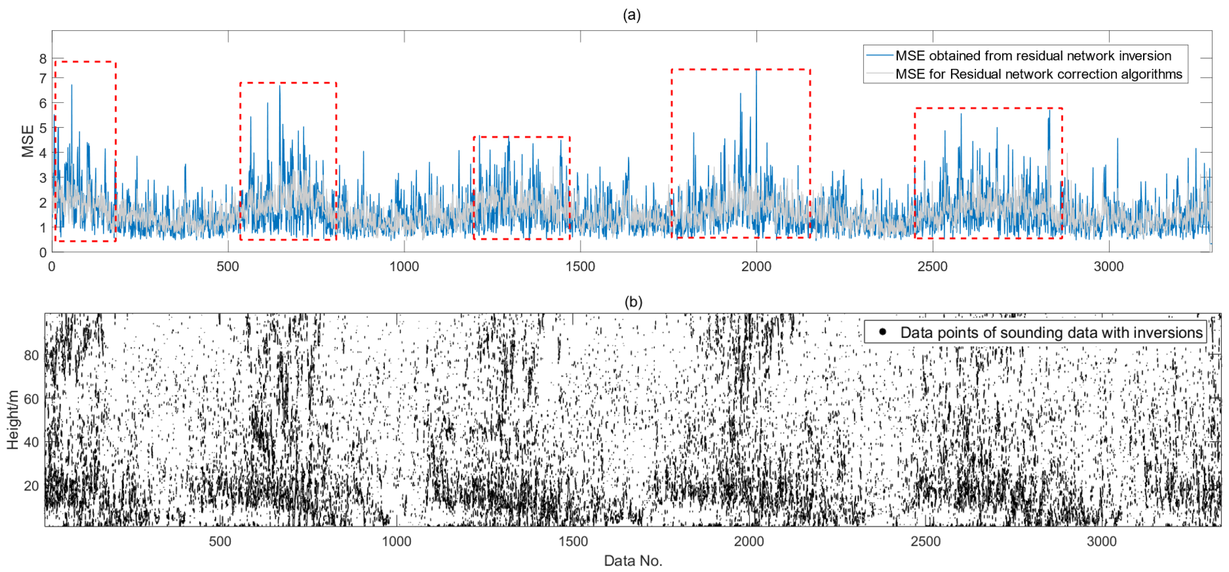
It can be intuitively obtained from Figure 11 that the error bands of the forecast correction algorithm are significantly more convergent than the residual network. The improved algorithm produces a substantial reduction in intra-adjacent data errors. Among the error bands with 95% data coverage, the forecast correction algorithm reduces the error range band by 33% compared to the residual network. The red rectangular region represents the region where the error of the inversion results of the residual network shows large fluctuations. Also, the region of frequent inversions in panel (b) coincides with the region in the red box in panel (a). These error fluctuations positively correlated with the temperature inversion phenomenon affect the error bands of the residual network negatively, which greatly increases the range of the error bands and the instability of the inversion results under the temperature inversion phenomenon; this indicates that the algorithm proposed in this study can effectively improve the stability of the inversion data under the temperature inversion phenomenon.

For all the data in the corrected experimental results, error data is as follows in

Table 3. Forecast the error results of the comparison tests of the correction model and the residual network, where the error data include MSE data and MAE data.

Comparison of MSE Data for Corrected Experimental Results
Inversion of Temperature	Residual Network Data	Forecast Correction Model Experimental Data
Existence	3.245	2.166
Non-existent	1.711	1.643
Comparison of MAE Data for Corrected Experimental Results
Inversion of Temperature	Residual Network Data	Forecast Correction Model Experimental Data
Existence	1.735	1.511
Non-existent	1.108	1.098

.

As shown in Table 3, for the dataset with the temperature inversion in the experiment, the MSE of the residual network with sounding data as the true value was 3.245. Meanwhile, the forecast correction algorithm obtained 2.166. The findings have demonstrated that the background field profile could be used to calibrate the temperature inversion-warming phenomenon within the error range. The LSTM forecast correction network based on this background field shows a 34% reduction in the temperature inversion condition error; at the same time, the MAE error was reduced by 13%. For the dataset with almost no inversions in the experiment, the MSE of the residual network using the sounding data as the true value was 1.711.

Meanwhile, the forecast correction algorithm obtained an MSE of 1.643. Therefore, the forecast correction algorithm reduced the error by 4% for the overall range of data in which inversions were present. Within the data range, the network had an extremely limited effect on improving radiometer retrieval accuracy in small or almost non-existent temperature inversions.

5. Conclusions

Accurate inversion of atmospheric temperature using bright temperature is important for environmental monitoring, aerospace, and weather forecasting. Therefore, it is of considerable meteorological importance to improve the accuracy of atmospheric temperature observations in the near-surface troposphere. Under suitable meteorological conditions, a microwave radiometer can invert the atmospheric temperature profile from 0 to 10 km with a relatively high level of accuracy. However, as non-contact remote sensing devices, microwave radiometers produce large errors when the temperature inversion phenomenon occurs. To address this problem, this study proposed a forecast correction model based on an LSTM network with a circumferential background field. The model first constructs a toroidal background field by regressing the local atmospheric temperature in Taizhou. Then, temperature inversion labels were generated using the data obtained from the annular background field and radiometer retrieval. Correction results were obtained by linearly summing the temperature inversion labels and inversion data. The method utilizes a combination of statistically distributed background fields and neural network forecasting. Compared to a single neural network algorithm, the method utilizes historical data more systematically based on statistical regression and is compatible with the advantages of rapid and accurate LSTM network forecasting. In addition, the correlation algorithm proposed in this paper improves the vertical resolution of the radiometer compared to the initial algorithm that comes with the MP3000A microwave radiometer. Validation experiments were also conducted using climate data from the Taizhou seaside collected over five years. The following conclusions were drawn from the experiments:

• The annular background field generated based on the local climate distribution of Taizhou was within the error range and could stably output temperature inversion labels in the presence of the temperature inversion phenomenon.
• The experiment demonstrated that the three-layer, 128-neuron LSTM neural network could more accurately use the temperature inversion labels of the first 15 days to forecast the atmospheric profile temperature inversion labels of the 16th day based on a loss accuracy of 0.0675.
• The algorithm proposed in this study under the temperature inversion phenomenon can effectively improve the stability of the retrieval data. In the data range, the error band range is reduced by 33% in the temperature inversion condition compared with the residual network.
• The forecast correction algorithm based on the annular background field can reduce errors from radiometer inversion in the presence of inversions. The MAE was reduced by 34% across all data ranges. In the non-temperature inversion condition, the effect of the network on the accuracy of the radiometer retrieval was extremely limited, and the MAE was reduced by only 4%.

The toroidal background field tracked the inversions slightly too well within the error range. The LSTM network predicted the inversion labels more accurately within a certain accuracy range, and the forecast corrections were more accurate under stronger inversions closer to the desired background field profile. It also accurately tracked the inversions at near-surface lows and highs for strong inversions when the profile fluctuations were relatively prominent. The results were more accurate for strong inversions with pronounced profile fluctuations. However, in the case of small and no inversions, the results of the forecast correction were still due to the residual network, although the numerical representation was not obvious. Overall, this method improved the accuracy of the neural network retrieval of atmospheric profiles.

However, this study had certain limitations. Due to the insufficient time span of the data, no observations of more than ten years were obtained, and the forecasting effects on large time scales could not be effectively verified. Meanwhile, the circular background forecast correction model was based on historical data in the forecasting process. Therefore, the model could not track the temperature profile fluctuations caused by large extreme climate changes on neighboring dates. In addition, the method is proposed based on neural networks, which are typical black-box structures; it is difficult to interpret systematically. At the same time, LSTM networks have insufficient forecasting ability for irregular missing time series data. Therefore, we will focus on solving the effect of large-scale climate fluctuations on the accuracy of radiometer inversion and the problem of neural network interpretability in the future.