A Deep Learning Method for Inversing 3D Temperature Fields Using Sea Surface Data in Offshore China and the Northwest Pacific Ocean

Abstract

Three-dimensional ocean temperature field data with high temporal-spatial resolution bears a significant impact on ocean dynamic processes such as mesoscale eddies. In recent years, with the rapid development of remote sensing data, deep learning methods have provided new ideas for the reconstruction of ocean information. In the present study, based on sea surface data, a deep learning model is constructed using the U-net method to reconstruct the three-dimensional temperature structure of the Northwest Pacific and offshore China. Next, the correlation between surface data and underwater temperature structure is established, achieving the construction of a three-dimensional ocean temperature field based on sea surface height and sea surface temperature. A three-dimensional temperature field for the water layers within the depth of 1700 m in the Northwest Pacific and offshore China is reconstructed, featuring a spatial resolution of 0.25°. Control experiments are conducted to explore the impact of different input variables, labels, and loss functions on the reconstruction results. This study’s results show that the reconstruction accuracy of the model is higher when the input variables are anomalies of sea surface temperature and sea surface height. The reconstruction results using the mean square error (MSE) and mean absolute error (MAE) loss functions are highly similar, indicating that these two loss functions have no significant impact on the results, and only in the upper ocean does the MSE value slightly outperform MAE. Overall, the results show a rather good spatial distribution, with relatively large errors only occurring in areas where the temperature gradient is strong. The reconstruction error remains quite stable over time. Furthermore, an analysis is conducted on the temporal-spatial characteristics of some mesoscale eddies in the inversed temperature field. It is shown that the U-net network can effectively reconstruct the temporal-spatial distribution characteristics of eddies at different times and in different regions, providing a good fit for the eddy conditions in offshore China and the Northwest Pacific. The inversed eddy features are in high agreement with the eddies in the original data.

1. Introduction

The three-dimensional temperature fields play a vital role in oceanography research [1], and their vertical distribution determines the location of characteristic structures such as the oceanic mixed layer, thermocline, and barrier layer [2,3]. The three-dimensional ocean temperature fields have a significant impact on air–sea interactions, ocean circulation, and climate change [4,5]. Furthermore, the temperature information of seawater is also an important influencing factor of ocean phenomena [6,7] The change in subsurface temperature can cause changes in the ocean’s heat budget, which in turn affects the occurrence and dissipation of ocean phenomena [8]. The subsurface temperature of the ocean is also one of the key indicators of climate change [9,10].

An accurate understanding of the three-dimensional ocean temperature structure is crucial for oceanographic research. At present, there is an urgent need for continuous and high spatiotemporal resolution three-dimensional ocean data, and the most effective way to obtain such data is through in situ observations. Observations of ocean data are typically conducted using observation methods such as scientific expedition vessels and Argo. However, in situ observation methods do not provide real-time descriptions of the changes in the internal temperature structure of the ocean due to the discrete data. Numerical simulation methods obtain marine environmental data by establishing regional models but are generally applicable to specific sea areas and are limited in that they greatly increase the demand for computational resources, making it difficult to achieve operational applications. With the development of ocean satellite technology, there has been a tremendous increase in sea surface observation data. Unfortunately, it is difficult for ocean remote sensing observations to penetrate the sea surface to shed light on the temperature structure changes underwater, and the vast majority of ocean dynamic processes are not limited to the surface, usually extending to a depth of thousands of meters underwater. Therefore, ocean remote sensing data cannot provide us with comprehensive ocean information, and how to obtain ocean data of the meso-micro scale remains a problem in oceanography research. Sea surface temperature may affect the temperature of deep layers, while the latter may cause changes in seawater density, in turn leading to changes in sea surface height. If a correlation can be established between sea surface data and underwater data, then inversely reconstructing the underwater environment using sea surface data to obtain relevant underwater data will help us gain a more comprehensive understanding of ocean processes.

The current methods for reconstructing the underwater temperature field based on sea surface data mainly include statistical methods [11], dynamic models [12], and artificial intelligence (AI) methods [13]. Statistical methods are used to establish the correlation between sea surface variables and underwater parameters through mathematical statistics. Such methods are suitable for research in ocean areas where the ocean dynamics are quite stable, but for areas with more complex environments, the reconstruction results tend to have greater errors. Dynamic models have been developed based on the theory of ocean variation, using idealized dynamic equations to establish the relationship between sea surface variables and underwater parameters. Although such methods can, to some extent, reflect the actual background of the ocean, the constructed models are typically only applicable to specific sea areas and are difficult to apply accurately for the reconstruction of temperature fields in all periods and sea areas. In recent years, the rise of AI has provided new ideas for the reconstruction of ocean temperature fields. AI models can accurately reconstruct the underwater temperature field by learning the relevant characteristics between the sea surface and underwater temperature. AI methods mainly include traditional machine learning and deep learning methods.

Traditional machine learning methods include support vector machine (SVM), support vector regression (SVR), random forest (RF), additive models based on boosted trees, and lightweight gradient boosting machines. Lu et al. [14] proposed an SVM method that employed observation data from Argo to inversely reconstruct the sea temperature anomaly (STA) in the Indian Ocean, with sea surface temperature anomaly (SSTA), sea level anomaly (SLA), and sea surface salinity anomalies (SSSA) as input variables of the model. Lu et al. [14] also used the extreme gradient enhancement method to reconstruct the global three-dimensional temperature field anomaly by taking sea surface temperature (SST), sea surface high (SSH), and sea surface salinity (SSS) data, and sea surface wind field (USSW, VSSW) as input variables and compared the results with Argo data to verify the accuracy of the model reconstruction.

With the development of deep learning models, such methods have increasingly been applied in the field of ocean research. The commonly used deep learning methods for reconstructing the ocean temperature field include convolutional neural networks (CNNs), generative adversarial networks (GANs) [15], self-organizing maps (SOMs), and hybrid models that combine several neural networks. Ali et al. [16] used neural networks to invert deep ocean thermal structures through sea surface information, with most errors controlled within 1 °C. Han et al. [17] conducted a study on the reconstruction of the three-dimensional temperature field in the Pacific Ocean based on SST, SSH, and SSS data using a CNN model. They established temperature reconstruction models for different months and verified the accuracy of the reconstruction results with Argo observation data. The results showed that the CNN model could accurately reconstruct the three-dimensional underwater temperature field in the Pacific Ocean, with root mean square errors ranging from 0.26 to 0.52 °C. The study also found that in the upper layer from 0 to 300 m, the temperature field changed significantly, and the accuracy of the reconstructed temperature field began to decrease below a depth of 500 m. Su et al. [18] employed CNN and Light GBM models, leveraging satellite remote sensing data in conjunction with Argo buoy observation data and EN4 profile data, to reconstruct a high-resolution global three-dimensional ocean temperature field above 1000 m, with a resolution of 0.25 × 0.25°. They used SST, SSH, SSS, USSW, and VSSW data and compared the differences in the reconstruction results between the two methods. The Light GBM and CNN reconstruction results showed that the RMSE generally first increased, then decreased with increasing water depth. In the case of a large amount of input data, the reconstruction accuracy of CNN was higher than that of Light GBM. Meng et al. [19] proposed a method for predicting underwater temperature fields based on a combination of GAN networks and numerical models. First, they used the GAN model to learn the physical relationship between sea surface data and underwater parameters in the numerical model, then calibrated the model using Argo data to enhance its inversion performance. Next, they used HYCOM reanalysis data to train the GAN model and Argo and National Oceanic and Atmospheric Administration (NOAA) data to adjust the model parameters, then reconstructed the three-dimensional temperature field of the South China Sea region. The results suggested that the GAN network performed well in reconstructing the three-dimensional temperature field. Wang et al. (2021) [20] proposed an improved neural network model to estimate the ocean subsurface thermal structure from 0 to 2000 m from multisource sea surface data, including SST, SSS, SSH, and sea surface wind. Compared with the random forest (RF), the multiple linear regression (MLR), and the extreme gradient boosting (XGBoost), the proposed model outperformed these models. Liu et al. [21] proposed a DL-based mesoscale eddy subsurface temperature inversion model, with which study observations and satellite sea surface ones (sea surface height, sea surface temperature) are combined to develop the inversion model of the subsurface temperature. Zhang et al. [22]. Proposed a new method to invert ST from the sea surface information in China’s marginal seas based on the generative adversarial network (GAN) model, which can project the STs from sea surface information (SLA, SSTA, SST) with a high resolution of 1/12°. Despite sufficient research on ocean temperature in previous studies, there is still a lack of advanced models for inversion and analysis of ocean phenomena. Sammartino et al. [23] used ANN to inverse temperature, and it can obtain good results.

The research area of this article is 10° S–55° N, 100° E–165° E. The Northwest Pacific and offshore China are part of the Northern Pacific Ocean. As one of the largest regions of the Pacific, the temperature structure of the Northwest Pacific and offshore China is influenced by various cyclones [24] and monsoons, with pronounced seasonal changes in the marine environment [25]. The vast maritime space is also conducive to the occurrence and evolution of mesoscale eddies and other ocean dynamic processes, due to the frequent small- and medium-scale dynamic activities there [26,27,28,29]. However, due to the lack of in situ data, research on mesoscale eddies remains in the exploratory stage. Therefore, it is necessary to reconstruct the three-dimensional temperature field of the ocean. Previous models mostly used simple CNNs, which had poor ability to extract image details. The U-net network has a special structure for image segmentation and possesses a stronger ability to extract image information. Therefore, in the present study, the three-dimensional temperature structure of the Northwest Pacific and offshore China is reconstructed and verified through sea surface information inversion using a U-net network.

2. Data and Methods

2.1. Data

The ocean data used in this paper are Global Ocean Reanalysis and Simulation (GLORYS12V1) reanalysis data. The GLORYS12V1 ocean reanalysis dataset is adopted, which is a product of the Copernicus Marine Environment Monitoring Service (CMEMS) global ocean eddy resolution reanalysis (with a spatial resolution of 1/12°, temporal resolution of 1 day, and 50 vertical layers), covering altimeter data (after 1993). The product delivers daily average data for temperature, salinity, sea level, and mixed layer depth [30].

With the data of sea surface parameters as the input data for model training and underwater data as the label data for the reconstruction of the three-dimensional temperature field, the temperature structure of various depth layers is marked and the accuracy of the reconstruction results is determined. Before inputting the sea surface variables and label data into the model, all sample data must be preprocessed. First, the spatial resolution of the sea surface input data and subsurface temperature data must be unified. Through nearest neighbor interpolation (1), the spatial resolution of the GLORYS reanalysis data is interpolated to a 0.25 × 0.25° grid, with a temporal resolution of 1 day ($x$ and $y$ are interpolated values, $x_i$ and $y_i$ are raw data).

$$y=y_j where j=\arg \underset{i}{\min }|x-x_i|$$

(1)

Next, the dataset of the temperature field reconstruction model is divided. The data used in this study span from 1 January 2010 to 31 December 2018, totaling 3357 samples. Of these, 2992 samples from 2010 to 2017 are used to train the model and optimize the reconstruction parameters and are divided into training and validation sets in an 8:2 ratio. The temperature data from 2018 are used as the test set to evaluate the model’s accuracy in reconstructing the subsurface temperature structure of the ocean.

The main goal of this experiment is to explore the impact of different processing methods and loss functions for sea surface data on the reconstruction of the underwater temperature field. The input data for the model are obtained through different processing methods. Specifically, for the reconstruction of the underwater temperature field, the reconstruction results of the original values and the anomalies as input variables are compared. The original values are the SST and SSH data after interpolation in the GLORYS reanalysis data. The anomalies are the SSTA and SLA obtained by subtracting the mean of the original values from the original values. The calculation formulas are as follows:

$$SSTA=SST-SS{T}_{mean}$$

(2)

$$SLA=SSH-SS{H}_{mean}$$

(3)

Additionally, considering the differences in magnitude among various variable data, a unified normalization process is required to prevent these differences from affecting the accuracy of the reconstruction results before the data are input into the model. In this way, different variables are at the same magnitude and dimension and are distributed within the same range of values. The normalization expression is as follows:

$$X={\displaystyle \frac{x-\mu }{\sigma }}$$

(4)

where $x$ represents the initial value of the sea surface variable in all data; $\mu \mathrm{a}\mathrm{n}\mathrm{d} \sigma$ are their mean and standard deviation, respectively; and $X$ is the normalized sea surface variable. After normalization, all sea surface variables are concentrated within a numerical range with an average value of 0 and a variance of 1.

After normalizing all input variables, the terrain is further processed as a Not a Number (NaN) value. Previous experiments have shown that setting the NaN value to 0 may minimize the interference of the NaN value on the reconstruction results. In this study, after comparing the results of multiple experiments, the NaN value related to the land is set to 0.

2.2. Method

In this paper, the U-net [31] network is selected for the reconstruction research of the three-dimensional temperature field. The structure of the U-net network can preserve more data details and extract contextual information for feature fusion. U-net is an improved fully convolutional network that takes an image or a complete data matrix as input and, through symmetric upsampling and downsampling processes, outputs a result of the same size as the input data. U-net is mainly applied for image segmentation tasks and has been widely applied in the field of biomedical image segmentation since 2015. It is an end-to-end semantic segmentation network and was initially valued for its ability to effectively address biomedical problems. Thanks to the effectiveness of U-net architecture in solving image-to-image mapping tasks, it is chosen to serve as the basis for constructing our model. While the encoder part extracts features from the input image, the decoder part performs classification on each pixel to reconstruct the segmented output. Plus, a set of residual connections between both parts allows a precise localization in the output image [32].

The network structure of this study was built using the TensorFlow library in Python language. As shown in Figure 1, a U-net is a symmetrical encoder–decoder structure and is named for the model’s U-shape, which is mainly divided into two parts: the encoder and the decoder. The structure on the left-hand side is the encoder, which comprises convolutional and pooling layers. Its main functions are downsampling and pooling, and it is primarily used for feature extraction. It is divided into multiple layers, where the input data are downsampled through a series of convolutional and pooling layers to gradually reduce resolution. The encoder captures advanced features of the input data; in this way, through convolutional operations, the model can learn the local features within the data. The right-hand part is the decoder, where the input data are gradually restored to their original spatial resolution through a series of upsampling and deconvolution operations. The function of the decoder is to generate prediction results based on the advanced features provided by the encoder. Its structure resembles that of the encoder, the difference being that the decoder employs deconvolution operations to gradually increase the resolution of the data. Additionally, there are fully connected layers in the U-net network, encompassing the structure of a bridge and skip connections. The bridge is a channel connecting the encoder and decoder, and its function is to preserve advanced feature information so that it can be used in the decoder to more accurately restore details and shapes. The bridge connections ensure that the decoder has sufficient contextual information when generating predictions since the last few layers of the encoder typically contain information regarding the overall image structure. The skip connections are direct links from a certain layer of the encoder to the corresponding layer of the decoder. Such connections preserve feature maps of higher resolution, thus helping to refine the segmentation results. Through these connections, the model can integrate information at different scales, thereby better capturing local details and global context. Skip connections also help alleviate the problem of gradient vanishing, because through them gradients can be more easily passed back to earlier layers. Both direct and skip connections are designed to address the issues of information loss and gradient vanishing, enabling the U-net network to simultaneously utilize advanced abstract features and detailed information.

Compared to simple CNN models, the U-net network has a special structure for image segmentation. The skip connection structure in the model can effectively mitigate the vanishing gradient problem during training. Moreover, CNN models have a high demand for data volume during training. In contrast, the U-net network requires less data, allowing it to achieve more accurate training results with less data input. Therefore, in this paper, the U-net network is adopted to achieve the reconstruction of the three-dimensional temperature field in the study area.

2.3. Loss Function

Loss functions are computational functions that measure the discrepancy between a model’s predicted and actual values. They serve as important criteria for evaluating the quality of the output results. A loss function is a non-negative real-valued function, and in deep learning computation, a smaller loss function means the model fits the data well.

Loss functions are used during the model training phase. After each batch of training data is fed into the model, the predicted value is output through forward propagation, then the loss function calculates the difference between the predicted values and the actual values, i.e., the loss value. Once the loss value is obtained, the model updates its parameters through backpropagation to reduce the discrepancy between the predicted and actual values. This process aligns the model’s predictions more closely with the actual values, achieving the goal of learning.

In this experiment, the Mean Absolute Error (MAE) and Mean Squared Error (MSE) loss functions were used.

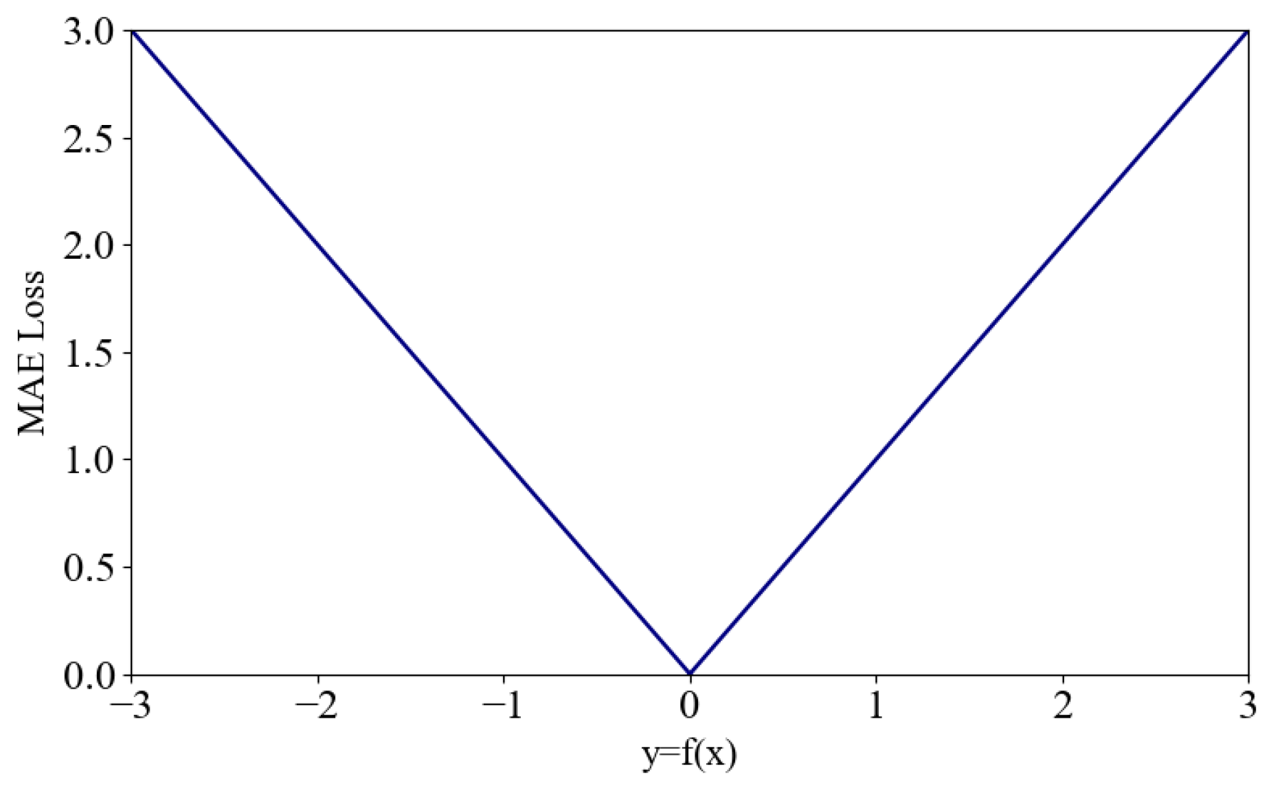
(1) MAE loss function

The principle of calculating the MAE loss function is to take the average absolute value of the difference between the estimated and actual values (Figure 2):

$$\mathrm{MAE}={\displaystyle \frac{1}{n}}{\displaystyle {\sum }_{i=1}^n}|f(x_i)-y_i|$$

(5)

where $f\left(xi\right)$ is the output value of the model, and $y_i$ is the actual value. When the two are the same, the MAE loss reaches its minimum value, which is 0. Then, as the difference between the output value and the actual value increases, the MAE loss value shows a linear growth trend.

Although the MAE curve is continuous, it is not differentiable at $f(x_i)-y_i=0$. In most cases, the gradient of the MAE loss is the same, which is not conducive to rapid convergence.

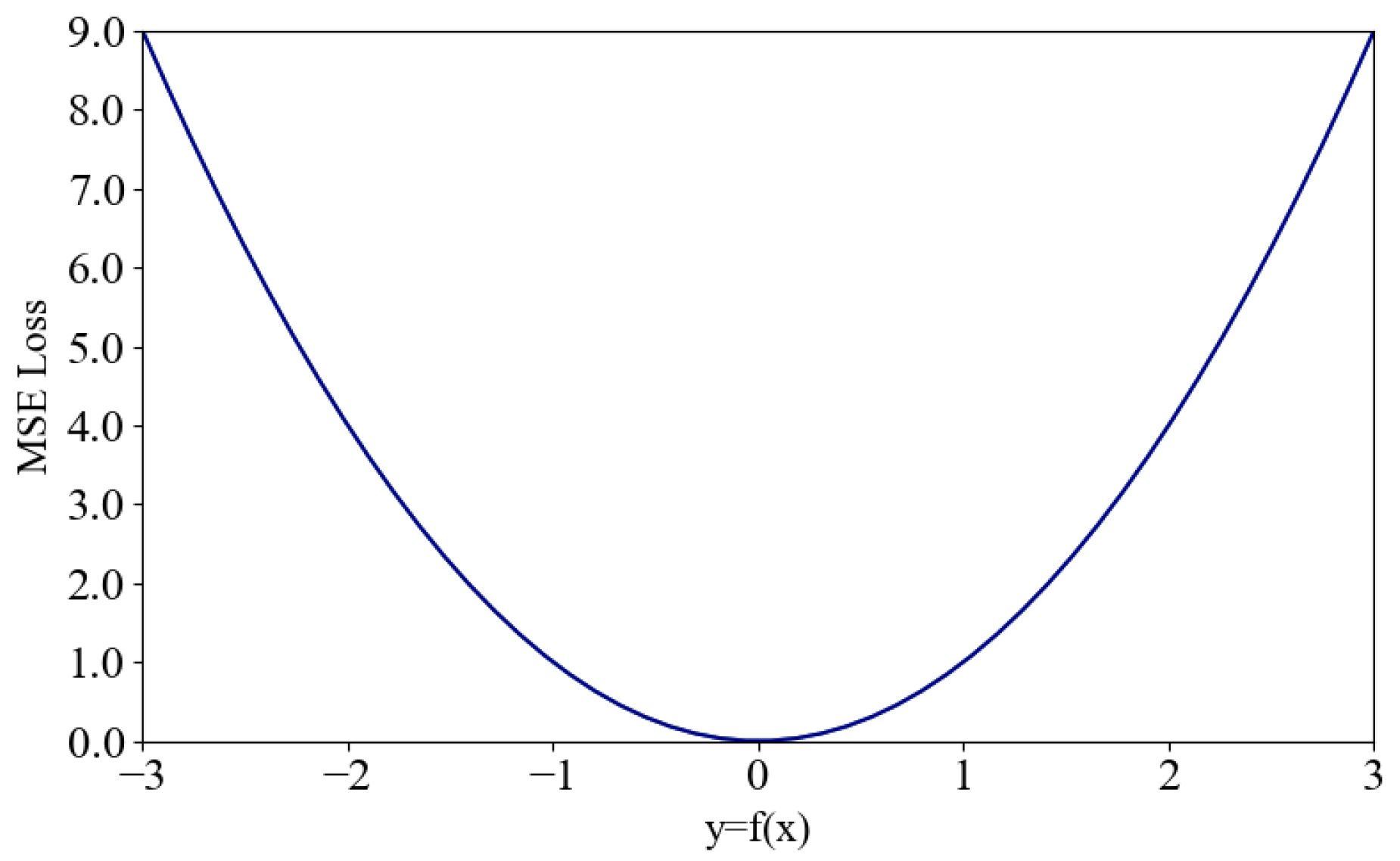
(2) MSE loss function

The principle of calculating the MSE loss function is to take the average of the sum-of-squared difference between the estimated value and the actual value (Figure 3).

$$\mathrm{MSE}={\displaystyle \frac{1}{n}}{\displaystyle {\sum }_{i=1}^n}{(f(x_i)-y_i)}^2$$

(6)

The figure shows that MSE is a smooth function differentiable everywhere and aids in calculating the error gradient when solving optimization problems. As the error decreases, the gradient diminishes, allowing for rapid convergence to the minimum value even with a fixed learning rate. However, the squared value calculation amplifies the discrepancy between the estimated and actual values, which has a significant negative impact on anomalies and reduces the predictive effectiveness of normal values. Moreover, when the error is large, the gradient is high, leading to instability during the initial training phase and a risk of gradient explosion.

3. Results

Based on the GLORYS reanalysis dataset, an experiment was conducted to reconstruct the subsurface temperature field of the U-net network using temperature and sea surface height data. After interpolation processing, the spatial resolution was 0.25° and the temporal resolution was 1 day. The experiment aimed to inverse the underwater temperature field within a water depth of 1700 m in the Northwest Pacific and offshore China at a resolution of 0.25°. The input variables for the model were the sea surface temperature (SST) data and sea surface height (SSH) data from the GLORYS dataset after preprocessing.

3.1. Different Variables

To investigate the impact of sea surface temperature and sea surface height data on the underwater temperature structure, the original data and anomaly values of sea surface temperature and height are used as input variables for the model. In addition, different combinations of variables and label data are established, and the reconstruction results of these combinations are compared to obtain the most accurate combination.

To explore the impact of different input factors on the inversion accuracy, four groups of experiments are designed in

Table 1. Combination of input variables for four reconstruction experiments of a three-dimensional temperature field in the Northwest Pacific.

	Input (Normalized)	Label Data
Experimental Group 1 (Scheme 1, Sch 1)	SSTA, SLA	Normalized STA data
Experimental Group 2 (Scheme 2, Sch 2)	SSTA, SLA	STA data
Experimental Group 3 (Scheme 3, Sch 3)	SST, SSH	Normalized STA data
Experimental Group 4 (Scheme 4, Sch 4)	SST, SSH	STA data

. In the first group, the input variables are combined as SSTA and SLA, and the label is the normalized dataset of subsurface temperature anomalies (STA). In the second group, the input variables are SSTA and SLA, and the label is the original dataset of STA. In the third group, the input variables are SST and SSH, and the label is the normalized dataset of STA. In the fourth experimental group, the input variables are SST and SSH, and the label is the original dataset of STA. Using the original GLORYS data as a benchmark, the reconstruction accuracy of each experimental group is evaluated by calculating the root mean square error (RMSE) and correlation coefficient of the reconstructed temperature fields of various water layers in the test set. The RMSE is calculated based on the reconstruction results and the original data, using the following formula:

$$\mathrm{R}\mathrm{M}\mathrm{S}\mathrm{E}=\sqrt{{\displaystyle \frac{{\sum }_i^n{{(X}_{pre,i}-X_{model,i})}^2}{n}}}$$

(7)

where $X_{pre,i}$ is the temperature value of model reconstruction, and $X_{model,i}$ is the original values from the GLORYS reanalysis data. The smaller the root mean square error, the closer between the reconstruction data and the original data, indicating higher precision in the model reconstruction.

By comparing the output results of different variable combinations, we can explore the impact of the input variables on the inversion results and obtain a more accurate dataset. The accuracy of the output results is assessed by calculating the RMSE between the output results and corresponding water layer temperature data. The experimental results are shown in

Table 2. Root mean square error of the reconstructed temperature of each water layer within 1700 m underwater in the Northwest Pacific. Bold represents the group with the lowest RMSE.

Water Layer No.	Depth (m)	RMSE/°C
		sch1	sch2	sch3	sch4
L01	5.07	0.14	0.05	0.20	0.81
L02	15.81	0.41	0.38	0.47	0.89
L03	25.21	0.53	0.53	0.75	0.83
L04	34.43	0.64	0.65	0.87	1.03
L05	47.37	0.68	0.69	1.13	0.91
L06	55.76	0.70	0.72	1.14	0.85
L07	65.81	0.72	0.71	1.16	0.85
L08	77.85	0.71	0.69	1.21	0.85
L09	92.32	0.71	0.69	1.43	0.84
L10	109.73	0.68	0.68	1.20	0.86
L11	318.13	0.36	0.37	0.63	0.49
L12	541.09	0.27	0.27	0.45	0.35
L13	763.33	0.17	0.17	0.29	0.20
L14	902.34	0.13	0.13	0.21	0.14
L15	1062.44	0.11	0.11	0.19	0.11
L16	1245.29	0.09	0.09	0.19	0.09
L17	1452.25	0.08	0.07	0.15	0.08
L18	1684.28	0.06	0.06	0.12	0.06

, where schemes 1, 2, 3, and 4, respectively, represent the results of the four experimental groups. The smaller the root mean square error, the closer the experimental results are to the original data and the more accurate the experimental results are.

The table presents the RMSE between the reconstruction results and the original data for each experimental group at different depth layers within 1700 m underwater. All four groups show a trend of first increasing, then decreasing, and the RMSE for scheme 2 is the smallest.

Next, the error results of various months are selected to further test the model’s reconstruction accuracy. Figure 4 compares the vertical distribution of the RMSE for the reconstruction results of the four experimental groups in January, April, July, and October 2018, where it gradually decreases after peaking and eventually stabilizes. This is due to the significant changes in the upper ocean temperature field under the influence of various ocean dynamic processes. Especially near the thermocline, the seawater temperature drops sharply, adversely affecting the temperature reconstruction of the upper layer. Deeper than 200 m, the temperature variation pattern of seawater tends to stabilize with increasing depth; thus, below 200 m, the RMSE gradually decreases with the increase of water depth.

In Figure 4, compared to the experimental groups with original value inputs, the input of anomaly values significantly reduces the RMSE. Among the four experimental groups, the reconstruction accuracy of schemes 1 and 2 is significantly higher than that of schemes 3 and 4. Normalizing SSTA and SLA as input variables can yield better reconstruction results than SST and SSH. In the experiments of schemes 1 and 2, the values of RMSE and its variation with depth are almost identical, indicating that when the input variables are SSTA and SLA, normalizing the training label STA data has little effect on the reconstruction accuracy.

3.2. Impact of Loss Function on Inversion Results

In addition to input variables, the loss function of the model is also an important factor in the accuracy of model reconstruction. MAE and MSE loss functions are widely used in the construction of most deep learning models, due to their extensive application and rather common loss functions in deep learning. This section mainly explores the impact of MAE and MSE loss functions on the accuracy of the reconstruction results.

To investigate the differences in the reconstruction results of various loss functions, two comparative experiments are conducted, utilizing MSE and MAE as the loss functions for the model. Based on the experimental results from the previous section, the selected input variables are SSTA and SLA, and the label data are the STA data. As can be seen from Figure 5 and

Table 3. Comparison of RMSE for different loss functions above 500 m.

Layer Number	Depth	RMSE/°C
	(m)	MSE	MAE
L01	5.07	0.14	0.15
L02	15.81	0.38	0.43
L03	25.21	0.53	0.57
L04	34.43	0.65	0.67
L05	47.37	0.69	0.70
L06	55.76	0.72	0.72
L07	65.81	0.72	0.72
L08	77.85	0.70	0.70
L09	92.32	0.71	0.71
L10	109.73	0.69	0.69
L11	318.13	0.37	0.37
L12	541.09	0.28	0.28

, as the water depth increases, the RMSE of both loss functions shows a trend of first increasing, then decreasing, peaking at 55 m. With the increase in water depth, the RMSE of the reconstructed temperature gradually decreases, and at the water depth of 1062 m, the RMSE can reach 0.11 °C because the temperature change of deep water is relatively small.

It can also be seen from the reconstruction results at different depths that the reconstruction results of the two are very close, yet those of the shallow area with MSE are slightly superior to those with MAE. In the deep area, there is no significant difference in the RMSE of the two sets of experiments. The reconstruction accuracy of MAE and MSE is generally close, yet the RMSE of MAE is slightly larger. Compared to the MAE loss function, which takes the absolute value of the difference between the actual and predicted values, the MSE loss function takes the square of the difference to highlight it, thereby improving the model’s sensitivity to anomalies. For this reason, MSE is more sensitive to anomalies. Compared with MAE, the reconstruction results of MSE have a smaller root mean square error, thus its model has higher reconstruction accuracy.

Figure 6 shows the reconstruction results of the U-net network using MAE and MSE as loss functions at different depths on July 1. To test the performance, the temperature fields reconstructed using the MAE and MSE loss functions at various water depths are plotted. We select the locations of thermocline in different sea areas for verification. Under the influence of ocean dynamic processes, the temperature in the upper layer changes more dramatically, especially near the thermocline, where the seawater temperature drops sharply, posing a significant challenge for the reconstruction of ocean temperatures. Both loss functions are capable of reconstructing temperature fields that closely match the original data. Moreover, with the water depth increasing, the temperature variations in the underwater temperature field become more gradual, leading to a decrease in the differences between the reconstructed fields and the original data in the deep water areas. Overall, the reconstruction results using the MSE loss function are slightly superior to those using MAE.

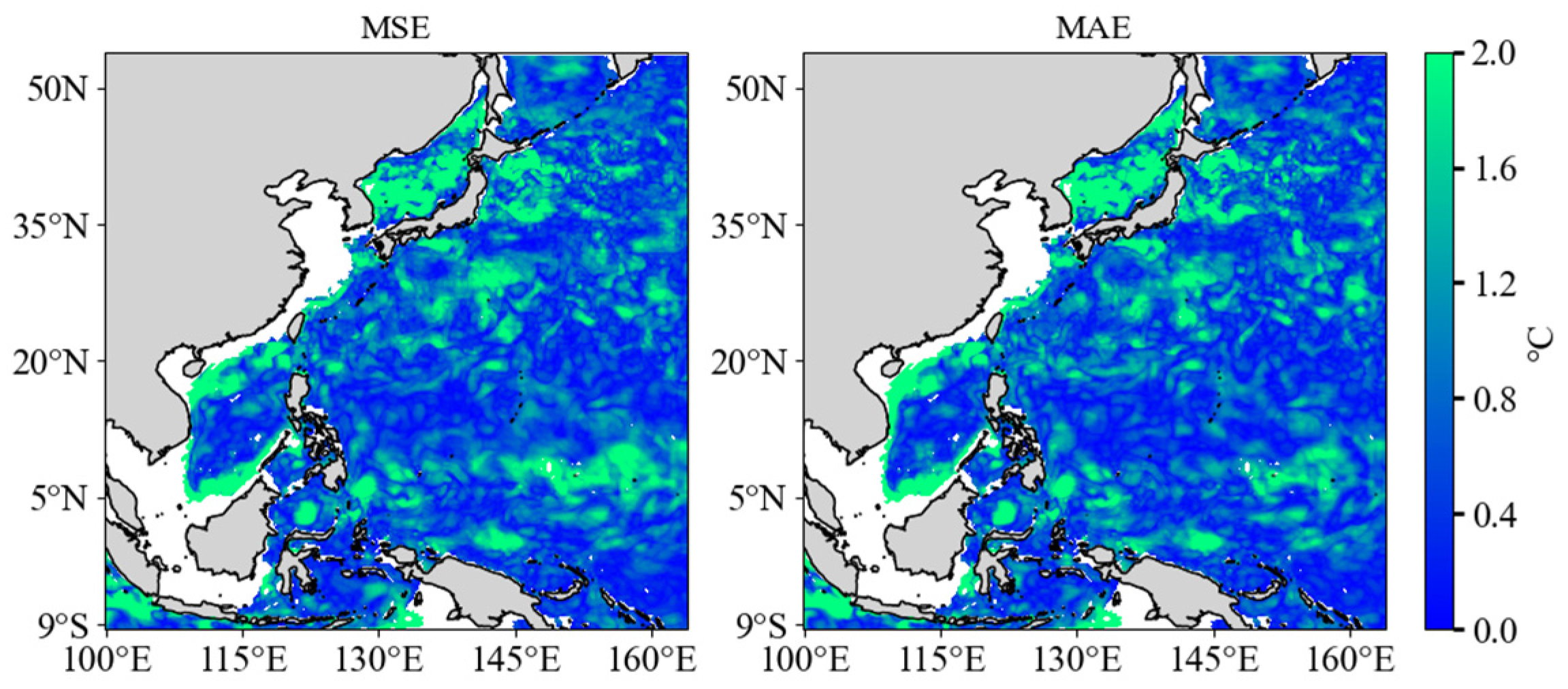
According to Figure 7, the temperature field reconstructed using MSE and MAE loss functions has no significant spatial error and is in good agreement with the reconstructed temperature field distribution. Figure 8 shows the distribution of errors over time. The time distribution of RMSE also indicates that RMSE has different characteristics in different seasons: in summer and autumn, RMSE is generally larger, indicating that reconstruction errors are greater during these periods.

Since the MSE loss function is more sensitive to data anomalies, it can better learn the characteristics of the input data, and the error in the output results is smaller, with a higher correlation to the original data. Therefore, the MSE function is better suited for the reconstruction of three-dimensional temperature fields.

3.3. Verification and Assessment of Temperature Field Inversion in the Northwest Pacific and Offshore China

Next, taking the experimental results of Experiment Group 2 (input variables SSTA, SLA, labeled data STA, and loss function MSE) as the most suitable input–output and loss function for training the model, combined with GLORYS reanalysis data and the reconstruction results of the U-net network, we analyze the accuracy of the temperature field reconstruction in the Northwest Pacific and offshore China.

The overall accuracy of the reconstruction results is calculated by using a scatterplot of temperature distribution. Figure 9 presents the scatterplots of the reconstructed temperature data and the original data distribution in different months, with all points of the reconstructed temperature data and the original data marked in Figure 9. The temperature field reconstructed by the U-net network accurately reflects the temperature distribution, and the distribution of the reconstruction results resemble those of the original data, indicating that the model is trained well.

Figure 10 shows the meridional-depth distribution of the zonal-averaged RMSE. It can be seen that the overall vertical reconstruction results are relatively good, with only some significant errors in certain areas of the upper water body because the upper layer belongs to the thermocline. Due to the fact that the majority of the thermocline range in the study area is between 0 and 300 m, there is a significant error in temperature inversion in the upper layer [33].

To further examine the spatial distribution of the reconstruction, the RMSE distribution of the reconstructed temperature field RMSE at 55 m and 109 m within the 4° × 4° square area for the whole year of 2018 is plotted in Figure 11. From the results, the spatial distribution of RMSE tends to average with the increase of water depth, and the high values of error are mainly distributed in the west-south coast of the South China Sea, the northern part of the East China Sea, and parts of the high latitude region of the Northwest Pacific Ocean, which lead to the large reconstruction error due to the proximity to land and more obvious temperature changes.

3.4. Performance of the Reconstructed Three-Dimensional Temperature Field for Typical Mesoscale Eddies

Oceans have various scales of motion. Large-scale, relatively stable seawater flows are called currents, while the rotational motion of water bodies at the scale of 10–100 km is known as mesoscale eddies. These are a common dynamic phenomenon in oceans, serving as the main carriers of oceanic kinetic energy, and they play an important role in the distribution of oceanic materials and energy. They are also the main source of mesoscale sea temperature variability and trigger mesoscale air–sea interaction processes, which have a shaping effect on large-scale ocean circulation and regional climate.

We can train deep learning models with a large amount of satellite data and then use these models to identify mesoscale eddies. Based on the research structure mentioned earlier, the distribution and characteristics of the eddies in the Northwest Pacific are analyzed using the corresponding reconstructed temperature field data.

Comparing the reconstruction with the original GLORYS data, we observe the eddy performance to verify the accuracy of the model. To further explore the spatial characteristics of the reconstructed eddies, points A (135° E, 30° N) and B (138°E, 32°N) in the reconstructed temperature field are selected to represent the two areas to analyze the vertical temperature distribution of the eddies (Figure 12).

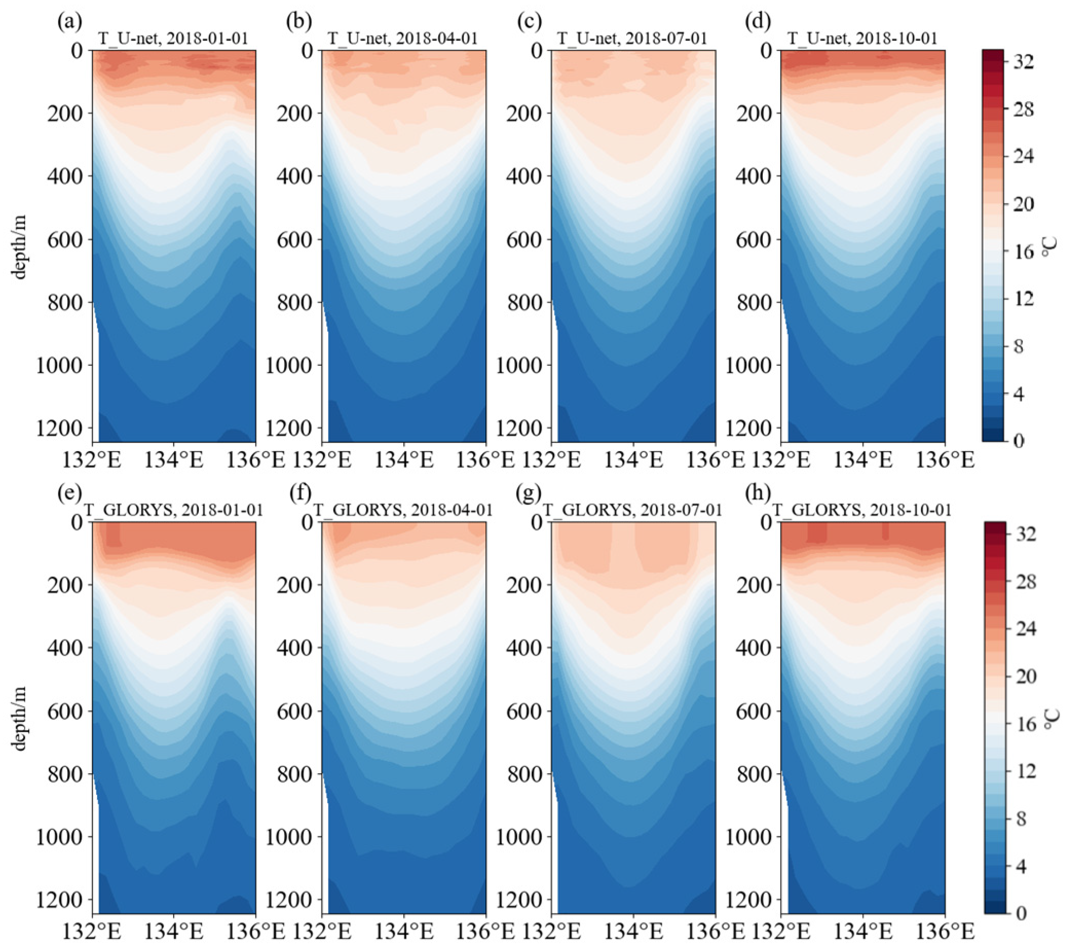
Based on the above, there are rather obvious eddies within the range of (130° E–145° E, 25° N–35° N). Figure 13 and Figure 14 show the vertical distribution of reconstructed and original temperature fields for the eddies at locations A and B, and the U-net network still maintains a high degree of accuracy in reconstructing eddies. The warm eddy at location A does not show significant changes in position across different seasons, and its depth remains essentially unchanged, extending to as deep as 600 m below the surface. In winter and autumn, when the surface temperature is higher, the eddy at location A is more pronounced in the upper layer. Meanwhile, the cold eddy at location B shifts position across different seasons, being more prominent in winter and spring.

Through the analysis of individual eddies in the reconstructed three-dimensional temperature field results, the performance of the reconstructed temperature field in the eddy identification is evaluated, and the reconstructed eddies are shown to be highly consistent with the corresponding ones in the original data at the same location. This indicates that the reconstructed temperature field using the U-net network possesses strong applicability to construct the three-dimensional structure of mesoscale eddies.

4. Discussion and Conclusions

In this study, based on reanalysis data, the underwater three-dimensional temperature structure of the Northwest Pacific and offshore China was reconstructed using the U-net deep learning model with different data formats and loss functions. Through the analysis of the reconstruction results, the most suitable data format and loss function for the reconstruction of the three-dimensional temperature field were determined. The reconstruction results were subjected to validation analysis, and the mesoscale eddies within the reconstructed temperature field were analyzed.

Four control experiments were designed to explore the impact of using normal and anomaly values as input variables on model accuracy and to investigate whether normalized labeled data would affect the reconstruction results. The conclusion reached was that, for the U-net network, inputting anomaly value data compared to the original temperature values can achieve higher accuracy in the reconstruction of the three-dimensional temperature field in the Northwest Pacific. With the input data remaining unchanged, using the normalized temperature anomalies as labels can yield more accurate outcomes.

Next, the impact of setting different loss functions on the reconstruction accuracy of the model was evaluated. Based on the experimental results from the previous section, two sets of experiments were conducted with MSE and MAE set as the model’s loss functions to explore the impact of different loss functions on the reconstruction results. By comparing the experimental outcomes, it was observed that when reconstructing the three-dimensional temperature field, the overall accuracy of the reconstruction results was similar for the two loss functions. In the shallow water areas, the reconstruction results using the MSE loss function were slightly better than those using MAE, while in the deep water areas, there was little difference.

After statistical analysis of the reconstruction error, the reconstruction results of the U-net network showed high consistency with the original temperature field. The distribution of errors showed similar trends in different seasons, but its characteristics differed depending on the depth. Spatially, in areas with significant temperature gradients or temperature anomalies, in the ranges of 35–40° N and 0–10° N, the error is markedly higher than in other study regions. Moreover, the errors are primarily concentrated in the upper ocean layers within 500 m. Next, by analyzing the distribution and characteristics of some mesoscale eddies within the reconstructed temperature field, the accuracy of the U-net network for mesoscale eddy analysis was verified. It was shown that the U-net network can effectively reconstruct the horizontal and vertical features of mesoscale eddies in the temperature field, with the reconstructed mesoscale eddies showing high consistency with the original data, and it is capable of accurately identifying and reconstructing both cold and warm eddies in the Northwest Pacific.

Through this study, a three-dimensional temperature field with a high spatiotemporal resolution was established in the Northwest Pacific Ocean using the U-net network, and mesoscale eddies there were also identified. Although relatively accurate results were obtained, there remain some shortcomings, especially for temperature inversion near 200 m.

When reconstructing the temperature field, only two variables—sea surface temperature and sea surface height—were considered, and there was no attempt to analyze the impact of other sea surface data on temperature field reconstruction. While the current reconstruction accuracy meets certain requirements, adding other sea surface variables in the reconstruction may further improve the reconstruction accuracy.

Only two loss functions with simple structure and wide application—MSE and MAE—were selected for the U-net network, yet other types of loss functions may yield superior outcomes in temperature field reconstruction. If we can find or design loss functions that are more suited for temperature field reconstruction through experiments, or determine superior experimental schemes through experiments, then the accuracy of reconstruction may be further improved.

Finally, this study employed the U-net deep learning model for temperature field reconstruction, using a rather singular approach. Exploring ways to optimize and modify the model to achieve higher output accuracy during reconstruction is a direction worth investigating.