Noise Reduction of Velocity Measured by Frequency-Supervised Combined Doppler Sonar Using an Adaptive Sliding Window and Kalman Filter

Abstract

Velocity is fundamental information for ocean engineering. It is difficult for traditional Doppler sonar to provide accurate and wide-range velocity measurement information with a short time lag. Therefore, a frequency-supervised combined Doppler sonar system using an adaptive sliding window and Kalman filter is proposed. In this method, the initial value of the integer ambiguity is calculated based on the average value of the conventional Doppler sonar. The change value of the integer ambiguity is calculated by the difference of the adjacent velocities measured by coherent Doppler sonar. The velocity of combined Doppler sonar is calculated by the cumulative result of the initial and change values of integer ambiguities. Finally, the velocity bias due to the error of the integer ambiguity calculation is corrected by the frequency supervision using the Kalman filter in a sliding time window under different signal-to-noise ratios. The experimental results show that the proposed method is more accurate than the conventional Doppler sonar, has a wider measurement range compared with coherent Doppler sonar, and suppresses the impulsive noise well. The frequency-supervised combined Doppler sonar using an adaptive sliding window and Kalman filter can provide accurate and precise velocities with a short time lag over a wide range of signal-to-noise ratios.

1. Introduction

For ships and undersea vehicles, velocity is an essential component of information that is also crucial to navigation and ocean engineering. Conventional Doppler sonar (CNDS) has been widely used to provide speed information as a basic device installed on vessels. However, ambient noise and ship noise (where the equipment is installed) can affect velocity measurements. At low signal-to-noise ratios (SNRs), CNDS provides valuable velocity readings with a time lag lasting for seconds [1], which is insufficient for tasks requiring high velocity accuracy. Pulse-to-pulse coherent Doppler sonar (CHDS) was created to investigate fluid characteristics in the ocean, such as turbulence and wave characteristics [2,3]. Velocities measured by CHDS are accurate with minimal time lag [4,5], but the presence of “range-velocity” ambiguities has limited the wider application of CHDS. To increase the maximum measurable velocity, multiple pulse repetition frequencies [6,7] and carrier frequencies [8,9] have been used, but the results are still unsatisfactory.

A combined method using Doppler shift and phase shift (CMDS) [10,11] has been proposed to compute velocity information. CMDS computes velocities as accurately as CHDS and without velocity ambiguity. However, CMDS generates impulsive noise due to the misestimation of the integer ambiguity. The Kalman filter is utilized to estimate the state of a dynamic system based on a series of noisy measurements, with noise reduction being its primary application [12,13]. To decrease the probability of wrong estimation of the integer ambiguity, the Kalman filter and linear prediction (CMDS_KL) were introduced [14]. The method decreased the impulsive noise significantly, but it was sensitive to the initial value and might not perform well for non-smooth processes containing abrupt or sudden changes.

To overcome the shortcomings of CMDS_KL, a frequency-supervised CMDS using an adaptive sliding window and Kalman filter (CMDS_FK) was proposed. Section 2 will introduce the basic concepts of CNDS, CHDS, and CMDS. Then the data processing of velocity measured by CMDS_FK is introduced. In Section 3, the experimentation with velocity measured by the proposed method is described. Section 4 shows the experiment results and comparisons of CHDS, CNDS, CMDS, CMDS_KL, CMDS_FK, and CMDS filtered by median and mean filters. The conclusion is found in Section 5.

2. Methods

2.1. Conventional Doppler Sonar (CNDS)

CNDS was created to measure the speed of ships and submarines using the Doppler effect. As determined by the CNDS beam, the radial Doppler frequency shift [15,16] is

$$f_D=f_{rx}-f_{tx}=f_{tx}\left({\displaystyle \frac{1\pm \frac{v_r}{c}}{1\mp \frac{v_r}{c}}}\right)-f_{tx}\approx \pm {\displaystyle \frac{2v_r}{c}}{f}_{tx}$$

(1)

where

$f_{rx}$ is the received frequency;

$f_{tx}$ is the transmitted frequency;

$v_r$ is the radial velocity of the ship in the beam direction;

$c$ is the speed of sound.

Based on Equation (1), velocity can be measured without ambiguity. However, CNDS cannot provide precise velocity at low SNR. In order to improve the precision of velocity, CNDS used a smoothing operation, which requires a few seconds of time lag, to provide valuable readings of velocity [1].

2.2. Coherent Doppler Sonar (CHDS)

By calculating the phase difference of successively received signals, the velocity of CHDS is determined. It is normally used to measure currents and turbulence [17]. In the situation that hydrophones and transducers are located on the same side of the neighborhood, the velocity of CHDS can be calculated as shown below [18]:

$$v={\displaystyle \frac{\phi c}{4\pi f_c\tau }},$$

(2)

where

$\phi$ is the phase change of the adjacent received signals, limited from −$\pi$ to $\pi$;

$c$ is the speed of sound in water;

$\tau$ is the time interval between adjacent pulses;

$f_c$ is the carrier frequency.

The accurate velocity determined by CHDS has a short latency. However, the ambiguity velocity ($\Delta v$) is obtained while $\phi =\pi$, and the maximum space range ($\Delta R$) is achieved as $\Delta R=c\tau /2$. Then, the ‘range-velocity’ ambiguity can be expressed as

$$\Delta R \Delta v={\displaystyle \frac{c\lambda }{8}} ,$$

(3)

where $\lambda$ is the wave length of the system, that is $\lambda =c/f_c$. In a determined sonar system, $c$ and $\lambda$ are known determinants. Therefore, $\Delta v$ is inversely proportional to $\Delta R$, limiting more general applications of CHDS.

If the radial velocity $v$ is greater than $\Delta v$, the true velocity $v$ can be expressed as

$$v=2n\Delta v+v_h,$$

(4)

where $v_h$ is the velocity measured by CHDS and $n$ the integer ambiguity. Using the velocity determined by CMDS, the value of integer ambiguity $n$ is found.

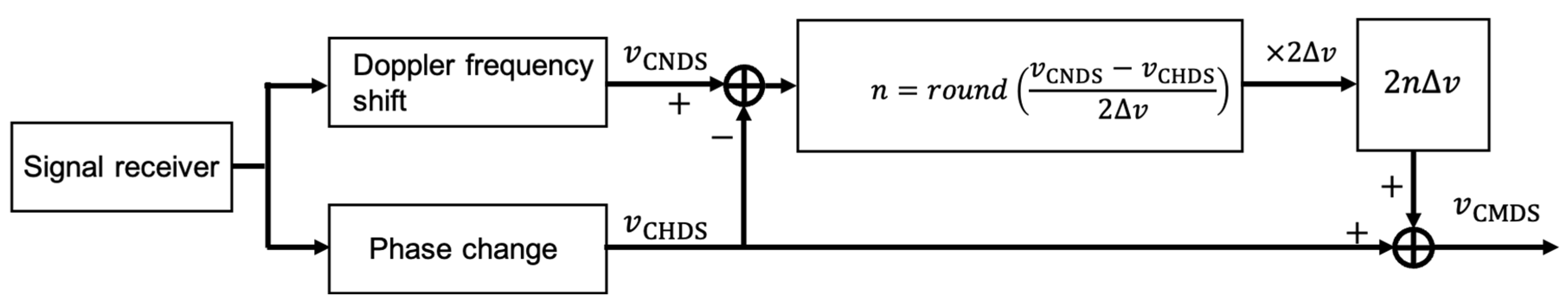
2.3. Combined Doppler Sonar (CMDS)

Figure 1 illustrates the CMDS velocity measurement procedure. Each pair of broadcasted and received signals can be used to calculate velocity using the CNDS ($v_{\mathrm{CNDS}}$). With CHDS ($v_{\mathrm{CHDS}}$), the velocity can also be calculated by observing the phase difference between two nearby received signals. Then the integer ambiguity $n$ can be calculated as

$$n=round\left({\displaystyle \frac{v_{\mathrm{CNDS}}-v_{\mathrm{CHDS}}}{2\Delta v}}\right)$$

(5)

where

$v_{\mathrm{CNDS}}$ is the velocity measured by CNDS according to Equation (1);

$v_{\mathrm{CHDS}}$ is the velocity measured by CHDS according to Equation (2);

$round\left(\cdot \right)$ is the function to calculate the nearest integer value.

Figure 1. CMDS-measured velocity process.

Figure 1. CMDS-measured velocity process.

Based on Equation (5), the accuracy of the integer ambiguity $n$ is determined by the measurement errors of CNDS and CHDS. When the integer ambiguity n was determined correctly, CMDS could provide velocities as accurate as CHDS without range limitation. In low SNR, the measurement error of CNDS seriously affects the integer ambiguity $n$. Therefore, a new data processing method is proposed to decrease the wrong estimation of integer ambiguity.

2.4. Combined Doppler Sonar Using Kalman Filter and Linear Prediction (CMDS_KL)

Figure 2 shows the CMDS_KL velocity measurement procedure. Velocity measured by CNDS is denoised by the Kalman filter. In the Kalman filter, the state $x$ of a discrete-time controlled process and the measurement $z$ can be expressed as

$$x_{k+1}=A_k{x}_k+B{u}_k+w_k,$$

(6)

$$z_k=H_k{x}_k+l_k,$$

(7)

where

$u$ is the input;

$A$ is the matrix relating the state at time step $k$ to $k$ + 1;

$B$ is the matrix relating the control input $u$ to the state $x$;

$w$ is the process noise;

$H$ is the matrix relating the state $x$ to the measurement $z$;

$l$ is the measurement noise.

Figure 2. CMDS_KL-measured velocity process.

Figure 2. CMDS_KL-measured velocity process.

The denoised $v_{\mathrm{CNDS}}$ by Kalman filter still may generate a wrong estimation of integer ambiguity. Hence, linear prediction [19] is used, and the prediction of the $N$th measured velocity of combined Doppler sonar $v_{\mathrm{CMDS}}$ can be expressed as

$$v_{\mathrm{CMDS}\_\mathrm{L}}\left(N\right)={\displaystyle \sum }_{i=1}^M{h}_i\left(N\right)v_{\mathrm{CMDS}}\left(N-i\right),$$

(8)

where

$v_{\mathrm{CMDS} \mathrm{L}}$ is the predicted velocity;

$M$ is the number of taps;

$h_i$ is the prediction coefficient.

If the predicted velocity is significantly different from the measured velocity, a modified velocity will be obtained, which is

$$v_{\mathrm{CMDS}\_\mathrm{KL}}=v_{\mathrm{CMDS}}-2n_e\Delta v.$$

(9)

where

$$n_e=round\left({\displaystyle \frac{v_{\mathrm{CMDS}}-v_{\mathrm{CMDS}\_\mathrm{L}}}{2\Delta v}}\right).$$

(10)

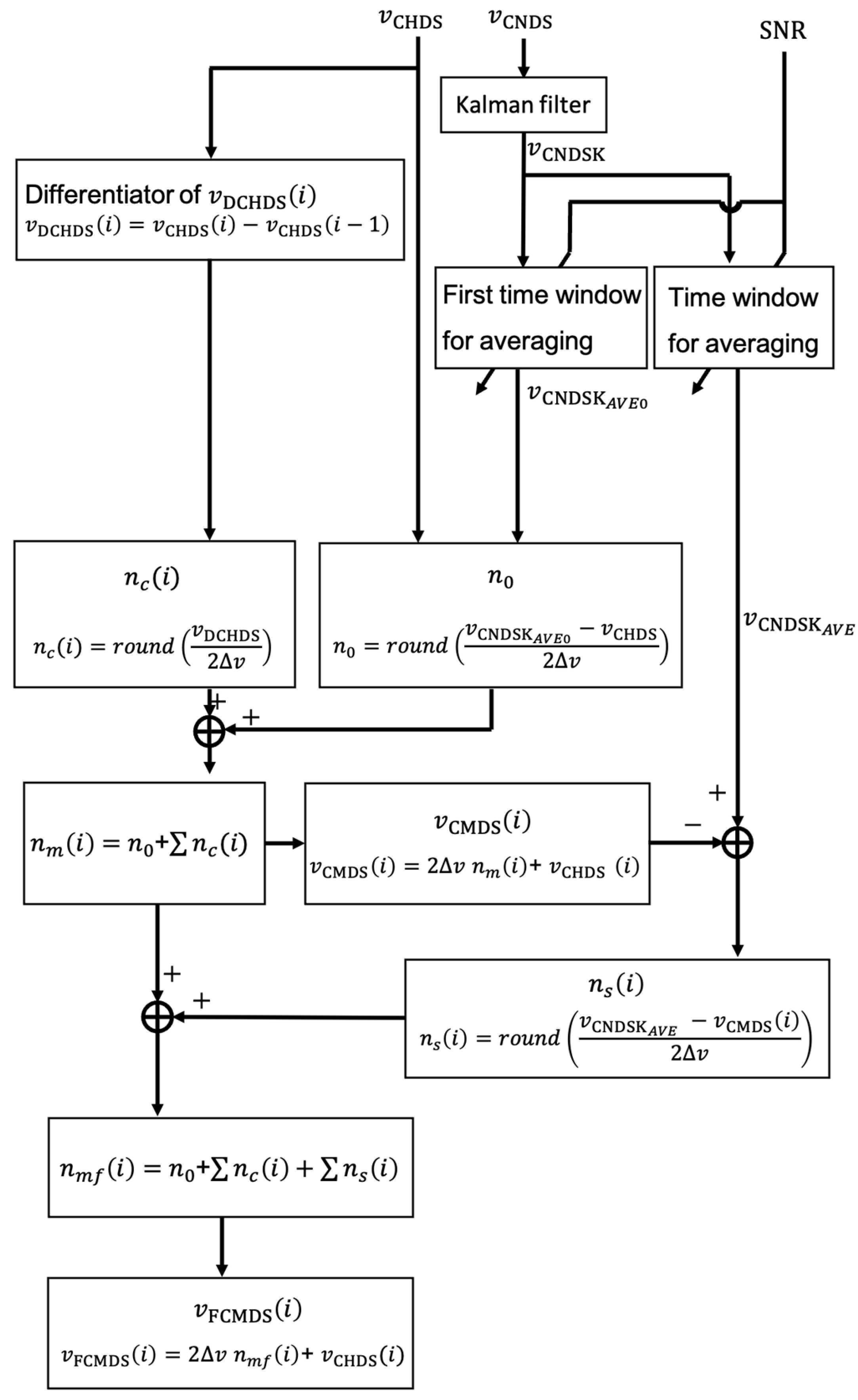
2.5. Frequency-Supervised Combined Doppler Sonar Using an Adaptive Sliding Window and Kalman Filter (CMDS_FK)

Figure 3 shows the CMDS_FK velocity measurement procedure. In the CMDS_FK model, the velocity measured by CNDS is filtered by the Kalman filter ($v_{\mathrm{CNDSK}}$) to decrease the measurement noise. The Kalman filter [20] has been widely used in ocean engineering [21,22,23], which can be used to suppress noise. Then, an initial velocity of CNDS used for the integer ambiguity estimation ($v_{{\mathrm{CNDSK}}_{AVE0}}$) is obtained from the average value in a time window. The length of the time window is the same as used to reduce the bias, and the adaptive average number $M$ at the SNR is proposed as

$$M>{\displaystyle \frac{9{{\sigma }_f}^2}{\Delta v}},$$

(11)

where ${\sigma }_f$ is the standard deviation of velocity measured by CNDS by employing the Kalman filter at the SNR. The measurement error of CHDS is much less than CNDS [1], and the measurement error of ($v_{\mathrm{CNDSK}}-v_{\mathrm{CHDS}}$) is approximate to the error of $v_{\mathrm{CNDSK}}$. Using the adaptive average number $M$, ${\sigma }_f$ is decreased to be less than $\Delta v/3$. According to Equation (5), the probability of the wrong estimation of the integer ambiguity is decreased by approximately 99% based on Gaussian distribution. Compared with a small fixed window, the adaptive window for averaging could provide a more accurate estimation result of the integer ambiguity in low SNR. Compared with a large fixed window, the adaptive method needs a small averaging time in high SNR.

Based on Equation (5), the initial integer ambiguity can be obtained as

$$n_0=round\left({\displaystyle \frac{v_{{\mathrm{CNDSK}}_{AVE0}}-v_{\mathrm{CHDS}}\left(0\right)}{2\Delta v}}\right),$$

(12)

where $v_{\mathrm{CHDS}}\left(0\right)$ is the first measured velocity of CHDS.

Although CHDS measures velocity precisely, there is some velocity ambiguity. In the situation where the measured velocity is greater than the ambiguity velocity $\Delta v$, the measured velocity of CHDS cannot be used directly. Therefore, in CMDS_FK, the differential result of two consecutive velocities is used. Assuming that the acceleration of the moving object under test is less than $\Delta v/\tau$, the velocity change significantly occurs when the value of integer ambiguity $n$ changes. The change value $n_c$ can be expressed as

$$n_c\left(i\right)=round\left({\displaystyle \frac{v_{\mathrm{DCHDS}}\left(i\right)}{2\Delta v}}\right),$$

(13)

where

$$v_{\mathrm{DCHDS}}\left(i\right)=v_{\mathrm{CHDS}}\left(i\right)-v_{\mathrm{CHDS}}\left(i-1\right), i=1,2,3\dots$$

(14)

Based on the initial and change values of integer ambiguity, the velocity of CMDS can be calculated as

$$v_{\mathrm{CMDS}}\left(i\right)=2\Delta v\left(\sum n_c\left(i\right)+n_0\right)+v_{\mathrm{CHDS}}\left(i\right)$$

(15)

In this calculation, the value of $n_c$ is limited by three values, −1, 0, and 1. In the situation of a large acceleration of the detected object or accidental wrong measurements of CHDS, $n_c$ cannot be calculated correctly. If the wrong value of $n_c$ exists, a subsequent velocity bias will occur due to the accumulation in Equation (15).

To reduce the bias, the average of measured velocities by CNDS in a sliding time window $v_{{\mathrm{CNDSK}}_{AVE}}$ is used as a supervisor. To make the detection of integer ambiguity bias correctly, the average number $M$ is used based on Equation (11). If the difference between $v_{\mathrm{CMDS}}\left(i\right)$ and $v_{{\mathrm{CNDSK}}_{AVE}}$ is large, the bias generated by the wrong calculation of $n_c$ may exist. The bias of the estimated integer ambiguity can be calculated as

$$n_s\left(i\right)=round\left({\displaystyle \frac{v_{{\mathrm{CNDSK}}_{AVE}}-v_{\mathrm{CMDS}}\left(i\right)}{2\Delta v}}\right).$$

(16)

Then, the modified integer ambiguity is obtained as follows:

$$n_{mf}\left(i\right)=n_0+\sum n_c\left(i\right)+\sum n_s\left(i\right)$$

(17)

Finally, the velocity measured by CMDS_FK can be obtained as

$$v_{\mathrm{CMDS}\_\mathrm{FK}}\left(i\right)=2n_{mf}\left(i\right)\Delta v+v_{\mathrm{CHDS}}\left(i\right)$$

(18)

In this model, the initial value of integer ambiguity is determined by the initial average of CNDS and initial CHDS, the change value of integer ambiguity is calculated from the change results of CHDS, and the bias value of integer ambiguity is corrected by the sliding average of CNDS. Therefore, the velocity measured by CMDS_FK, which takes advantage of CHDS and averaged CNDS, could deliver precise and accurate velocity without ambiguity about velocity.

3. Error Analysis

Based on Equation (18), the measurement error of CMDS_FK is derived from the wrong estimation of the integer ambiguity $n_{mf}$ and the measured velocity error of CHDS. Suppose the measured velocity errors of CNDS and CHDS follow the Gaussian distribution, then the measurement error of velocity measured by CMDS_FK can be obtained as

$${\sigma }_{mf}=\sqrt{{{\sigma }_h}^2+{\displaystyle \sum }_{n_{mfe}\in Z}P(n_{mfe}){\left(2n_{mfe}\Delta v\right)}^2}.$$

(19)

where

${\sigma }_h$ is the standard deviation of velocity measured by CHDS;

$n_{mfe}$ is the estimated integer error of the integer ambiguity $n_{mf}$;

$P(n_{mfe})$ is the probability density of $n_{mfe}$ occurring.

According to Equation (17), the integer ambiguity $n_{mf}$ is made up of three parts, $n_0$, $n_c$, and $n_s$. $n_0$ is calculated by the average value of CNDS in the time window, which is accurate compared with the situation using a single velocity. $n_c$ is obtained by the difference in adjacent velocity measured by CHDS. CHDS is accurate, and the wrong estimation of $n_c$ is infrequent. $n_s$ is estimated by the average value of CNDS using a sliding time window, proposed as supervision for the measurement of CMDS to modify the wrong estimation generated by $n_0$ and $n_c$. To summarize, the integer ambiguity in the CMDS_FK has a low probability of being the wrong estimation. The average of CNDS is used to generate an initial value and supervise the measurement in the CMDS_FK, which means that the velocity measured by the CMDS_FK is not affected by the time lag created by the average.

4. Experiments

The system structure depicted in Figure 4 served as the basis for conducting the experiment. The waveform generator WF1973 (NF Corporation, Yokohama, Japan) produces a square pulse. The square pulse is amplified by the amplifier HAS4011 (NF Corporation, Yokohama, Japan). The amplified square pulse is transmitted by the transducer TC2111 (Teledyne RESON Inc., New York, NY, USA). The pulse propagates in a water tank with size of 150 cm × 70 cm × 70 cm. The transmitted pulse signal is received by the hydrophone TC4034 (Teledyne RESON Inc., New York, NY, USA). Then, the received signal of the hydrophone is amplified by the amplifier 5307 (NF Corporation, Yokohama, Japan). The acquisition card NI Pxie-5122 (National Instruments Co., Tokyo, Japan (Branch Office)) samples both the pulse signal that is broadcasted and the amplified signal that is received. In the experiment, the transducer is moved by the 3D moving device Super FA (THK Co., Tokyo, Japan), and the trajectory of the transducer is reciprocating towards the hydrophone.

Table 1. Equipment parameters.

Parameters	Values
Pulse Envelop	Square
Length of Pulse	0.6 ms
Size of Water Tank	150 cm × 70 cm × 70 cm
Accuracy of Moving Machine	1 mm/s
Carrier Frequency of Pulse	200 kHz
Pulse Repetition Frequency	50 Hz
Stable Moving Velocity of Transducer	0.300 m/s
Depth of the Hydrophone and the Transducer	0.20 m
Temperature	10.8 °C
Sound Speed	1450 m/s

displays the parameters that were used in the experiment. Different SNRs are achieved by turning the ambiguity of the transmitted signal generated by the waveform generator WF1973.

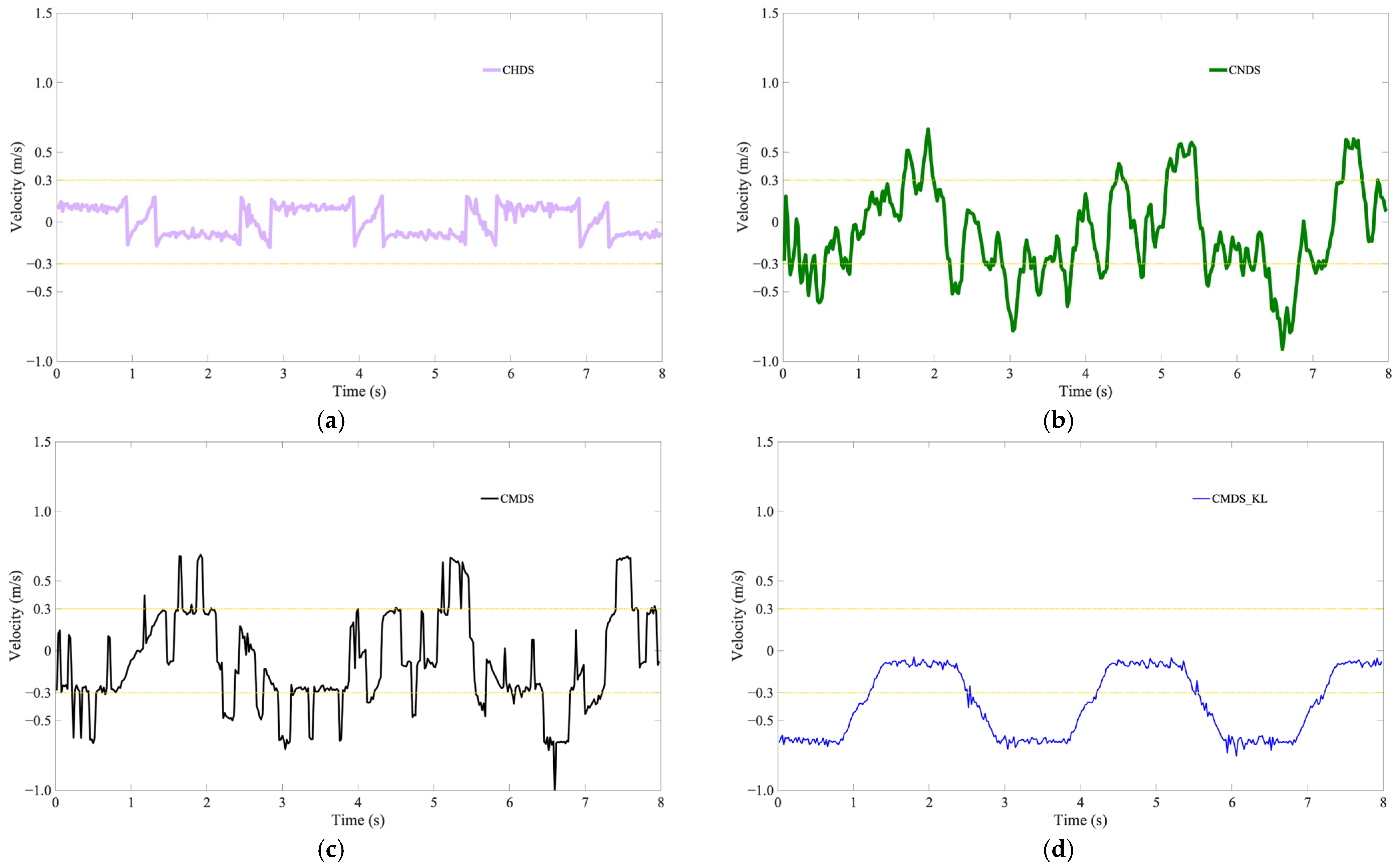
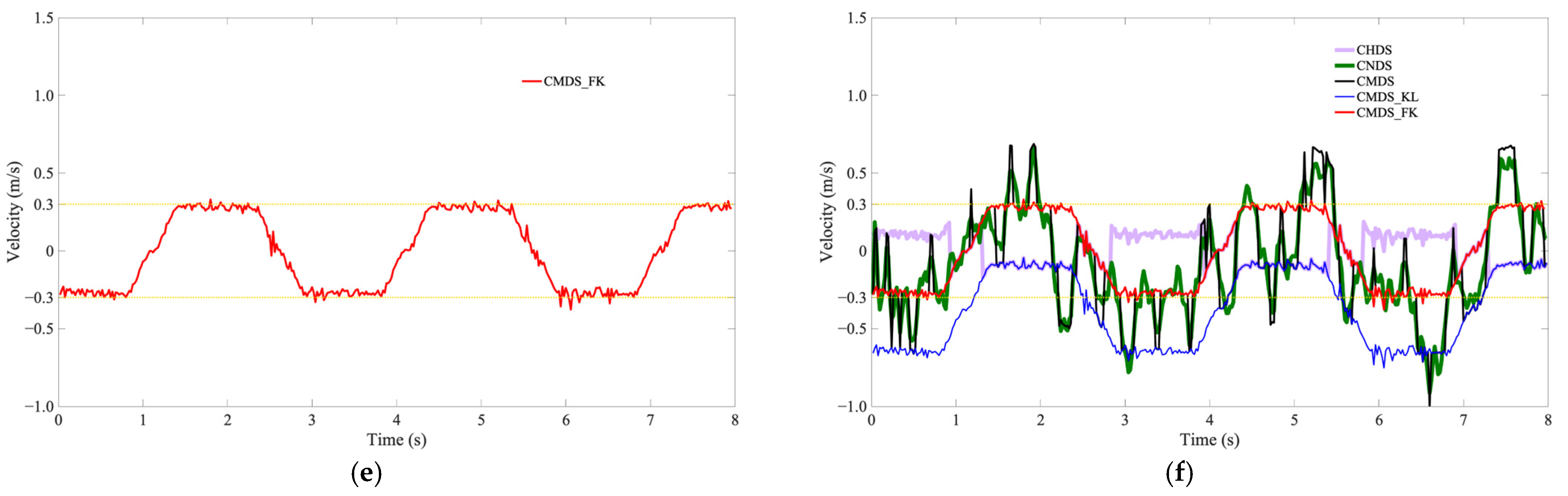
5. Results and Discussion

Based on the system structure, the hydrophone and the transducer are separate, resulting in twice the ambiguity velocity by Equation (4). Therefore, given the pulse interval and the carrier frequency, the ambiguity velocity of CHDS is 0.181 m/s, which is below the stable moving velocity of the transducer. In this situation, an integer ambiguity occurs. The measured velocities of CHDS, CNDS, CMDS, CMDS_KL, and CMDS_FK are laid out in Figure 5. The parameters used in the Kalman filter are manually turned. The standard deviation of the filtered velocity is used as an evaluation index for Kalman filter parameters. The final used parameters are shown in

Table 2. Parameters of the Kalman filter.

Parameters	Values
State Transition Matrix	$\left[\begin{array}{cc}1& 0.1\\ 0& 1\end{array}\right]$
Control Input Matrix	$\left[\begin{array}{c}0.005\\ 0.1\end{array}\right]$
Measurement Matrix	$\left[\begin{array}{cc}1& 0\end{array}\right]$
Covariance of Observation Noise	$\mathrm{Deviation} \mathrm{of} v_{CNDS}$
Covariance of Process Noise	0.06

. In Figure 5, the SNR is −11.1 dB. The velocities measured by CHDS are shown in Figure 5a, which are precise but contain the wrong measurement when the moving velocity is larger than the ambiguity velocity. Figure 5b shows the velocities measured by CNDS, which are noisy. Figure 5c shows the velocities measured by CMDS, which are generally accurate but contain a lot of impulsive noise because of the integer ambiguity. Figure 5d shows the velocities measured by CMDS_KL, which are precise and without impulsive noise. However, with the wrong estimation of the initial value in the Kalman filter, there is an overall bias in the measured velocities. In Figure 5e, the velocity measured by CMDS_FK is accurate, without ambiguity velocity, impulsive noise, or velocity bias. Compared with Figure 5e, only a velocity bias exists in the Figure 5d.

Figure 6 shows the velocities measured by five methods at an SNR of 15.4 dB. In Figure 6a, CHDS provides precise velocity but contains velocity ambiguity, and some impulsive noise occurs when the measured velocity is near the value of ambiguity velocity. In the high SNR, the velocities measured by CNDS in Figure 6b are much better than those in the low SNR but cannot be as accurate as CMDS in Figure 6c. In Figure 6d, the velocities measured by CMDS_KL contain a bias generated by the impulsive noise of CHDS. The velocities measured by CMDS_FK modify the velocity bias shown in Figure 6e, but the proposed method cannot eliminate the peaks generated by the velocity measured by CHDS. Based on Figure 5 and Figure 6, CMDS_FK can provide accurate velocity information.

To assess the performance of CMDS_FK, a median filter and a mean filter are used to carry out the comparison. The median filter can be used to suppress impulsive noise [24]. In sonar systems, the mean filter is typically employed to increase the precision of the observed velocity. The filtered results of the velocities measured by CMDS using filters at an SNR of −11.1 dB are shown in Figure 7. The filtered results of CMDS by median filter with 0.5 s are shown as the blue line, and the mean filter with 0.5 s is in the pink line. While going smoothly and with minimal impulsive noise, the median filter works well. However, while moving at a changing speed or when the measured velocity of the CMDS fluctuates due to an incorrect estimate of the integer ambiguity, it produces a considerable bias. The impulsive noise is eliminated by the mean filter, but detailed moving information is lost, and the accuracy is worse than CMDS_FK, as seen by the red line.

An average value of velocity measured in the stable moving process is shown in Figure 8. The average value is calculated in 4 s. As shown in Figure 8, the average velocity of CMDS_FK is closer to the true value compared with CMDS and CMDS using median and mean filters in the SNR of −11.1 dB. When the SNR is greater than −5 dB, the average values of measured velocity by CMDS, CMDS using median filter, and CMDS_FK are similar.

The standard deviations (STDs) of measured velocity by the four methods are shown in Figure 9. The STD is calculated while the transducer moves with a stable velocity. As shown in Figure 9, the STDs of CMDS using median and mean filters decreased significantly. In the situation where the SNR is greater than 0 dB, the STD of CMDS_FK is similar to that of the CMDS using the median filter and much better than that of the CMDS and the CMDS using the mean filter. When the SNR is less than 0 dB, the STD of CMDS_FK is smaller than the other three methods, especially in the situation where the SNR is less than −5 dB. Thus, over a wide range of SNR, CMDS_FK can offer a minimal measurement error.

6. Conclusions

CMDS is a method that takes advantage of CHDS with precise velocity measurement and CNDS without velocity ambiguity. However, the impulsive noise occurs when the integer ambiguity is falsely estimated. To lessen impulsive noise, CMDS added the Kalman filter and linear prediction; nevertheless, this was impacted by the observed velocity’s beginning value and an incorrect CHDS computation. As a result, it is suggested that CMDS_FK offers accurate velocity over a wide SNR range. In this method, first, an average of velocities measured by CNDS in the time window determined by the SNR is used to estimate the reasonable initial value for the first integer ambiguity calculation. Then, the change in integer ambiguity is calculated by the difference of adjacent velocities measured by CHDS. Finally, the CMDS velocity value is calculated by combining the cumulative result of the integer ambiguity changes with the CHDS velocity. The average of the velocities detected by CNDS employing the Kalman filter in the sliding time window set by the SNR is employed to eliminate the velocity bias caused by the incorrect estimation of integer ambiguity changes.

A comparison of CHDS, CNDS, CMDS, CMDS_KL, and CMDS_FK was presented. CMDS_FK could provide accurate velocity without ambiguity velocity and is unaffected by the anomalies of velocity measured by CHDS. Additionally, mean and median filters were included in order to assess CMDS_FK’s performance. The findings demonstrate that, throughout a wide range of SNR, the velocity measured by the suggested approach had minimal standard deviations with a short time latency. As a result, CMDS_FK can considerably reduce impulsive noise and offer precise velocity with a low latency, which may be advantageous for docking, navigation, and operating underwater vehicles and marine engineering.

In the present study, the experiments in the laboratory verified the feasibility and validity of CMDS_FK. Therefore, the reliability and measurement accuracy of the proposed method in the presence of a large number of reflected signals and complex environmental noise should be evaluated in the next step.

Reducing the impulsive noise of CMDS is a work of fault diagnosis. Machine learning theories, especially deep learning theories, have been proven to be an efficient tool for dealing with fault diagnosis [25]. In future work, machine learning theories will be introduced in the CMDS systems to reduce the impulsive noise generated by the wrong estimation of the integer ambiguity.

References

1. Doisy, Y. Theoretical Accuracy of Doppler Navigation Sonars and Acoustic Doppler Current Profilers. IEEE J. Ocean. Eng. 2004, 29, 430–441. [Google Scholar] [CrossRef]
2. Lohrmann, A.; Hackett, B.; Roed, L.P. High resolution measurements of turbulence, velocity and stress using a pulse-to-pulse coherent sonar. J. Atmos. Ocean Technol. 1990, 7, 19–37. [Google Scholar] [CrossRef]
3. Veron, F.; Melville, W.K. Pulse-to-pulse coherent Doppler measurements of waves and turbulence. J. Atmos. Ocean Technol. 1999, 16, 1580–1597. [Google Scholar] [CrossRef]
4. Lhermitte, R.; Serafin, R. Pulse-to-pulse coherent Doppler sonar signal processing techniques. J. Atmos. Ocean Technol. 1984, 1, 293–308. [Google Scholar] [CrossRef]
5. Zedel, L. Modeling pulse-to-pulse coherent Doppler sonar. J. Atmos. Ocean Technol. 2008, 25, 1834–1844. [Google Scholar] [CrossRef]
6. Holleman, I.; Beekhuis, H. Analysis and correction of dual PRF velocity data. J. Atmos. Ocean Technol. 2003, 20, 443–453. [Google Scholar] [CrossRef]
7. Joe, P.; May, P.T. Correction of dual PRF velocity errors for operational Doppler weather radars. J. Atmos. Ocean Technol. 2003, 20, 429–442. [Google Scholar] [CrossRef]
8. Hay, A.E.; Zedel, L.; Craig, R.; Paul, W. Multi-frequency, pulse-to-pulse coherent Doppler sonar profiler. In Proceedings of the 9th IEEE/OES/CMTC Working Conference on Current Measurement Technology, Charleston, SC, USA, 17–19 March 2008. [Google Scholar]
9. Zedel, L.; Hay, A.E. Resolving velocity ambiguity in multifrequency, pulse-to-pulse coherent Doppler sonar. IEEE J. Ocean. Eng. 2010, 35, 847–851. [Google Scholar] [CrossRef]
10. Liu, P.; Kouguchi, N. Combined Method of Conventional and Coherent Doppler Sonar to Avoid Velocity Ambiguity. J. Mar. Acoust. Soc. Jpn. 2014, 41, 103–112. [Google Scholar] [CrossRef]
11. Liu, P.; Kouguchi, N. Measurement Error Analysis of Combined Doppler Sonar Using Adaptive Algorithm. J. Mar. Acoust. Soc. Jpn. 2015, 42, 11–22. [Google Scholar] [CrossRef]
12. Talebi, S.P.; Godsill, S.J.; Mandic, D.P. Filtering Structures for α-Stable Systems. IEEE Contr. Syst. Lett. 2023, 7, 553–558. [Google Scholar] [CrossRef]
13. Li, C.; Huang, R.; Yi, Y.; Bermak, A. Investigation of filtering algorithm for noise reduction in displacement sensing signal. IEEE Sens. J. 2021, 21, 7808–7812. [Google Scholar] [CrossRef]
14. Liu, P.; Kouguchi, N.; Li, Y. Velocity Measurement of Coherent Doppler Sonar Assisted by Frequency Shift, Kalman Filter and Linear Prediction. J. Mar. Sci. Eng. 2021, 9, 109. [Google Scholar] [CrossRef]
15. Brokloff, N.A. Matrix algorithm for Doppler sonar navigation. In Proceedings of the IEEE OCEANS’94, Brest, France, 13–16 September 1994. [Google Scholar]
16. Taudien, J.Y.; Bilen, S.G. Quantifying Long-Term Accuracy of Sonar Doppler Velocity Logs. IEEE J. Ocean. Eng. 2017, 43, 764–776. [Google Scholar] [CrossRef]
17. Hurther, D.; Lemmin, U.A. A correction method for turbulence measurements with a 3D acoustic Doppler velocity profiler. J. Atmos. Ocean Technol. 2001, 18, 446–458. [Google Scholar] [CrossRef]
18. Dillon, J.; Zedel, L.; Hay, A.E. On the Distribution of Velocity Measurements from Pulse-to-Pulse Coherent Doppler Sonar. IEEE J. Ocean. Eng. 2012, 37, 613–625. [Google Scholar] [CrossRef]
19. Arata, K.; Kensaku, F.; Yoshio, I.; Yutaka, F. A noise reduction method based on linear prediction analysis. Electr. Commun. Jpn. 2003, 86, 1–10. [Google Scholar]
20. Kalman, R.E. A New Approach to Linear Filtering and Prediction Problems. Trans. ASME J. Basic Eng. 1960, 82, 35–45. [Google Scholar] [CrossRef]
21. Shi, Y.; Fang, H.; Yan, M. Kalman filter-based adaptive control for networked systems with unknown parameters and randomly missing outputs. Int. J. Robust Nonlin. 2010, 19, 1976–1992. [Google Scholar] [CrossRef]
22. Thomas, S.; Hofmann, W.; Werner, R. Improving operational performance of active magnetic bearings using Kalman filter and state feedback control. IEEE T. Ind. Electron. 2011, 59, 821–829. [Google Scholar]
23. Lefferts, E.J.; Markley, F.L.; Shuster, M.D. Kalman filtering for spacecraft attitude estimation. J. Guid. Control Dynam. 1982, 5, 417–429. [Google Scholar] [CrossRef]
24. Ravi Kishore, T.; Deergha Rao, K. Efficient median filter for restoration of image and video sequences corrupted by impulsive noise. IETE J. Res. 2010, 56, 219–226. [Google Scholar] [CrossRef]
25. Vashishtha, G.; Chauhan, S.; Sehri, M.; Zimroz, R.; Dumond, P.; Kumar, R.; Gupta, M.K. A roadmap to fault diagnosis of industrial machines via machine learning: Abrief review. Measurement 2025, 242, 116216. [Google Scholar] [CrossRef]
Figure 3. The process of velocity measured by CMDS_FK.
Jmse 12 02320 g003
Figure 4. Experiment system structure. (a) Experimental devices; (b) trajectory of the transducer movement; (c) schematic of velocity change.
Jmse 12 02320 g004
Figure 5. Velocity measured by five different approaches at the speed of 0.300 m/s at an SNR of −11.1 dB: (a) CHDS; (b) CNDS; (c) CMDS; (d) CMDS_KL; (e) CMDS_FK; (f) comparison of velocities measured by five different methods.
Jmse 12 02320 g005aJmse 12 02320 g005b
Figure 6. Velocity measured by five different approaches at the speed of 0.300 m/s (yellow dashed line) at an SNR of 15.4 dB: (a) CHDS; (b) CNDS; (c) CMDS; (d) CMDS_KL; (e) CMDS_FK; (f) comparison of velocities measured by five different methods.
Jmse 12 02320 g006aJmse 12 02320 g006b
Figure 7. Velocity measured by CMDS, CMDS using media and mean filters, and CMDS_FK.
Jmse 12 02320 g007
Figure 8. Average value of velocity measured by CMDS, CMDS using median and mean filters, and CMDS_FK.
Jmse 12 02320 g008
Figure 9. Standard deviation of velocity measured by CMDS, CMDS using median and mean filters, and CMDS_FK.
Jmse 12 02320 g009