3.1. Numerical Method Description
In this study, the fish–water mixtures are regarded as a viscous incompressible continuous liquid phase, and the air is regarded as a viscous compressible continuous gas phase. The three-dimensional unsteady Reynolds-averaged Navier–Stokes equations are as follows:
where
t is time.
p is fluid pressure.
ui and
uj are velocity components.
xi and
xj are displacement components.
μ is the dynamic viscosity coefficient.
ρ is the fluid density.
μt is the turbulent viscosity coefficient.
Due to the complex flow problems, such as large strain rate, swirling flow, and liquid–solid separation in the process of fish suction, the turbulence model adopts SST
k-
ω turbulence model [
18,
19]. The
k-equation and ω-equation of SST
k-
ω are as follows:
where
k is the turbulent kinetic energy,
ω is the turbulent frequency, Γ
k and Γ
ω are the turbulent diffusion coefficients,
Gk and
Gω are the turbulent generation terms,
Yk and
Yω are the turbulent kinetic energy dissipation terms, and S
k and S
ω are the custom source terms, respectively.
The VOF model is suitable for stratified or free surface flow, and the mixed model or Euler model is suitable for the case where there is phase mixing or separation in the flow, or the volume fraction of the dispersed phase exceeds 10%. For the gas–liquid two-phase flow contact inside the fish pump, the difficulty lies in the tracking of the free liquid surface. The VOF model constructs and tracks the free surface by introducing the volume fraction of each phase fluid in the grid element at each time α [
20]. The reconstruction of the water–air free interface is realized by solving the following form of continuity equation:
For the gas–liquid two-phase flow field inside the fish pump, the volume fraction of air in the unit is ag, and the volume fraction of water is 1 − ag. There are three possibilities for ag in the calculation unit: ag = 0, indicating that the unit is full of water. 0 < ag < 1, indicating that there is both air and water in the unit; ag = 1, indicating that the free surface unit is filled with air.
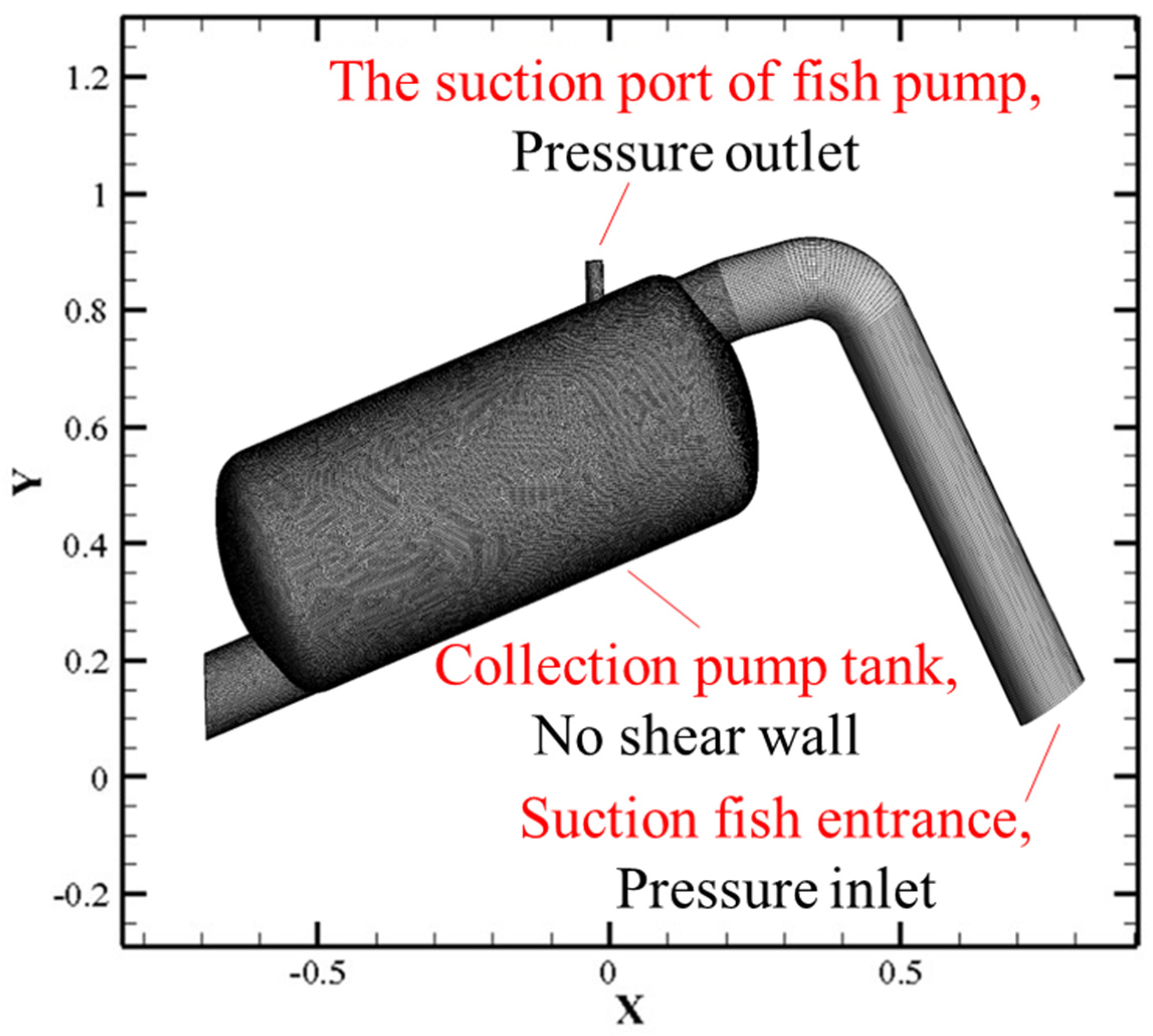
As shown in
Figure 2, the suction pump inlet, the pressure inlet boundary is selected, the initial pressure value is set according to the parameters of the vacuum pump, the fish outlet and the suction pump cavity are set as the fixed non-slip wall boundary, and the suction pump outlet is set as the pressure outlet boundary.
The CFD numerical of this study was realized based on a computational fluid dynamics commercial software FLUENT 2022R2. For the solution of unsteady flow field, the above partial differential equation is transformed into the solution of linear equations. Firstly, the finite volume method (FVM) of unstructured grids is used to discretize these partial differential equations, as shown in
Figure 2. For pressure–velocity coupling, the semi-implicit method of pressure–velocity coupling is used to discretize the convection term. Then, the pressure and momentum are spatially discretized by the second-order upwind difference scheme. The second-order implicit difference scheme is used for time discretization. Finally, the Gauss–Seidel iteration method is used to solve the algebraic equation by using an algebraic multigrid (AMG) solver. For the discretized continuous equation, momentum equation, and energy equation, the convergence criterion of the inner iteration is set to 10
−6.
To ensure the stability and convergence of the computation, a Courant–Friedrichs–Lewy number (
C0) should control to be less than 1, which can be defined as follows:
where
Umax is the maximum flow velocity,
Umax = 13 m·s
−1. The Δ
xMin is the minimum grid size, Δ
xMin = 7.5 × 10
−3 m. Δ
t is time step, Δ
t = 5 × 10
−4 s.
In order to verify the effectiveness of the above numerical method, the experiment device is shown in
Figure 3a, including a set of PIV systems (light source system, synchronization system, image capture system, image analysis system) and a physical model of vacuum fish pump made of transparent plexiglass. The specific arrangement of the experiment is shown in
Figure 3b, an optical camera is placed at the front end of the transparent fish pump, and a laser emitter is placed at the bottom to measure the cross-sectional velocity information of the measured flow field. There are four monitoring points (point A, point B, point C, point D) were set up on the middle section of the suction pump. The flow velocity values of the monitoring points under the pump pressure of 0.4 bar and constant pump pressure (equivalent inlet flow velocity v = 1 m/s) were measured, respectively, by an optical image analysis system. However, the tracer particles in the image will be misaligned when the fluid PIV experiment is carried out in a circular tube, and the measurement results deviate from the real flow velocity. In this regard, a linear image correction method is used to linearly scale the deformed image in the radial direction according to a certain proportion to correct the distorted image [
21]. The image correction uses a bilinear interpolation algorithm. When the distorted image is linearly corrected, it is scaled
n31 times in the radial direction, and
n31 can be calculated by the following formula:
where
n3 is the refractive index of air,
n3 = 1.0.
n1 is the refractive index of water,
n1 = 1.33. The slope of the initial section of the distortion curve has nothing to do with the material of the pipe but only with the refractive index of the medium in the pipe.
The main difference between the numerical simulation method of variable pressure and constant pressure vacuum fish pump is whether the pressure value of the initial pressure boundary is a constant value, and the other settings are completely consistent.
Table 2 is a comparative analysis of the water flow velocity results measured at monitoring points 1, 2, 3, and 4 under the numerical simulation and experimental methods of the constant pressure vacuum fish pump. It can be seen that the error between the experimental values and the numerical simulation results at the four monitoring points is small. At the same time, three kinds of mesh sizes (10
−3, 5 × 10
−4, 10
−4) corresponding to mesh 1, mesh 2, and mesh 3 are selected for mesh independence verification analysis. The results show that the selected mesh size achieves numerical convergence. In order to ensure the computational efficiency, the mesh size of 5 × 10
−4 m is selected in the subsequent numerical calculation.
Figure 4 is a comparative analysis of the numerical simulation of the variable pressure vacuum fish pump and the experiment results at the monitoring point A. It can be seen that the fish pump has the maximum speed at the monitoring point A when it starts to catch; that is, the fish pump has the maximum suction. With the increase in time, the speed at the monitoring point A gradually decreases, and the final speed decays to 0. At the same time, the experimental results are basically consistent with the numerical results, indicating the effectiveness of the numerical method of the variable pressure vacuum fish pump.
3.1.1. Numerical Simulation of Variable Suction of Fish Suction Pump
The internal liquid phase cloud diagram of the pump at 0–4 s when the vacuum fish pump is working, as shown in
Figure 5. It can be found that when the internal pressure of the fish pump is balanced with the external atmospheric pressure, the fish pump stops catching, and the internal water level of the pump reaches the highest value. With the increase in the pressure difference between the working pressure and the external pressure, the higher the internal water level of the pump, the higher the catching efficiency. Through quantitative analysis, it can be concluded that the total water body inside the fish pump is 1.947 m
3 when the working pressure is 0.1 bar, accounting for 92.7% of the pump; when the working pressure is 0.2 bar, the total water inside the fish pump is 1.476 m
3, accounting for 70.3% of the pump. When the working pressure is 0.3 bar, the total water inside the fish pump is 1.236 m
3, accounting for 58.8% of the pump. When the working pressure is 0.4 bar, the total water inside the fish pump is 0.846 m
3, accounting for 40.3% of the pump.
Figure 6a shows the velocity duration curve at the inlet of the vacuum pump. On the whole, with the increase in time, the fishing speed of the suction pump becomes lower and lower, and the speed is zero at about 3–3.5 s (the internal and external pressure difference is equal at this time). Because the water has inertial speed, it will increase again and then gradually decay to zero. At the same time, the attenuation of velocity shows obvious nonlinearity, and the larger the internal and external pressure difference is, the more obvious the nonlinearity is. With the increase in the internal and external pressure difference, the start-up speed and the average speed of the arrest are greater, and the time to reach the equilibrium time is longer. This also explains the reason why the higher the pressure difference between the external pressure and the working pressure in
Figure 5, the higher the internal water level of the pump.
The pressure duration curves at the inlet and outlet of the fish pump are shown in
Figure 7; it can be seen that the pressure at the inlet gradually increases with time and finally rises to the equilibrium value (external atmospheric pressure value). According to
Figure 6, the inlet velocity is 10–13 m/s at the initial time. If the live fish enters the suction pump at this high speed, there will be a great probability of damage or even death. In other words, it is difficult to control the suction by using this variable suction method. If the initial suction is too large, it will cause damage to the live fish, and if the suction is too small, the capture efficiency is too low. For the above problems, we think that we can reduce the initial suction of the fish pump and control the continuous pumping of the fish pump to maintain a constant pressure difference inside and outside the fish pump. This is an effective measure to reduce the damage rate of the fish body without affecting the fishing efficiency.
3.1.2. Numerical Simulation of Constant Suction of Fish Suction Pump
In order to verify the feasibility of the above ideas, the variation in the internal flow field of fish suction pump under constant pressure difference was simulated using the CFD method. The distribution of liquid volume fraction at different water injection speeds is shown in
Figure 7; it can be seen that the water level in the suction pump rises significantly more slowly than that in the suction pump with variable suction. When the pumping speed is 1 m/s, the total water inside the fish pump is 0.945 m
3, accounting for 45% of the pump at 15 s. When the pumping speed is 1.5 m/s, the total water inside the fish pump is 1.428 m
3, accounting for 68% of the pump at 15 s. When the pumping speed is 2.0 m/s, the total water inside the fish pump is 1.89 m
3, accounting for 90% of the pump at 15 s. As shown in
Figure 8, the main part of the impact of the fish body is the bottom of the suction pump, and the impact of the bottom of the suction pump is smaller with the increase in the water level. As the velocity increases, the impact point gradually moves away from the velocity inlet.
Obviously, using the control method of constant pressure difference can reduce the impact of the small fish body on the suction pump chamber, but the catching efficiency will be significantly reduced. From the perspective of live fish transportation, this suction method is more suitable.
3.2. Physical Experiment of Vacuum Fish Pump
The vacuum fish pump prototype was used to carry out the capture experiment of pond fish, as shown in
Figure 9. The experimental pond is mainly the grass carp, mixed carp, crucian carp, silver carp, and bighead carp. The vacuum fish pump is fixed horizontally on the bank of the pond. The center of gravity of the fish pump is about 1.5 m away from the shore and about 2.5 m from the water surface of the pond. The suction port of the fish suction pump is placed in the fish cage of the fish pool. The inner wall of the suction pipe is smooth and soft, and will not cause damage to the fish body. The vacuum fish suction pump in the aquaculture pond has initially realized the function of sucking fish with water. The fish suction time is 20 s, the fish release time is 10 s, and the fish suction and release operations are carried out in turn. Based on the numerical results, the experiment uses continuous pumping to keep the pressure difference between the inside and outside of the fish pump unchanged, which means that the fishing speed of the fish pump remains unchanged. In this experiment, the suction speed is 1, 2, and 3 m/s, respectively. Taking the suction speed of 1 m/s as an example, the average suction amount of the actual fish-water mixture was measured to be about 73 t after 1 h of operation and 120 cycles.
The vacuum fish pump experiment mainly performs performance experiments, including fish intake, cycle times, and fish body damage experiments. The fish body damage experiment mainly observes whether the fish body surface has bleeding, lack of scales, and scars. In order to further quantify the degree of fish damage, we propose a preliminary formula for calculating the fish damage rate applicable to vacuum suction pumps, as follows:
where
Fishdamage is fish damage due to vacuum suction pumps.
Sdamage is the sum of the areas on the fish with missing scales or scars.
SFish is surface area of the fish.
The single-tank vacuum suction pump experiment was carried out on grass carp, carp, crucian carp, silver carp, and bighead carp, and the detailed parameters of the experiment fish are shown in
Table 3. The results showed that the average single suction amount of crucian carp and carp was larger, and the average single suction amount of grass carp and bighead carp was smaller. The fish–water ratio was in the range of 1:1.5~1.68, and the dephosphorization of fish surface was observed. The damage rate of fish body was quantitatively analyzed from the dephosphorization of fish body surface. As shown in
Figure 10, the damage rates of grass carp, silver carp, and bighead carp were 2%, 0.3%, and 0.1%, respectively, under the condition of suction speed of 1 m/s. Carp and crucian carp were not damaged, and the average suction volume of the suction pump was about 23 t/h. Under the condition of suction speed of 1.5 m/s, the damage rates of grass carp, carp, silver carp, and bighead carp were 3%, 0.3%, 0.7%, and 0.3%, respectively. Crucian carp was not damaged, and the average suction volume of suction pump was about 28 t/h. Under the condition of suction speed of 2 m/s, the damage rates of grass carp, carp, crucian carp, silver carp, and bighead carp were 5%, 1%, 0.5%, 1%, and 0.5%, respectively, and the average suction volume of the suction pump was about 36 t/h. The actual total amount of fish suction was low in the experiment due to the performance of vacuum pump, the influence of sealing performance of fish suction pump, and the fish–water ratio.
The suction capacity of the fish pump corresponding to the three suction speeds is about 23 t/h, 28 t/h, and 36 t/h, respectively, which has a certain gap with the design value. This is mainly due to the performance of the vacuum pump, the sealing performance of the fish pump, and the small fish–water ratio. With the increase in suction speed, the average weight of single suction increases gradually, and this increase does not show a geometric multiple growth relationship according to the increase in suction speed. In addition, the damage rate of the fish body also increases with the increase in suction speed. It can be seen from
Table 4 that the damage rate of fish with relatively small size is relatively low. For example, crucian carp did not appear damaged until the suction speed reached 2 m/s, and the damage rate was only 0.5%. Common carp did not appear damaged until the suction speed reached 1 m/s, and the damage rate was only 0.3%. Grass carp is longer and easier to scale than common carp, crucian carp, silver carp, and bighead carp. The damage rate was 5% at a high suction speed (v = 2 m/s). This shows that the degree of damage to the fish body depends largely on the hardness of its own scales and the size of the fish body. The larger the size of the fish body, the more likely it is to be damaged during high-speed transport. The damage rate of fish body at the suction speed of 1 m/s meets the actual demand, so it is the best suction speed. The working efficiency of the fish suction pump mainly depends on the flow velocity of the suction pipe and the fish–water ratio of the fish collection system. The greater the flow velocity, the greater the suction volume per unit time of the suction pump, and the higher the working efficiency; the working efficiency of the vacuum fish pump is not only related to the flow velocity but also closely related to the fish–water ratio. Studies have shown that when the fish–water ratio is 1:1, the best fish absorption effect can be achieved. The fish–water ratio of the suction pump in this study is small, in the range of 1:1.5~1.68. When the suction pump begins to pump, the fish–water ratio is large, but as the suction progresses, the fish–water ratio in the fish collection system will gradually decrease, affecting the efficiency of the suction pump. In order to improve the working efficiency of the fish pump, it is necessary to develop an efficient fish collection device in the subsequent research, which can maintain the fish–water ratio at a certain level. In addition, it is also a meaningful measure to carry out research on the double-tank vacuum fish pump.
In order to obtain the efficiency of the vacuum suction pump, the electrical energy consumed and the total mass of live fish caught by the vacuum suction pump in one hour of continuous operation were measured. The efficiency of the vacuum fish suction pump can be calculated according to Equation (4). The calculation results of the efficiency of the vacuum fish pump under three suction speeds and fish–water ratios are shown in
Table 4. It can be clearly seen that under the condition of a certain fish–water ratio, its efficiency gradually decreases with the increase in the suction speed of the suction pump. As the fish suction pump fish–water ratio increases, the efficiency of the vacuum fish suction pump also gradually increases when the suction speed is 1 m/s. This is because as the fish–water ratio increases, the fish discharge time (t
2) will increase, while the fish suction time (t
1) will be shortened. As a result, the actual pumping operation time of the vacuum pump becomes shorter, i.e., the power consumption becomes less. Although the total mass of live fish pumped also decreases as the fish–water ratio increases, the reduction is not as great as the reduction in electrical energy consumption. Therefore, the efficiency of the vacuum suction pump increases as the fish–water ratio increases.


