A Method for Aliasing Metal Particle Recognition Based on Three-Coil Sensor Using Frequency Conversion

Abstract

The diesel engine on a ship is crucial as it serves as the primary power source, significantly influencing both the vessel’s efficiency and safety. Monitoring metal wear particles found in lubricating oil is essential for assessing the lubrication condition of mechanical equipment onboard and anticipating potential failures. Analyzing these metal wear particles allows us to gauge the wear status of bearing pairs within the machinery, thereby providing a technical foundation for routine maintenance activities. However, under real operating conditions, it can be challenging to prevent multiple metal particles from simultaneously passing through sensors. To address this issue, this research introduces an innovative three-coil induction sensor that employs a variable-frequency excitation technique to explore how induction and eddy currents interact. The findings indicate that when the excitation frequency changes, the peak value of the signal from 337 μm iron particles only increases by 3.35 times, while the peak value of the signal from 340 μm copper particles increases by 22.69 times. Consequently, this study recommends using changes in excitation frequency to differentiate between mixed metal particles made of various materials.

1. Introduction

The complexity of large equipment renders the identification of damaged parts exceedingly challenging. During the operation of mechanical components, wear particles will be generated between the friction pairs due to relative motion. The wear particles contain valuable information regarding the mechanical equipment [1,2,3]. Therefore, through an analysis of the material composition, size distribution, and quantity of these particles in the lubricating oil, it is possible to evaluate the wear condition of the mechanical equipment and accurately determine its location [4,5,6].

In recent years, researchers have conducted extensive studies on methods for detecting wear particles. Common methods include the capacitance method, inductance method, resistance method, optical method, acoustic method, and visual method [7,8,9,10,11]. The optical and acoustic methods can detect very small particles and have high detection sensitivity, providing information on the shape of the particles. However, the detection equipment for these methods is usually expensive and requires special maintenance and calibration. It may also be affected by the color, transparency, and optical properties of the sample, and because of its own limitations, it cannot identify the material of the wear particles. In wear state monitoring, the inductance method is often used. Common inductive sensors include single-coil, dual-coil, and triple-coil sensors [12,13]. The inductive sensors are capable of distinguishing between ferromagnetic metal wear particles and non-ferromagnetic metal wear particles. The inductive detection method focuses on enhancing detection accuracy and increasing throughput by incorporating high-conductivity materials, designing responsive detection circuits, and modifying the coil structure [14,15,16].

In recent years, most researchers have focused on improving the sensitivity of detecting worn particles. Rayne et al. [17] developed a novel eddy current particle sensor that uses an excitation coil and multiple induction coils to detect iron magnetic particles with a diameter of 120 microns and non-magnetic particles with a diameter of 210 microns. Zhang et al. [18] proposed a short solenoid-type inductive sensor that can detect iron particles with a diameter of 50 microns and copper particles with a diameter of 100 microns. However, in actual operating environments, iron particles and copper particles often overlap. Ma et al. [19] studied the superimposed signal characteristics of sensed particles when multiple particles passed through an inductive particle detection sensor. They studied the effects of the spacing, size, and magnetic properties of overlapping particles on the inductive signal. Wang et al. [20] proposed a method based on cross-correlation to establish a mathematical model for analyzing the overlapping behavior of particle signals and evaluating the severity of the overlapping problem. They studied and analyzed multi-particle overlapping signals but were still unable to achieve accurate identification. Li et al. [21] used a convolutional neural network (CNN)-based degradation mixture estimation technique (DUET) to separate features from overlapping signals and identify the magnetic properties of mixed particles. Li’s research used idealized case signals, and the effectiveness of this method would decrease in more complex situations. Isaac Opeyemi Olalere [22] and Kenan Shen [23] et al. identified metal chips using neural networks from a software perspective, but the recognition results were highly dependent on the dataset, and poor recognition results were obtained in changing operating conditions, lacking a certain degree of universality. Furthermore, they did not study overlapping chips.

Currently, most methods used for identifying overlapping particles require processing complex signals, while overlapping signals themselves are difficult to handle, resulting in low accuracy and efficiency. They usually require a large amount of computing resources. The identification method mentioned in this paper starts from the physical properties of metal abrasive particles and uses the sensitivity of ferromagnetic and non-ferromagnetic abrasive particles to magnetic field frequencies to obtain amplitude differences and thus obtain the signal state of overlapping particles, thereby achieving the identification of mixed particles. This method has a high accuracy rate and low computing requirements, which is of great significance for real-time monitoring and identification of metal abrasive particles.

2. Modeling and Simulation

This study uses an inductive three-coil oil metal particle detection sensor, as shown in Figure 1, with three solenoid coils in the lubricating oil flow pipe, where the two side coils are the excitation coils and the middle one is the induction coil. The side coils are connected in the opposite direction and a sinusoidal voltage excitation source is added. The magnetic fields generated by the excitation coils, which have identical parameters but opposite directions, mutually cancel each other out, resulting in a null magnetic flux density at the center of the induction coil. The passage of metal particles through the induction coil causes a modification in the internal magnetic field, resulting in the generation of an induced voltage that exhibits a sinusoidal waveform.

This study simulated the movement of metal particles through an inductive three-coil sensor using COMSOL Multiphysics 6.1 software. The magnetization and eddy current effects were investigated separately using iron and copper particles to examine their response to different excitation frequencies. The model parameters established in the simulation were consistent with the experimental parameters. Three identical solenoid coil windings were used, with a height of 1 mm, an outer diameter of 7.2 mm, an inner diameter of 3.5 mm, and 300 turns of wire. The model was arranged in a triangular configuration, as depicted in Figure 2, with the adjacent coils spaced at a distance of 0.1 mm. In most studies on detecting metal particles, to simplify calculations, standardize procedures, and facilitate experimental operations, most researchers equated metal particles with spherical particles for experiments. In this simulation, the modeling of metal particles also used standard spherical particles.

The properties of metal particles are determined by measuring changes in the signal amplitude from identical metal particles while varying the intensity of the alternating magnetic field. The addition of an alternating excitation signal to the coil results in the generation of a dynamic magnetic field. Both magnetization and eddy current effects influence the behavior of metal particles in an alternating magnetic field. The impact of the alternating magnetic field on spherical metal particles depends on factors such as the excitation frequency, the complex magnetic susceptibility coefficient of the particles, the coil structure, and the number of coil turns.

From Figure 2, the effect of metal abrasive particles on the coil when they pass through the induction coil can be observed. Iron abrasive particles mainly exhibit a magnetization effect, with the magnetic flux density of the abrasive particle being higher than that of the coil; copper abrasive particles mainly exhibit an eddy current effect, with the magnetic flux density of the abrasive particle being lower than that of the coil. When both iron and copper abrasive particles pass through the coil at the same time, the magnetic flux density of the iron abrasive particle is greater than that of the coil, and the coil is greater than that of the copper abrasive particle. The scale values reflect the degree of magnetization or eddy current.

According to previous studies [24,25,26], Formula (1) can be utilized to compute the variations in the inductance and resistance values of a spherical monocrystalline metal particle when it enters a pulsating magnetic field.

$$\mathsf{\Delta }L=I_m\left({\displaystyle \frac{\Delta Z_{max}}{\omega }}\right)=0.5A{\mu }_0{\left[{\sum }_{\left(m=1\right)}^M{\displaystyle \frac{P_m\left(Z_0\right)}{W^2}}\right]}^2{R}_e\left(K_p\right)$$

(1)

where $\mathsf{\Delta }{Z}_{max}$ represents the equivalent impedance peak caused by the metal particles, $\omega$ is the angular frequency of the alternating current, $A$ is the amplification factor caused by the change in electrical inductance due to the position of metal particles, ${\mu }_0$ is the vacuum permeability, $M$ is the number of turns in the coil, $Z_0$ is the distance from the center of the metal particle to the surface of the planar coil, $W$ is the inner diameter of the coil, and $K_p$ is the complex magnetic susceptibility of metal abrasives, including factors such as the excitation source frequency, particle size, and the electromagnetic properties of the particles.

The expression for the composite magnetization coefficient $K_{p1}$ of ferromagnetic metal particles in a pulsating magnetic field is:

$$K_{p1}={\displaystyle \frac{a^3}{2}}{\displaystyle \frac{\left(-a^2{k}^2+2{\mu }_r+1\right)\mathit{sin}\left(ak\right)-ak\left(2{\mu }_r+1\right)\mathit{cos}\left(ak\right)}{\left(a^2{k}^2+{\mu }_r-1\right)\mathit{sin}\left(ak\right)-ak\left({\mu }_r-1\right)\mathit{cos}\left(ak\right)}}$$

(2)

For non-ferromagnetic metallic abrasives, relative permeability ${\mu }_r=1$, and the expression for the composite magnetization coefficient $K_{p2}$ is given by:

$$K_{p2}=-{\displaystyle \frac{1}{2}}\left[a^3+{\displaystyle \frac{3a^2}{k}}\mathit{cot}\left(ak\right)-{\displaystyle \frac{3a}{k^2}}\right]$$

(3)

The formula for $k$ is:

$$k=\sqrt{-j\omega {\mu }_r{\mu }_0\sigma }$$

(4)

In this equation, $a$ represents the radius of the metal abrasive particle, $\omega$ is the angular frequency of the alternating current (AC) voltage, ${\mu }_r$ is the relative permeability of the metal abrasive, ${\mu }_0$ is the vacuum permeability, and $\sigma$ is the electrical conductivity of the metallic abrasive. The above formula reveals a complex relationship between the impedance, inductance, and voltage variations of ferromagnetic and non-ferromagnetic metal particles passing through the coil, which is intricately linked to both particle size and excitation frequency.

We can see that the vacuum permeability ${\mu }_0=4000$, the relative permeability of iron particles ${\mu }_{r1}=6.30\times 10^{-3}\mathrm{H}/\mathrm{m}$, the relative electrical conductivity ${\sigma }_1=1.04\times 10^7\mathrm{S}/\mathrm{m}$, the relative permeability of copper particles ${\mu }_{r2}=1.26\times 10^{-6}\mathrm{H}/\mathrm{m}$, and the relative electrical conductivity ${\sigma }_2=5.98\times 10^7\mathrm{S}/\mathrm{m}$.

The results of Formulas (2)–(4) indicate that there is a direct correlation between the size of the ferromagnetic and non-ferromagnetic metal abrasive particles and the magnitude of the hysteresis coefficient change. The hysteresis coefficient of the ferromagnetic metal abrasive particles remains unchanged with variations in excitation frequency. In contrast, the hysteresis coefficient of the non-ferromagnetic metal abrasive particles exhibits a relatively significant change. This is because magnetization effects primarily influence ferromagnetic metals in the presence of a magnetic field. In contrast, non-ferromagnetic metals are predominantly affected by eddy current effects, which are closely associated with the excitation frequency. The distinct responses of ferromagnetic and non-ferromagnetic metal particles to the excitation frequency enable us to differentiate their overlapping characteristics.

When both iron and copper metal particles enter the sensor simultaneously, the metal particles interact with each other. The interaction between the two metal particles is disregarded to simplify the model. Consequently, the expression for the composite magnetization coefficient of the overlapping metal particles is as follows:

$$\mathsf{\Delta }{K}_p=K_{p1}\times K_{p2}$$

(5)

This present section employs COMSOL software to conduct a simulation analysis, investigating the voltage variations induced by 200 μm iron particles and 400 μm copper particles as they traverse the sensor coil at different excitation frequencies. Furthermore, it examines the correlation between the composite magnetic susceptibility of overlapping metal particles and excitation frequency and particle size. The proposed method’s feasibility has been validated.

The magnetic field density distribution was simulated using COMSOL software, as depicted in Figure 3a. Under the influence of the alternating magnetic field, the iron particles primarily experience magnetization effects, thereby amplifying the original magnetic field. The copper particles primarily experience the eddy current effect, resulting in a reduction of the initial magnetic field strength. The voltage changes caused by the two metal particles passing through the sensor at excitation frequencies of 10 kHz and 90 kHz are illustrated in Figure 3b. It can be observed that the voltage output of the iron particles changes very little under the influence of the two excitation frequencies. This is because the influence of the excitation frequency on the magnetization effect is lower and the influence on the eddy current effect is higher. Therefore, the output signal of the copper particles is not obvious under the 10 kHz excitation frequency, and the output signal is significantly increased and stable under the 90 kHz excitation frequency.

3. Experimental System Design

To accurately simulate the motion state of metal particles in the oil, the method of attaching the metal particles to nylon thread with glue was used so that they could pass through the made sensor for observation. The entire experimental platform system is shown in Figure 4, which consists of the metal particle motion control system and the metal particle signal acquisition system. The motion control system comprises a three-axis fine adjustment platform (LD60-LM-2) and a precision sliding platform (FSL40). The LD60-LM-2 precisely regulates the positioning of the sensor throughout the entire experimental platform, ensuring the accurate passage of metal particles through the sensor coil; meanwhile, the FSL40 controls and coordinates the reciprocating motion of these metal particles. The movement speed of the metal particles through the coil will also impact the output signal; therefore, to obtain consistent induced signals and identify general patterns, it is necessary to ensure that the metal particles pass through the sensor at a uniform velocity during the experiment. The signal acquisition system consists of an impedance analysis board and a computer. The impedance analysis board will add fixed frequency voltage excitation to the sensor coil and continuously acquire the induced signal of the sensor. The computer uses LabVIEW 2017 software to visualize and save the signals collected by the impedance analysis board.

4. Experiment on the Frequency of Metal Particles

In this experiment, conventional ferromagnetic particles and non-ferromagnetic particles, namely iron particles and copper particles, were selected. Qualified metal particles were selected through microscopic screening. To facilitate observation, regular, spherical metal particles with standard sizes were typically chosen. The inductance signal of the metal particles was detected using the experimental system shown in Figure 4. The sizes of the metal particles involved in the experiment are shown in

Table 1. List of metal particles required for the experiment.

Particle Samples	Particle Size
Iron particles	88 μm	133 μm	155 μm	170 μm	337 μm
Copper particles	280 μm	340 μm	500 μm	600 μm	700 μm
Aliasing particles 1	80 μm Fe +280 μm Cu	88 μm Fe +340 μm Cu	80 μm Fe +500 μm Cu	88 μm Fe +600 μm Cu	83 μm Fe +700 μm Cu
Aliasing particles 2	75 μm Fe +340 μm Cu	109 μm Fe +340 μm Cu	178 μm Fe +340 μm Cu	255 μm Fe +340 μm Cu	320 μm Fe +340 μm Cu
Aliasing particles 3	88 μm Fe +600 μm Cu	116 μm Fe +600 μm Cu	170 μm Fe +600 μm Cu	257 μm Fe +600 μm Cu	334 μm Fe +600 μm Cu

.

Microscopes were used to select metal particles that met the required specifications for sample preparation. Due to the difficulty in finding metal particles of exactly the same size, some samples were prepared using particles of similar size instead. Some metal wear particles were observed under a microscope, as shown in Figure 5.

4.1. Study of Iron Particle Frequency Characteristics

The impact of excitation frequency on the properties of ferromagnetic particles is investigated, and Figure 6 illustrates the correlation between excitation frequency and the characteristics of an individual iron particle.

From Figure 6, it can be seen that the amplitude of the induced sensor voltage signal increases with the size of a single iron particle at 10 kHz and 90 kHz excitation frequencies. This is because the excitation frequency has a multi-faceted effect on metal particles, the most important of which are the magnetization effect and the eddy current effect, with the magnetization effect having a much greater influence on ferromagnetic metal particles than the eddy current effect. As shown in Figure 7, when a 337 μm iron particle is examined separately, its voltage amplitude is 5009 μV at 10 kHz excitation frequency and 16,766 μV at 90 kHz excitation frequency—approximately 3.35 times. This indicates that the excitation frequency impacts the sensor voltage output for ferromagnetic particles.

Figure 8 shows an experimental frequency measurement of an 88 μm iron particle to further illustrate this phenomenon.

The experiment selected a single iron sphere with a diameter of 88 μm and added the range of 10–100 kHz with 10 kHz interval excitation frequencies to observe the voltage increase. The iron particle’s voltage increase is insignificant at the range of 10–60 kHz. However, a zero-drift phenomenon occurs at an excitation frequency of 80 kHz. The voltage increase is evident at excitation frequencies of 90 kHz and 100 kHz. The smallest voltage increase occurs at an excitation frequency of 40 kHz. Experimental results demonstrate that the relationship between excitation frequency and voltage increase is not linear. Different coil structures and parameters correspond to their respective optimal excitation frequencies for achieving maximum voltage increase.

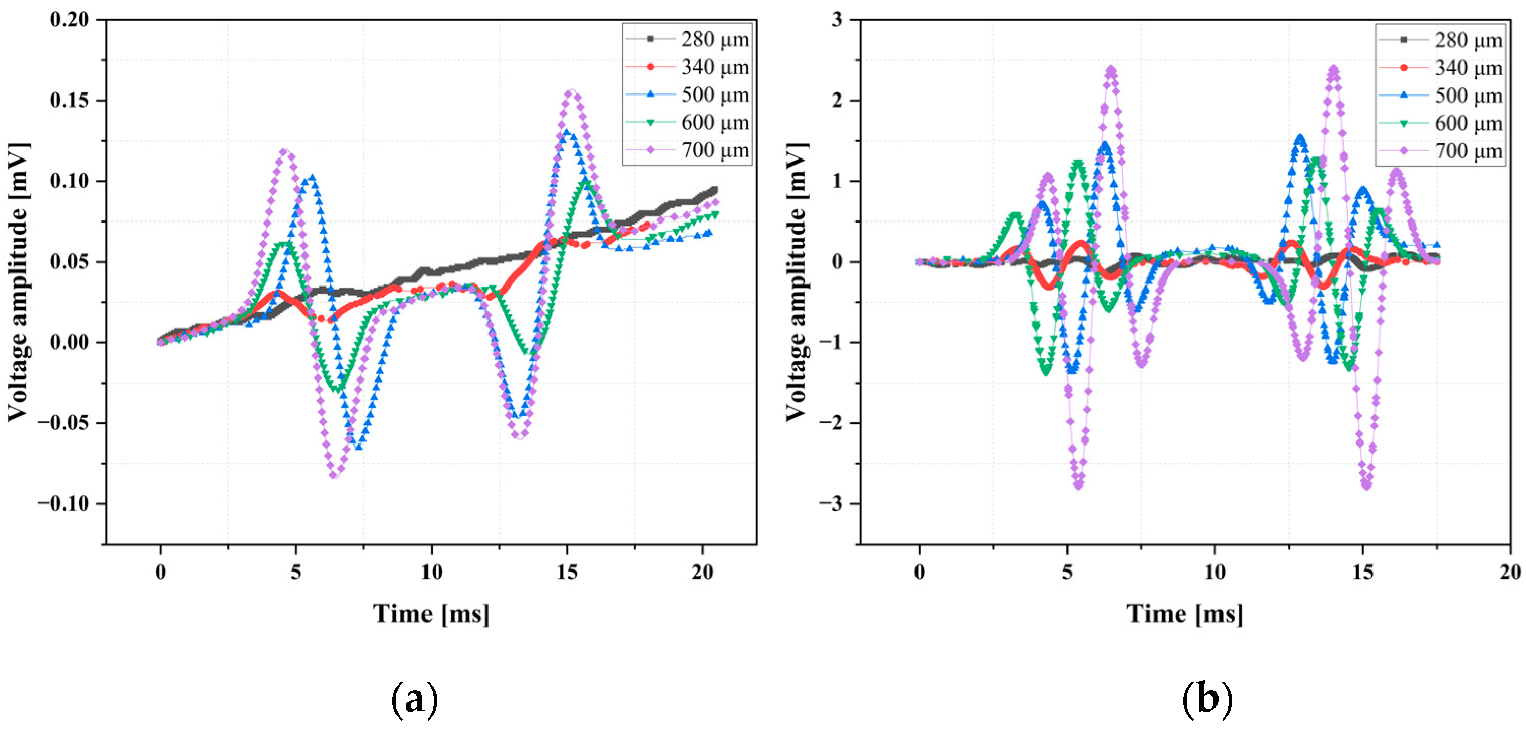
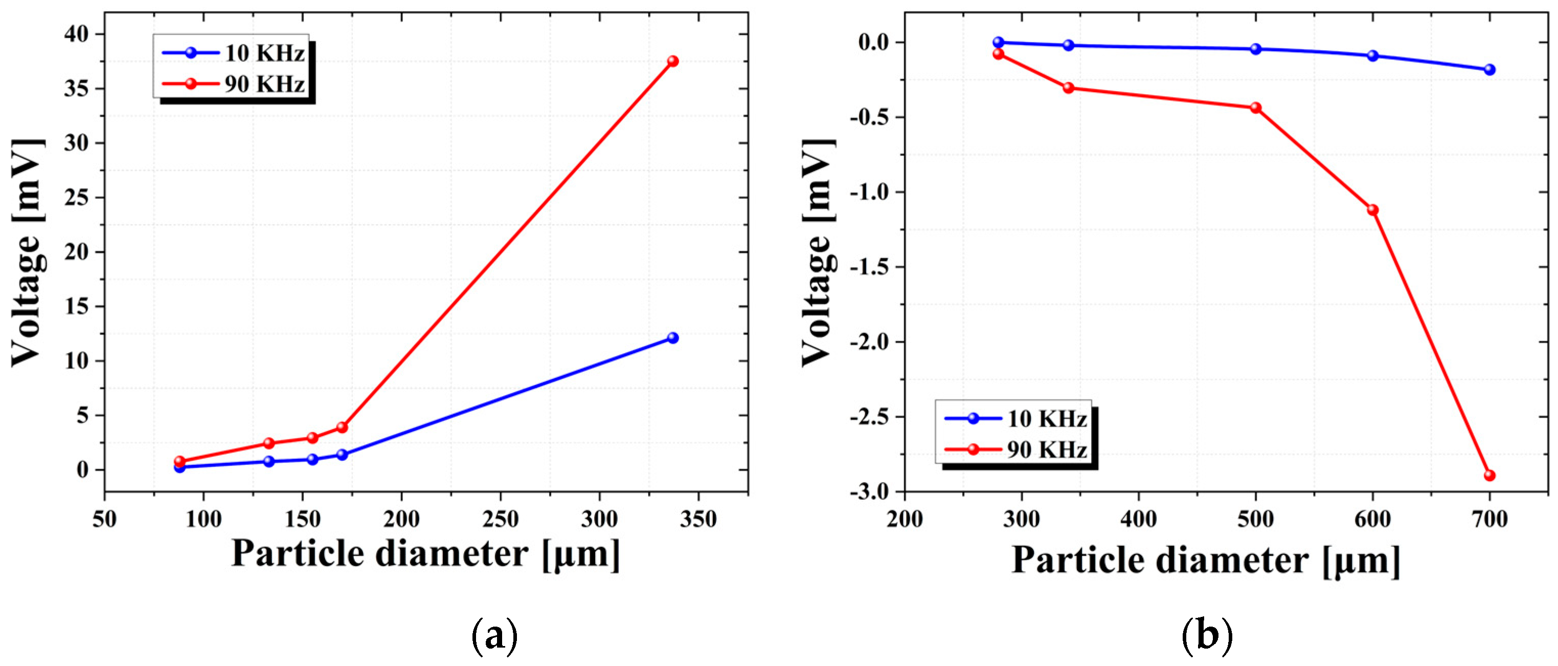
4.2. Study of Copper Particle Frequency Characteristics

To investigate the effect of excitation frequency on the properties of non-ferromagnetic particles, experiments were conducted using the most common non-ferromagnetic metal particles found in ship-lubricating oil, namely copper particles. The relationship between a single copper particle and the excitation frequency is shown in Figure 9.

The experiment selected a single copper particle with a diameter of 340 μm and added the range of 10–100 kHz with 10 kHz interval excitation frequencies to observe the voltage increase. The experimental results are shown in Figure 10. At a 10 kHz excitation frequency, there is a serious zero-point drift in the voltage signal, as low excitation frequencies are difficult to generate eddy current effects and the detection effect on copper particles is poorer. Therefore, in most sensors, the detection of copper particles is performed using higher excitation frequencies. At an excitation frequency of 50 kHz, a noticeable increase in the base noise was observed compared to other signals. At 60 kHz, 90 kHz, and 100 kHz excitation frequencies, the signal was clear and stable, and the amplitude reached its maximum at 100 kHz. The experimental results show that a single copper metal particle does not produce a stable and distinct signal at low excitation frequencies. As the excitation frequency is increased, a stable signal is produced and the signal amplitude can be greatly increased. The primary reason for this phenomenon is that the copper particles in the magnetic field primarily experience the eddy current effect, which is influenced by the excitation frequency. The stronger the eddy current effect, the greater the attenuation of the voltage signal amplitude. By adjusting the excitation frequency of the sensor, we can effectively detect and differentiate mixed metal particles consisting of ferromagnetic and non-ferromagnetic metals.

The increase in the size of the metal particles is observed to result in a corresponding amplification of the output voltage signal, as evidenced by Figure 7 and Figure 11, at both excitation frequencies of 10 kHz and 90 kHz. The correlation between particle size and the variation in output voltage signal at the two excitation frequencies is illustrated in Figure 12.

The relationship between the particle size of iron particles and the output voltage is illustrated in Figure 12a, while Figure 12b depicts the same relationship for copper particles. Both metal particles’ voltage signal output changes exhibit a greater magnitude at an excitation frequency of 90 kHz compared to that at 10 kHz. Moreover, as the size of the metal particles increases, the magnetization effect of iron particles demonstrates a slight enhancement at a frequency of 10 kHz and a significant enhancement at a frequency of 90 kHz. The eddy current effect of copper particles is not readily discernible at a 10 kHz excitation frequency but it becomes significant when the excitation frequency is increased to 90 kHz.

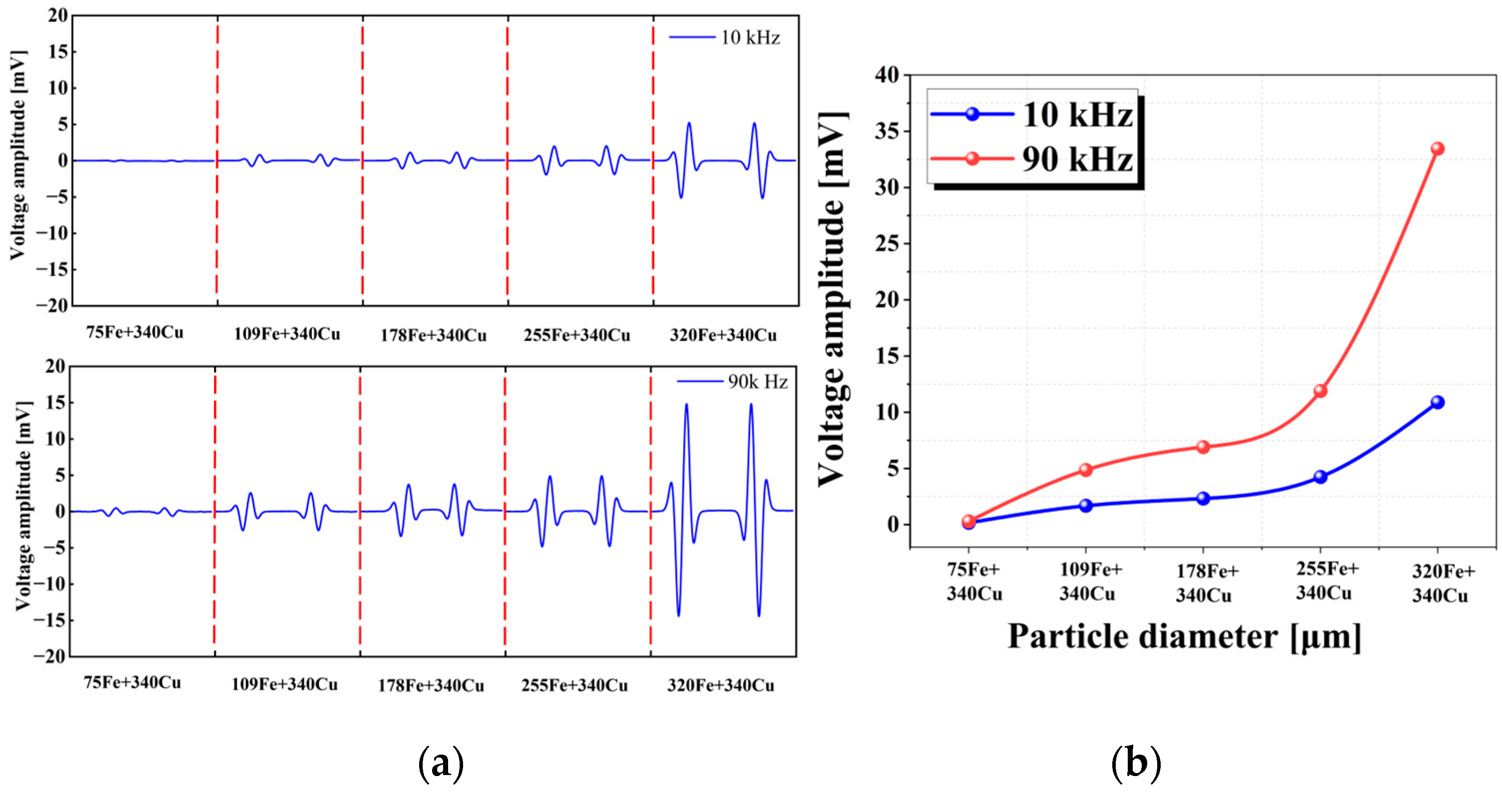
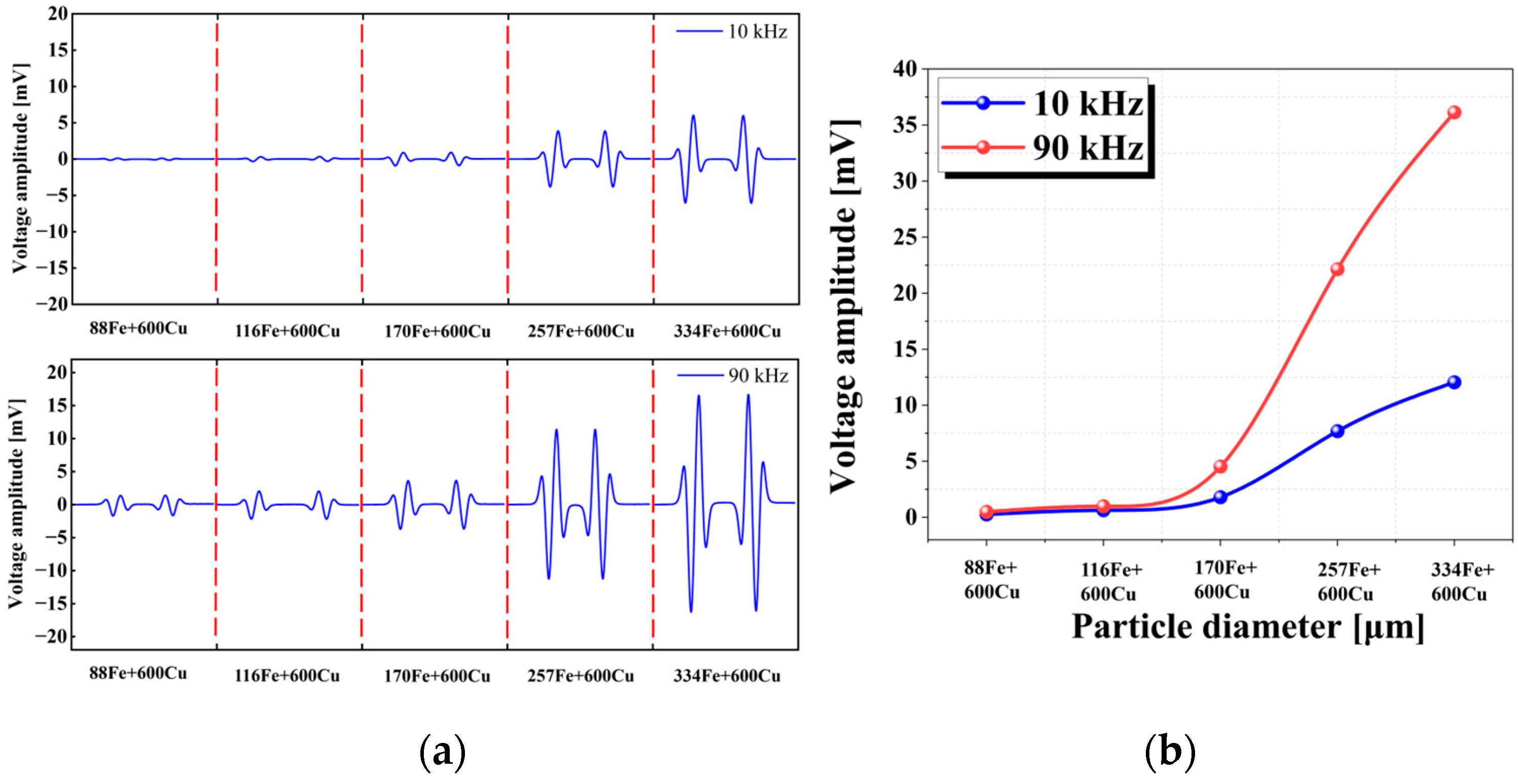
4.3. Frequency Characteristics of Metal Particles with Mixed Attributes

Upon entering the sensor, the arrangement of multiple particles impacts the output signal; however, once all particles have fully entered the sensor, their cumulative effect is reflected in the output signal.

The frequency experiments conducted on iron particles, copper particles, and mixed metal abrasives reveal that when comparing Figure 12, Figure 13, Figure 14 and Figure 15, it can be observed that iron particles exhibit commendable detection accuracy even at a 10 kHz excitation frequency. In contrast, copper particles demonstrate minimal signal amplitude under the same conditions. Therefore, only the iron particles will influence the output signal when iron and copper particles overlap and pass through the sensor at an excitation frequency of 10 kHz. At an excitation frequency of 90 kHz, both iron and copper particles have a discernible impact on the output signal, resulting in a superposition of signals from both types of particles. Consequently, by comparing the amplitude of the sensor’s output signal under different excitations, it becomes feasible to determine whether a mixture of particles has traversed.

5. Discussion

Stacking ferromagnetic and non-ferromagnetic particles in conjunction with their passage through a sensor results in the simultaneous amplification and attenuation of the magnetic field due to the combined effects of eddy currents and magnetization. Consequently, this leads to a diminished signal, causing the sensor to perceive it as a smaller particle. Metal abrasive detection poses a critical challenge, necessitating an urgent resolution for inductive sensors. Given the complexity of detecting multiple particle mixtures using inductive detection sensors, this paper proposes a variable-frequency detection method. By leveraging the distinct effects of magnetization and eddy currents in a variable-frequency magnetic field, it enables the detection of a mixture comprising ferromagnetic and non-ferromagnetic metal abrasive particles. The experimental results demonstrate that when two ferromagnetic particles traverse the sensor, distinct signals are observed at excitation frequencies of 10 kHz and 90 kHz, with a slight increase in the peak values of both signals. The signal peak value growth for the 337 μm iron particle is 3.35 times.

Conversely, when two copper particles pass through the sensor, no clear signal is detected at an excitation frequency of 10 kHz; however, a conspicuous signal emerges at an excitation frequency of 90 kHz, accompanied by a significant amplification in the two signal peak values. The signal peak value growth of the 340 μm copper particle is amplified by a factor of 22.69. When iron and copper particles pass through the sensor, a distinct signal is observed at an excitation frequency of 10 kHz; however, the signal peak value is relatively small. Conversely, at an excitation frequency of 90 kHz, there is a clear signal with significantly increased peak values. Three mixed particle samples correspond to three variable-frequency signals, which can be utilized for mixed particle identification. The commonly employed approach in the market for identifying mixed abrasive particles involves utilizing various algorithms to detect mixed signals. However, the variable-frequency method fundamentally transforms the challenge of identifying complex mixed signals and paves a new path for particle identification. Moreover, it offers a novel data acquisition method that can be utilized with diverse machine learning techniques to decompose mixed signals in future applications. Nevertheless, when multiple abrasives are present within a magnetic field, the situation becomes more intricate due to mutual forces exerted among them, resulting in non-linear additive behavior within the magnetic field. There are still many limitations in this study. Due to the maximum excitation frequency of the signal acquisition card being only 100 kHz, experiments with excitation frequencies of 10 kHz and 90 kHz were conducted, which does not represent the optimal detection frequency for this method. In addition, in real-world situations, metal particles have various shapes, and their modeling and simulation analysis is more complex. Therefore, in future research, studies should be conducted on other complex-shaped metal particles.

6. Conclusions

The primary challenge in detecting mixed metal particles using the inductive method lies in amalgamating metal particles with different attributes. Suppose two particles of the same attribute enter the sensor simultaneously. In that case, their signals will be added together to produce a larger signal, which we can consider to be a larger particle. Because they are difficult to separate in subsequent oil fluid, they also greatly impact the sensor’s detection. The primary focus of this paper is to address the challenge associated with detecting mixed metal particles that enter the sensor with different attributes. It conducts experiments on single iron and copper particles’ frequency characteristics, aiming to explore the correlation between particle size and output voltage at excitation frequencies of 10 kHz and 90 kHz. The frequency characteristic experiments of mixed iron and copper particles are also conducted to investigate the correlation between mixed particles and frequency variations at excitation frequencies of 10 kHz and 90 kHz. The output curves for different attribute metal particles under various excitation frequencies are obtained through simulation calculations, followed by experimental verification. The experimental results demonstrate that mixed metal particles with different attributes can be distinguished by altering the frequency, thereby providing a simple and stable method for identifying such particles. This approach offers a novel idea and technique for identifying mixed metal particles, which is an essential technical tool for intelligent monitoring and fault diagnosis of precise mechanical equipment. It significantly enhances equipment reliability, prolongs service life, and reduces maintenance costs.

References

1. Lu, P.; Powrie, H.E.; Wood, R.J.; Harvey, T.J.; Harris, N.R. Early wear detection and its significance for condition monitoring. Tribol. Int. 2021, 159, 106946. [Google Scholar] [CrossRef]
2. Li, Y.; Wu, J.; Guo, Q. Design on Electromagnetic Detection Sensor on Wear Debris in Lubricating Oil. In Proceedings of the 2019 IEEE International Instrumentation and Measurement Technology Conference (I2MTC), Auckland, New Zealand, 20–23 May 2019; IEEE: Piscataway, NJ, USA; pp. 1–5. [Google Scholar] [CrossRef]
3. Han, W.; Mu, X.; Liu, Y.; Wang, X.; Li, W.; Bai, C.; Zhang, H. A Critical Review of On-Line Oil Wear Debris Particle Detection Sensors. J. Mar. Sci. Eng. 2023, 11, 2363. [Google Scholar] [CrossRef]
4. Kattelus, J.; Miettinen, J.; Lehtovaara, A. Detection of gear pitting failure progression with on-line particle monitoring. Tribol. Int. 2018, 118, 458–464. [Google Scholar] [CrossRef]
5. Jia, R.; Wang, L.; Zheng, C.; Chen, T. Online Wear Particle Detection Sensors for Wear Monitoring of Mechanical Equipment—A Review. IEEE Sens. J. 2022, 22, 2930–2947. [Google Scholar] [CrossRef]
6. Chuma, E.L.; Iano, Y.; Roger, L.L.B.; de Oliveira, G.G.; Vaz, G.C. Novelty Sensor for Detection of Wear Particles in Oil Using Integrated Microwave Metamaterial Resonators With Neodymium Magnets. IEEE Sens. J. 2022, 22, 10508–10514. [Google Scholar] [CrossRef]
7. Zhang, L.; Yang, Q. Investigation of the Design and Fault Prediction Method for an Abrasive Particle Sensor Used in Wind Turbine Gearbox. Energies 2020, 13, 365. [Google Scholar] [CrossRef]
8. Roylance, B.J.; Williams, J.A.; Dwyer-Joyce, R. Wear debris and associated wear phenomena—Fundamental research and practice. Proc. Inst. Mech. Eng. Part J J. Eng. Tribol. 2000, 214, 79–105. [Google Scholar] [CrossRef]
9. Ren, Y.J.; Zhao, G.F.; Qian, M.; Feng, Z.H. A highly sensitive triple-coil inductive debris sensor based on an effective unbalance compensation circuit. Meas. Sci. Technol. 2019, 30, 015108. [Google Scholar] [CrossRef]
10. Sun, Y.; Jia, L.; Zeng, Z. Hyper-Heuristic Capacitance Array Method for Multi-Metal Wear Debris Detection. Sensors 2019, 19, 515. [Google Scholar] [CrossRef]
11. Zhao, Y.; Ge, P.; Bi, W.; Zheng, J.; Lan, J. Machine vision online detection for abrasive protrusion height on the surface of electroplated diamond wire saw. Int. J. Adv. Manuf. Technol. 2022, 121, 7923–7932. [Google Scholar] [CrossRef]
12. Qian, M.; Ren, Y.J.; Feng, Z.H. Interference reducing by low-voltage excitation for a debris sensor with triple-coil structure. Meas. Sci. Technol. 2020, 31, 025103. [Google Scholar] [CrossRef]
13. Jia, R.; Ma, B.; Zheng, C.; Wang, L.; Du, Q.; Wang, K. Improvement of Sensitivity and Detectability of the Three-Coil Wear Debris Detection Sensor Using LC Resonance Method and Modified Lock-in Amplifier. Preprints 2017. [Google Scholar] [CrossRef]
14. Huang, H.; He, S.; Xie, X.; Feng, W.; Zhen, H. Research on the Influence of Coil LC Parallel Resonance on Detection Effect of Inductive Wear Debris Sensor. Sensors 2022, 22, 7493. [Google Scholar] [CrossRef] [PubMed]
15. Feng, S.; Yang, L.; Qiu, G.; Luo, J.; Li, R.; Mao, J. An Inductive Debris Sensor Based on a High-Gradient Magnetic Field. IEEE Sens. J. 2019, 19, 2879–2886. [Google Scholar] [CrossRef]
16. Kim, M.K.; Chung, D.D.L. Inductance-based sensing of surface roughness, with application to wear sensing. J. Mater. Sci. 2024, 59, 15816–15829. [Google Scholar] [CrossRef]
17. Ren, Y.J.; Li, W.; Zhao, G.F.; Feng, Z.H. Inductive debris sensor using one energizing coil with multiple sensing coils for sensitivity improvement and high throughput. Tribol. Int. 2018, 128, 96–103. [Google Scholar] [CrossRef]
18. Zhang, Y.; Cao, Y.; Si, E.; Zheng, L. Study on a High Sensitive Online Sensor for Wear Particles in Lubricant. J. Phys. Conf. Ser. 2019, 1237, 042082. [Google Scholar] [CrossRef]
19. Ma, L.; Zhang, H.; Xie, Y.; Shi, H.; Zheng, W. Investigation on the superimposed characteristics of aliasing signals by multiple wear particles. Tribol. Int. 2023, 178, 107909. [Google Scholar] [CrossRef]
20. Wang, X.; Sun, H.; Wang, S.; Huang, W. Cross-Correlation Algorithm-Based Optimization of Aliasing Signals for Inductive Debris Sensors. Sensors 2020, 20, 5949. [Google Scholar] [CrossRef]
21. Li, T.; Wang, S.; Zio, E.; Shi, J.; Yang, Z. Aliasing Signal Separation for Superimposition of Inductive Debris Detection Using CNN-Based DUET. In Proceedings of the 2019 14th IEEE Conference on Industrial Electronics and Applications (ICIEA), Xi’an, China, 19–21 June 2019; IEEE: Piscataway, NJ, USA; pp. 211–215. [Google Scholar] [CrossRef]
22. Olalere, I.O.; Olanrewaju, O.A. Tool and Workpiece Condition Classification Using Empirical Mode Decomposition (EMD) with Hilbert–Huang Transform (HHT) of Vibration Signals and Machine Learning Models. Appl. Sci. 2023, 13, 2248. [Google Scholar] [CrossRef]
23. Shen, K.; Zhao, D. An EMD-LSTM Deep Learning Method for Aircraft Hydraulic System Fault Diagnosis under Different Environmental Noises. Aerospace 2023, 10, 55. [Google Scholar] [CrossRef]
24. Li, Y.; Wu, J.; Guo, Q. Electromagnetic Sensor for Detecting Wear Debris in Lubricating Oil. IEEE Trans. Instrum. Meas. 2020, 69, 2533–2541. [Google Scholar] [CrossRef]
25. Xie, Y.; Shi, H.; Zheng, Y.; Zhang, Y.; Zhang, H.; Sun, Y.; Zhang, X.; Zhang, S. An Asymmetric Micro-Three-Coil Sensor Enabling Non-Ferrous Metals Distinguishment. IEEE Trans. Instrum. Meas. 2023, 72, 3508909. [Google Scholar] [CrossRef]
26. Wan, Z.; Wang, Y.; Du, C. A High Sensitivity and Throughput Inductive Debris Sensor Using a Built-In Planar Energizing Coil. IEEE Trans. Instrum. Meas. 2024, 73, 9501709. [Google Scholar] [CrossRef]
Figure 1. Modeling and rendering of sensors.
Jmse 12 02273 g001
Figure 2. Metal abrasive particles through the sensor simulation model.
Jmse 12 02273 g002
Figure 3. (a) The magnetic flux density of different metal abrasives in a magnetic field. (b) Voltage output changes of iron and copper particles under different excitation frequencies.
Jmse 12 02273 g003
Figure 4. Experimental platform system.
Jmse 12 02273 g004
Figure 5. Partial metal particle samples.
Jmse 12 02273 g005
Figure 6. The correlation between excitation frequency and the dimensions of individual iron particles. (a) Relationship between 10 kHz excitation and the size of individual iron particles. (b) Relationship between 90 kHz excitation and the size of individual iron particles.
Jmse 12 02273 g006
Figure 7. Voltage signals of 337 μm iron particle under different excitation frequencies.
Jmse 12 02273 g007
Figure 8. Characteristics of frequency changes in a single iron particle with a diameter of 88 μm.
Jmse 12 02273 g008
Figure 9. The relationship between the excitation frequency and the size of individual copper particles. (a) Relationship between 10 kHz excitation and the size of individual copper particles. (b) Relationship between 90 kHz excitation and the size of individual copper particles.
Jmse 12 02273 g009
Figure 10. Characteristics of frequency changes in a single copper particle with a diameter of 340 μm.
Jmse 12 02273 g010
Figure 11. Voltage signals of 340 μm copper particle under different excitation frequencies.
Jmse 12 02273 g011
Figure 12. The relationship between metal particle size and output voltage. (a) The relationship between iron particle size and output voltage. (b) The relationship between copper particle size and output voltage.
Jmse 12 02273 g012
Figure 13. (a) Output curves of the aliased particle sample 1 under two excitation frequencies. (b) Output variation curves of the aliased particle sample 1 under two excitation frequencies.
Jmse 12 02273 g013
Figure 14. (a) Output curves of the aliased particle sample 2 under two excitation frequencies. (b) Output variation curves of the aliased particle sample 2 under two excitation frequencies.
Jmse 12 02273 g014
Figure 15. (a) Output curves of the aliased particle sample 3 under two excitation frequencies. (b) Output variation curves of the aliased particle sample 3 under two excitation frequencies.
Jmse 12 02273 g015