The Prediction and Dynamic Correction of Drifting Trajectory for Unmanned Maritime Equipment Based on Fully Connected Neural Network (FCNN) Embedding Model

Abstract

At present, unmanned maritime equipment has become the main force in the implementation of marine exploration tasks. However, due to the complexity of the marine environment, equipment is susceptible to damage and loss. This is why achieving more effective search and rescue (SAR) of unmanned maritime equipment plays an extremely important role. The drifting trajectory and range predicted by the traditional methods are normally no longer corrected dynamically, which results in a low SAR efficiency. In this work, we propose a trajectory prediction and dynamic correction method based on a fully connected neural network (FCNN). It can dynamically correct the original predicted trajectory using the SAR target’s feedback of its own position information. This method can significantly improve the accuracy of SAR drifting trajectory and region prediction. In addition, the introduction of the dynamic correction model can also improve the adaptive capability and efficiency of the model. During the actual sea experiments, the average deviation distance between predicted and actual trajectories was reduced from 5.75 km to 4.11 × 10⁻¹ km by the proposed method.

1. Introduction

With the rapid development of intelligent unmanned technology, unmanned maritime equipment, such as unmanned underwater vehicles (UUVs) and unmanned surface vessels (USVs), have become the main force in the implementation of marine exploration missions with their advantages of low cost, high safety, and adaptability. However, the complexity of the marine environment has led to increased risk and uncertainty in the execution of maritime missions. Therefore, search and rescue (SAR) of unmanned maritime equipment plays an extremely important role in effectively safeguarding marine exploration missions and reducing economic losses.

Currently, it is common for researchers to decompose the SAR trajectory prediction of maritime targets into two steps. The first step is to model the prediction of the target drifting trajectory. The second step is to quantify the probability of containment (POC) of targets in the SAR region.

Based on the force analysis of drifting objects at sea, we construct a prediction model for the target drifting trajectory. The drifting velocity of the target can be decomposed into three components: ocean-current-induced drifting velocity, wind-induced drifting velocity, and wave-induced drifting velocity [1]. For the ocean-current-induced drifting model, it is generally approximated as the surface flow velocity of seawater. For the wind-induced drifting model, it is currently dominated by the quantitative LEEWAY model. This model is based on a large number of maritime experiments [2,3]. Because the LEEWAY model is unable to accurately account for the fluctuation of the wind-induced drifting angle when the wind speed is small, Allen (2005) solved the problem by decomposing the wind-induced drifting velocity into downwind (DWL) and crosswind leeway (CWL) [4]. The researchers then calibrated and applied the wind drifting coefficients to the model. They performed more optimized experiments to obtain approximate intervals of wind drifting coefficients for different objects. For the wave-induced drifting model, the researcher considered the direct effect of the Coriolis force on the motion of the target. And they used the method to solve the effect of Stokes drifting under the action of the LEEWAY model [5]. Xu compared the drifting trajectories before and after the introduction of waves, whereas the effect of waves on the targets was related to their sizes [6]. In general, if the size of a target in distress is less than 30 m in length, the drifting model can ignore the effect of waves [7]. Because the SAR targets are unmanned maritime equipment in the near-shore shallow sea area rather than traditional vessels or people overboard, the influence of waves on the target drift trajectory is relatively small. Thus, we choose to ignore this factor in our model. And the target drifting model is constructed by combining the ocean-current-induced drifting sub-model and wind-induced drifting sub-model. Considering the computational resources and real-time requirements in practical applications, we suppose that ignoring wave effects is also a reasonable simplification.

There are two main methods to quantifying the POC: the analysis method and the Monte Carlo method. According to a study, the Monte Carlo method is superior compared to the analysis method [8]. It can simulate various uncertainties in the target drifting process by introducing particle simulations [9]. At the same time, it is able to efficiently incorporate dynamic precise data of the marine environment. In addition, when the model is numerically computed, parallel computing means can be utilized to obtain results quickly.

However, the SAR targets in this research are unmanned maritime equipment. Traditional trajectory prediction methods are usually applied to the SAR of people and vessels. The drifting trajectory and SAR region are usually predicted without any corrections. However, unmanned equipment can sometimes still return its own positional information during drifting in many cases. Therefore, we can use the positional information returned by the target to correct its drifting trajectory dynamically to improve the SAR success rate.

In order to solve the above problems, we first analyze the motion force of unmanned maritime equipment at sea. Based on the main force on the equipment, we decompose its trajectory model into an ocean-current-induced drifting model and wind-induced drifting model. Then, these two independent models are combined to construct a target drifting trajectory prediction model. After that, we incorporate GPS feedback information on the state of the target to correct the trajectory predicted by the traditional method. We propose real-time correction of unmanned maritime equipment trajectories and SAR regions based on a fully connected neural network (FCNN) intelligent algorithm. We embed the original predicted trajectory model with more refined trajectory parameters obtained through correction for trajectory re-prediction. By optimizing the trajectory in this way, the redundancy of the original predicted trajectory is reduced. Finally, based on the real-time corrected trajectory parameters, the SAR region at sea is predicted to make it more accurate. Blindness in the organization of unmanned equipment SAR operations is avoided to improve the efficiency and effectiveness of SAR operations.

The innovations of this study are as follows:

• We propose a prediction and dynamic correction model of drifting trajectory based on an FCNN. It can dynamically correct the original trajectory predicted by the traditional method using the SAR target’s feedback of its own position information. This method can significantly improve the prediction accuracy of drifting trajectory.
• We propose a methodological framework for the prediction and dynamic correction of drifting trajectory under the condition of unmanned maritime equipment with position information returned. The position information of equipment can be fully used to dynamically improve the accuracy of prediction, and the effectiveness was successfully validated using unmanned maritime equipment drifting experiment data.
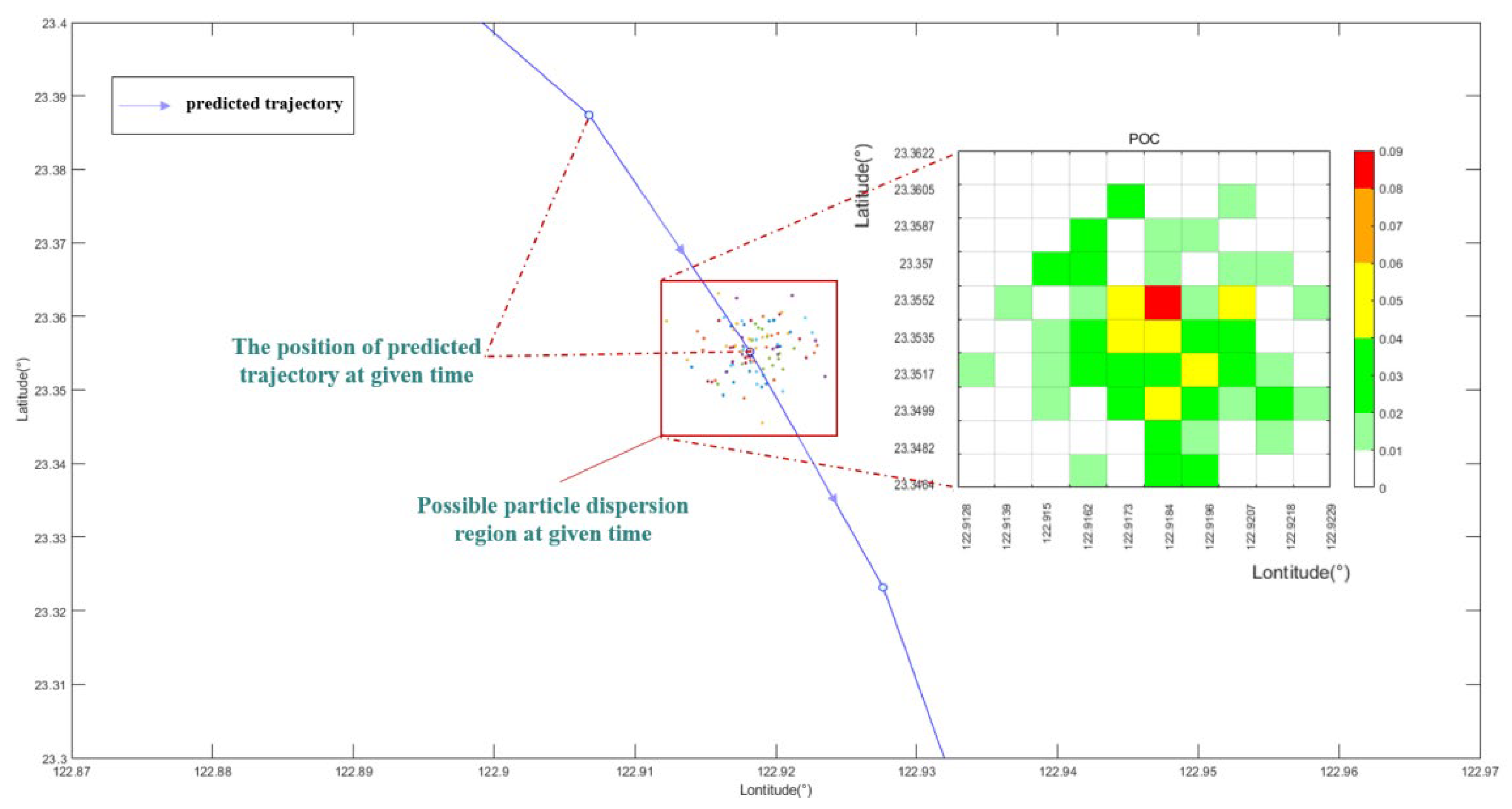
• Based on the proposed FCNN embedding drifting trajectory prediction and correction model for unmanned maritime equipment, the obtained POC for the unmanned maritime equipment SAR region show a significant improvement in accuracy compared to the traditional methods.

2. Methodology

As shown in Figure 1, the method for the prediction and dynamic correction of drifting trajectory for unmanned maritime equipment is divided into two steps. Firstly, based on the weights and the influence of the actual ocean dynamics factors, several primary models are linked to derive the maritime SAR target drifting model. On the basis of the predicted drifting trajectory, the FCNN is introduced to fuse the return signals to fine tune the trajectory parameters in real time. Based on the experiments of unmanned equipment drifting at sea and the actual data obtained, the effect of single-point and multi-point signal return on trajectory correction is analyzed and discussed in real SAR situations. Secondly, based on the corrected trajectory parameters, the POC of an SAR target at a given time is quantified in order to determine the SAR region under the marine environment raster at that moment in time (Figure 1).

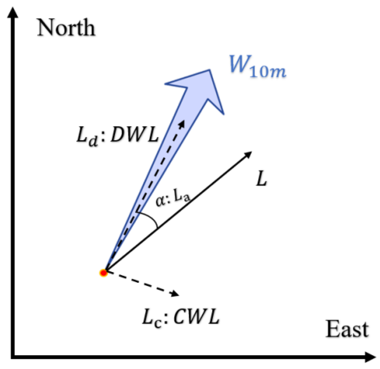
2.1. Unmanned Maritime Equipment Drifting Model

For the analysis of the motion force of the equipment drifting at sea, the underwater part of the target is mainly affected by the ocean surface current and waves while the above-water part is mainly affected by the wind during drifting. Therefore, the SAR target drifting velocity $\mathit{v}$ can be approximated as follows:

$$\mathit{v}={\mathit{v}}_{\mathit{F}-\mathit{s}\mathit{u}\mathit{r}\mathit{f}\mathit{a}\mathit{c}\mathit{e}-\mathit{c}\mathit{u}\mathit{r}\mathit{r}\mathit{e}\mathit{n}\mathit{t}}+\mathit{l}+{\mathit{v}}_{\mathit{F}-\mathit{w}\mathit{a}\mathit{v}\mathit{e}}$$

(1)

In Formula (1), ${\mathit{v}}_{\mathit{F}-\mathit{s}\mathit{u}\mathit{r}\mathit{f}\mathit{a}\mathit{c}\mathit{e}-\mathit{c}\mathit{u}\mathit{r}\mathit{r}\mathit{e}\mathit{n}\mathit{t}}$, $\mathit{l}$, and ${\mathit{v}}_{\mathit{F}-\mathit{w}\mathit{a}\mathit{v}\mathit{e}}$ are the drifting velocities due to ocean current, wind, and wave factors, respectively.

Since the size of unmanned maritime equipment is less than 30 m in length, which is much smaller than the action size of the wave-induced drifting model, it is approximated as having no effect. Therefore, the model can be mainly divided into an ocean-current-induced drifting model and wind-induced drifting model based on the improved LEEWAY model. These two independent models are combined in Formula (1), based on the weights and the influence of actual ocean dynamics factors, to construct the maritime target drifting model. The weights and empirical coefficients related to the actual ocean dynamics are derived from the International Aviation and Maritime Search and Rescue Manual [10] and the National Maritime Search and Rescue Environmental Support Platform.

Since the ocean current in the surface layer of the sea water has the main effect on the drift of the target in distress at sea, so the formula of ocean-current-induced drifting velocity is expressed as follows:

$${\mathit{v}}_{\mathit{F}-\mathit{s}\mathit{u}\mathit{r}\mathit{f}\mathit{a}\mathit{c}\mathit{e}-\mathit{c}\mathit{u}\mathit{r}\mathit{r}\mathit{e}\mathit{n}\mathit{t}}=\lambda ·{\mathit{v}}_{\mathit{s}\mathit{u}\mathit{r}\mathit{f}\mathit{a}\mathit{c}\mathit{e}-\mathit{c}\mathit{u}\mathit{r}\mathit{r}\mathit{e}\mathit{n}\mathit{t}}$$

(2)

In Formula (2), ${\mathit{v}}_{\mathit{s}\mathit{u}\mathit{r}\mathit{f}\mathit{a}\mathit{c}\mathit{e}-\mathit{c}\mathit{u}\mathit{r}\mathit{r}\mathit{e}\mathit{n}\mathit{t}}$ denotes ocean current velocity and $\lambda$ denotes the ocean-current-induced drifting coefficient.

According to the investigated drifting models, the ocean-current-induced drifting velocity is usually assumed to be approximately equal to the surface velocity of the sea water [1], and experiments carried out by scholars have demonstrated that the coefficient of ocean-current-induced drift is approximately 1.2 [11,12].

Wind-induced drift is the movement of an object relative to the surrounding currents due to the action of the wind on its watery portion. Allen (2005) decomposed wind-induced drifting velocity into the more robust components of the downwind leeway (DWL) and crosswind leeway (CWL). CWL has the same probability of deviating left (−CWL) and right (+CWL). Subsequent scholars have also carried out a large number of wind drifting coefficient determination and application research based on this; the principle of the wind-induced drift model is as follows (Figure 2).

The fit to the wind-induced drifting velocity can be expressed as follows:

$$\left\{\begin{array}{c}{L}_d=a_d{\omega }_{10}+b_d+{ϵ}_d \left(DWL\right)\\ L_{c+}=a_{c+}{\omega }_{10}+b_{c+}+{ϵ}_{c+} \left(+CWL\right)\\ L_{c-}=a_{c-}{\omega }_{10}+b_{c-}+{ϵ}_{c-} \left(-CWL\right)\end{array}\right.$$

(3)

$L$ is the wind-induced drifting velocity, $a$ and $b$ are the fitting coefficients, $ϵ$ is the fitting standard deviation, and the subscripts $d$, $c+$, and $c-$ correspond to the directions of the downwind, rightward, and leftward winds, respectively; ${\omega }_{10}$ is the wind speed at 10 m height of the sea surface.

Let $\mathit{s}$ be the velocity vector of the surface current and $\mathit{l}$ be the wind-induced drifting velocity vector of the unmanned maritime equipment, so the drifting velocity vector $\mathit{v}$ of the target can be expressed as

$$\mathit{v}=\mathit{s}+\mathit{l}$$

(4)

Then, the target drifting model can be expressed as

$$X\left(t\right)-X\left(0\right)={{\displaystyle \int }}_0^t\mathit{v}\left(t^{\prime }\right)d{t}^{\prime }={{\displaystyle \int }}_0^t\left[\mathit{s}\left(t^{\prime }\right)+\mathit{l}\left(t^{\prime }\right)\right]d{t}^{\prime }$$

(5)

$X\left(t\right)$ is the position of the unmanned maritime equipment at moment $\mathrm{t}$.

When calculating the displacement of the target, the wind field and ocean current field velocity are decomposed along the direction of longitude and latitude. Based on the velocities, u and v in the corresponding direction are calculated to obtain the drift displacement of the target in distress.

The ocean current field drift calculation formula is tabulated as follows:

$$\left\{\begin{array}{c}dX:U_{wa}=\left(\alpha \cdot \left|U_{wa-lot}\right|+{\rho }_{wa}\cdot cos\left({\theta }_{wa}\right)\right)\\ dY:V_{wa}=\left(\alpha \cdot \left|V_{wa-lat}\right|+{\rho }_{wa}\cdot sin\left({\theta }_{wa}\right)\right)\end{array}\right.$$

(6)

In Formula (6), $U_{wa}$ and $V_{wa}$ denote the ocean-current-induced drifting velocities of the distress target along the longitude and latitude directions, respectively. $\alpha$ is the ocean current field coefficient. $U_{wa-lot}$ and $V_{wa-lat}$ are the velocities of the ocean current along the longitude and latitude directions obtained by the extraction, respectively. ${\rho }_{wa}$ is the ocean current perturbation coefficient, and ${\theta }_{wa}=$ arctan($V_{wa-lat}$/$U_{wa-lot}$) denotes the ocean current angle.

The wind field drift calculation formula is expressed as follows:

$$\left\{\begin{array}{c}dX:U_{wi}=\left(\beta \cdot \left|U_{wi-lot}\right|+{\rho }_{wi}\cdot cos\left({\theta }_{wi}\right)\right)\\ dY:V_{wi}=\left(\beta \cdot \left|V_{wi-lat}\right|+{\rho }_{wi}\cdot sin\left({\theta }_{wi}\right)\right)\end{array}\right.$$

(7)

In Formula (7), $U_{wi}$ and $V_{wi}$ denote the wind-induced drifting velocities of the distress target along the longitude and latitude directions, respectively. β is the wind pressure field coefficient. $U_{wi-lot}$ and $V_{wi-lat}$ denote the wind field velocities along the longitude and latitude directions obtained by extraction, respectively. ${\rho }_{wi}$ is the wind pressure perturbation coefficient, and ${\theta }_{wi}=$ arctan($V_{wi-lat}$/$U_{wi-lot}$) denotes the wind field angle.

The distress target drift consists of two drifts—the ocean current field and the wind field—so the distress target drift calculation formula is expressed as follows:

$$\left\{\begin{array}{c}DX=\left(U_{wi}+U_{wa}\right)\cdot t\\ DY=\left(V_{wi}+V_{wa}\right)\cdot t\end{array}\right.$$

(8)

In Formula (8), $DX$ and $DY$ denote the displacements along the longitude and latitude directions, respectively. $U_{wa}$ and $U_{wi}$ denote the ocean-current-induced and wind-induced drifting velocities along the longitude direction. $V_{wa}$ and $V_{wi}$ denote the ocean-current-induced and wind-induced drifting velocities along the latitude direction. And t is the time interval. Substituting Formulas (6) and (7) yields the following:

$$\left\{\begin{array}{c}DX=\left(\beta \cdot \left|U_{wi-lot}\right|+{\rho }_{wi}\cdot cos{\theta }_{wi}+\alpha \cdot \left|U_{wa-lot}\right|+{\rho }_{wa}\cdot cos{\theta }_{wa}\right)\cdot t\\ DY=\left(\beta \cdot \left|V_{wi-lat}\right|+{\rho }_{wi}\cdot sin{\theta }_{wi}+\alpha \cdot \left|V_{wa-lat}\right|+{\rho }_{wa}\cdot sin{\theta }_{wa}\right)\cdot t\end{array}\right.$$

(9)

At the same time, due to the complexity of the marine environment, the power field information may also have errors. The target drifting process is perturbed by random uncertainty, and the final position has uncertainty. Therefore, this paper adopts the following method: deploying a large number of particles for drifting trajectory prediction and taking the geometric center as the actual predicted trajectory according to the scattering to reduce the influence of such errors, as shown in Section 2.3.

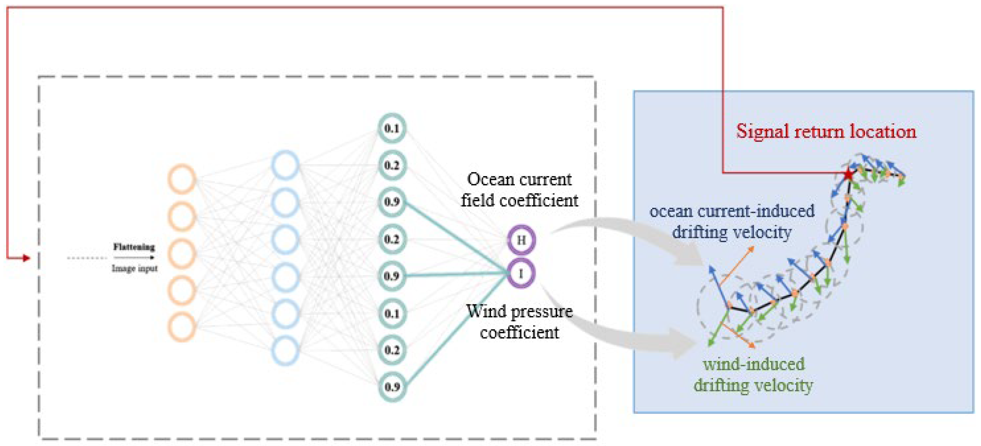
2.2. Trajectory Dynamic Correction Algorithm Based on FCNN

When the unmanned maritime equipment drifts in an unpowered state, the actual trajectory correction cannot be realized by manipulating the equipment’s own power system. However, some strategies can be adopted to correct the predicted trajectory of the unmanned maritime equipment. On the basis of the original drift prediction trajectory and the SAR region, the intermittent positional feedback from the unmanned maritime equipment in the drifting state can be fully utilized to correct the predicted trajectory with its own localization information. This study adopts the intelligent prediction of drift trajectory based on the fully connected neural network (FCNN) embedded method for more accurate trajectory prediction and real-time correction [13].

The neural network used in this paper is a 3-layer network, and the weights are set according to the schematic diagram shown Figure 3.

The output of the i-th hidden layer is obtained after the function’s weighted transformation as follows:

$$g_i=f\left({\omega }_i{g}_{i-1}+b_i\right)$$

(10)

$f$ is the activation function of the hidden layer. $g_{i-1}$ is the input data of the previous layer. The transfer function used in the FCNN designed in this paper is the Sigmoid function. The multilayer perceptron (MLP) network is used in the sensitivity analysis applied in the actual analysis and calculation [14]. Through the sensitivity analysis, the sensitivity parameters that have a greater impact on the total effectiveness index are obtained. And then, the important indexes that affect the effectiveness of the trajectory correction are obtained to analyze the degree of influence on the trajectory correction quantitatively.

By using the accuracy assessment method based on the offset value, the prediction accuracy of the model can be quantitatively assessed. For implementation, the actual value and the predicted value of the model are first obtained from the test set, and for each sample, the distance between the actual value and the predicted value is calculated using the Euclidean distance formula.

$$\rho =\sqrt{{\left({\widehat{x}}_t-x_t\right)}^2+{\left({\widehat{y}}_t-y_t\right)}^2}$$

(11)

The calculation formula is shown in Formula (11). ($x_t$, $y_t$) are the actual coordinates at time $t$, and (${\widehat{x}}_t$, ${\widehat{y}}_t$) are the corresponding corrected coordinates. The accuracy assessment judgment index is derived, as shown in Formula (12):

$$g\left(x_t,y_t,t,\alpha ,\beta \right)={\left(f\left(\alpha ,\beta ,t\right),-\left(x_t,y_t\right)\right)}^2$$

(12)

$f\left(\alpha ,\beta ,t\right)$ is the route prediction or correction model. $\left(x_t,y_t\right)$ are the latitude and longitude positions fed back by the navigator in real time. t is the target drift moment. $\alpha$ and $\beta$ are the ocean current field coefficient and the wind pressure coefficient, respectively. The minimization function $g\left(x_t,y_t,t,\alpha ,\beta \right)$ should be used as the judging index for accuracy assessment.

Therefore, it can be designed as a suitable loss function to measure the gap between the parameters predicted by the neural network and the real optimal parameters. And the mean-squared error (MSE) loss function is selected [15]. This form is more sensitive to error and is computationally easier to derive and optimize. The loss function is obtained as follows:

$$L\left(\alpha ,\beta \right)={\displaystyle \frac{1}{N}}{\displaystyle \sum }_{t=1}^N\left[{\left({\widehat{x}}_t-x_t\right)}^2+{\left({\widehat{y}}_t-y_t\right)}^2\right]$$

(13)

In Formula (13), N is the number of time steps. ($x_t$, $y_t$) are the actual coordinates of the target at time $t$. (${\widehat{x}}_t$, ${\widehat{y}}_t$) are the corresponding corrected coordinates. $L\left(\alpha ,\beta \right)$ is the total loss.

Based on the above loss function and FCNN model settings, the parameter optimization in nested loops is performed to achieve the predicted trajectory parameters with minimum loss.

$$\theta \left({\alpha }^{*},{\beta }^{*}\right)=arg\underset{\theta }{min}L\left(F\left(X;\omega \right),{\theta }_{true}\right)$$

(14)

$\theta \left({\alpha }^{*},{\beta }^{*}\right)$ denotes the learned optimal ocean current field coefficient and wind pressure coefficient. $F\left(X;\omega \right)$ is the function of FCNN that receives the input features $X$, and it is defined by the parameter $\omega$. $L$ is the loss function that measures the difference between the neural network outputs and the optimal parameter ${\theta }_{true}$, $argmin$ denotes the search to minimize the loss function by the parameter values, and the $X$ is the feature vector.

Substituting the parameters obtained after the optimization search into Formula (9), the parameters of the original predicted trajectory are refined and replaced, and the modified trajectory drifting model can be obtained:

$$\left\{\begin{array}{c}DX=\left({\beta }^{*}\cdot \left|U_{wi-lot}\right|+{\rho }_{wi}\cdot cos{\theta }_{wi}+{\alpha }^{*}\cdot \left|U_{wa-lot}\right|+{\rho }_{wa}\cdot cos{\theta }_{wa}\right)\cdot t\\ DY=\left({\beta }^{*}\cdot \left|V_{wi-lat}\right|+{\rho }_{wi}\cdot sin{\theta }_{wi}+{\alpha }^{*}\cdot \left|V_{wa-lat}\right|+{\rho }_{wa}\cdot sin{\theta }_{wa}\right)\cdot t\end{array}\right.$$

(15)

In Formula (15), $DX$ and $DY$ denote the displacements along the longitude and latitude directions. ${\alpha }^{*}$ denotes the corrected ocean current field coefficient. ${\beta }^{*}$ denotes the corrected wind pressure coefficient.

2.3. Monte Carlo Simulation-Based Quantification of the POC in SAR Region

In practice, due to the irregular geometry of the target, the complexity of the marine environment and the possible errors in the power field information, there is uncertainty in the final position of the target [16]. Therefore, the decision-making information given by the maritime SAR prediction is not only the trajectory but also the SAR region. Based on the real-time corrected SAR target trajectory parameters, Monte Carlo simulation is used to quantify the POC of the SAR target under the marine environment.

The unmanned maritime equipment is abstracted as a random particle through particle simulation. The position of the particle at the moment $t_0$ is known, and its position at $t_0$ is independent of the position of the particle before $t_0$. The “posteriority-free” process can be described by the Markov process. The process of a particle drifting in the sea can be expressed as follows:

$$P(X_{t+1}|X_t,X_{t-1},X_{t-2},\dots ,X_1)=P(X_{t+1}|X_t)$$

(16)

$P$ is the conditional distribution function, and $X$ is a Markov variable. Formula (16) states that the position of the particle at moment $t$ during the drift process is a known condition, and the position at the moment $t+1$ is independent of the position before the moment $t$. The particle drift satisfies the differential equation [17]:

$$\left\{\begin{array}{c}\mathit{d}\mathit{X}=\mathit{V}\left(\mathit{X},\mathit{t}\right)\mathit{d}\mathit{t}+\mathit{d}{\mathit{X}}^{\prime }\\ \mathit{d}{\mathit{X}}^{\prime }={\mathit{K}}^{{\displaystyle \frac{\mathbf{1}}{\mathbf{2}}}}\mathit{d}\mathit{w}\end{array}\right.$$

(17)

$\mathit{d}\mathit{X}$ is the displacement of the particle in the dt time period. V is the particle mean drifting velocity function, which is affected by the marine environment, meteorological data, and the drifting attributes of the equipment represented by the particle. $\mathit{d}{\mathit{X}}^{\prime }$ is random perturbation, which represents the perturbed displacement caused by the error of the wind pressure, the marine environment, and the meteorological data in the $\mathit{d}\mathit{t}$ time period. $\mathit{d}\mathit{w}\left(\mathit{t}\right)$ is a stochastic increment which obeys a normal distribution with the mechanism variance and mean. K is the perturbation diffusion coefficient, which is expressed as follows:

$$K={\sigma }_v^{2}T$$

(18)

${\sigma }_v^2$ is the variance in the perturbed velocity field (wind pressure and ocean surface current velocity), and $T$ is the perturbation time.

Next, the Monte Carlo method is used for calculating the search region. A large number of particles are deployed to drift, with each particle representing a possible location of unmanned maritime equipment. Using the Monte Carlo simulation method, random uncertainty perturbations are superimposed on the theoretical predicted trajectories to simulate the impact of uncertain factors in the marine environment, thereby simulating and calculating the potential actual trajectories of the particles. After each iteration, the particle distribution is obtained at a specific moment. Calculations were performed on the dataset of particle distributions at the same moment, where the geometric center of the particle distribution area serves as the center of the SAR region and the SAR region is regarded as circle-like. See Figure 4.

Using the drifting distances obtained from the model of drifting trajectory prediction, the following formula is established:

$$\left\{\begin{array}{c}{D}_{initial}={\lambda }_0·S_e\\ L=\sqrt{D_x^2+D_y^2}\\ D_{next}={\displaystyle \frac{L}{{\lambda }_1}}+D_{initial}\end{array}\right.$$

(19)

In Formula (19), $D_{initial}$ and $D_{next}$ denote the initial state value of particle dispersion and the state at the next moment, respectively. ${\lambda }_0$, ${\lambda }_1$, and $S_e$ are empirical coefficients. ${\lambda }_0·S_e$ represents the distribution of particles in the initial state (initial position error). $S_e$ indicates a normal distribution. ${\lambda }_0$ denotes the magnitude of the initial position error [18]. The error range coefficient ${\lambda }_1$ is used to constrain the growth size of the SAR region with each iteration update, to control the error range. Its role is to ensure that the particles distributed within the SAR region meet a 95% confidence interval relative to the total number of particles. The model calculates the SAR region of a series of waypoint prediction points of the distress target; the $D_{next}$ of the previous moment is the $D_{initial}$ of the next moment.

During calculations, the positions of particles at the same moment in time are evaluated. If a particle is within the search and rescue region at this moment, it is considered as an effective particle for subsequent POC calculations. If a particle is outside the SAR region at this moment, it is deemed as an ineffective particle and needs to be removed to prevent inaccuracies in the POC calculation results due to the inclusion of ineffective particles.

Finally, the particle distribution at that moment is counted, and the maximum and minimum values of the latitude and longitude of the discrete points at that moment are selected as the basis of division. The side length X of the SAR region A is the max–min difference in longitude, and the side length Y is the max–min difference in latitude in the set of discrete points at that moment. The SAR region $\mathit{A}$ is uniformly divided into $Lx$×$Ly$ grids according to its length. With each grid serving as a subregion, the number of particles in each subregion is counted to obtain the particle distribution matrix $\mathit{A}$.

$$\mathit{A}\left(i,j\right)=n_{ij}, 0\le i\le Lx,0\le j\le Ly$$

(20)

$n_{ij}$ denotes the number of subregion particles in the i-th row and j-th column.

$$\mathit{P}\mathit{O}{\mathit{C}}_{\mathit{i}\mathit{j}}={\displaystyle \frac{n_{ij}}{{{\displaystyle \sum }}_{i=1,j=1}^{LxLy}\mathit{A}\left(i,j\right)}}$$

(21)

According to Formula (21), the matrix $\mathit{A}$ is normalized to obtain the distribution matrix of the POC, which achieves the uncertainty quantification of the SAR region.

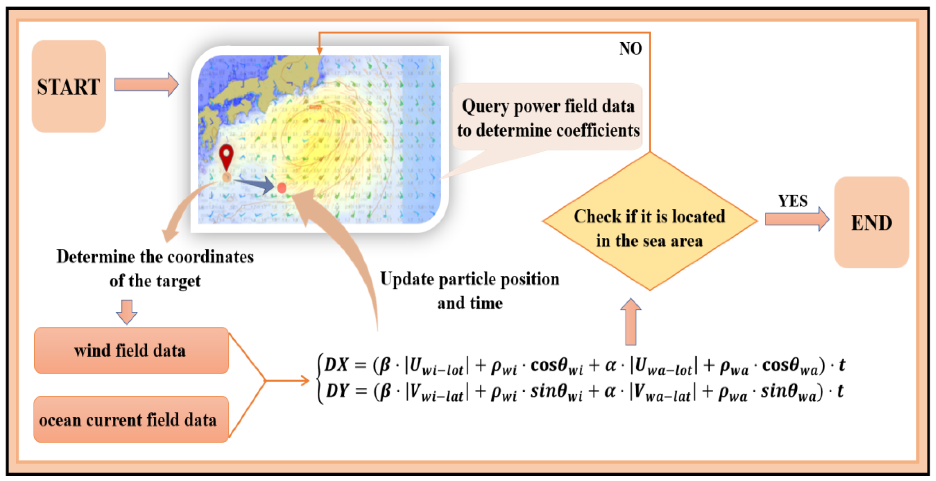
2.4. Steps for Predicting Target Drift Trajectory

According to the established drifting motion model of the target, substituting Formula (5) into the differential equation of the particle’s drifting trajectory, Formula (17) yields the following:

$$\left\{\begin{array}{c}\mathit{d}\mathit{X}=\mathit{V}\left(\mathit{X},\mathit{t}\right)\mathit{d}\mathit{t}+\mathit{d}{\mathit{X}}^{\prime }\\ \mathit{d}{\mathit{X}}^{\prime }={\left({\displaystyle \frac{{\sigma }_{\mathit{v}}^{\mathbf{2}}\mathit{d}\mathit{t}}{\mathbf{2}}}\right)}^{\mathbf{1}\mathbf{/}\mathbf{2}}\mathit{d}\mathit{w}\end{array}\right.$$

(22)

Discretizing Formula (22) to obtain the numerical equation for the particle drift trajectory results in the following:

$$\left\{\begin{array}{c}{\mathit{X}}_{\mathit{i}+\mathbf{1},\mathit{j}+\mathbf{1}}^{\mathit{n}+\mathbf{1}}={\mathit{X}}_{\mathit{i},\mathit{j}}^{\mathit{n}}+{\mathit{V}}_{\mathit{i},\mathit{j}}^{\mathit{n}}\Delta \mathit{t}+\Delta {\mathit{X}}^{\prime \mathit{n}}\\ \Delta {\mathit{X}}^{\prime \mathit{n}}={\left({\displaystyle \frac{{\sigma }_{\mathit{v}}^{\mathbf{2}}\mathit{d}\mathit{t}}{\mathbf{2}}}\right)}^{\mathbf{1}/\mathbf{2}}{\mathit{w}}^{\mathit{n}}\end{array}\right.$$

(23)

$\Delta t$ is the drift projection time step. ${\mathit{X}}_{\mathit{i}+\mathbf{1},\mathit{j}+\mathbf{1}}^{\mathit{n}+\mathbf{1}}$ denotes the position of the particle after the completion of the n-th projection. ${\mathit{V}}_{\mathit{i},\mathit{j}}^{\mathit{n}}$ denotes the average velocity of the particle at position ${\mathit{X}}_{\mathit{i},\mathit{j}}^{\mathit{n}}$ during the n-th projection. It is the perturbation displacement within step $\Delta t$ in the n-th projection, which is known as the projected displacement within the time step. ${\mathit{\sigma }}_{\mathit{v}}^{\mathit{2}}$ is the variance in the perturbed velocity field, which is a reflection of the combination of wind pressure perturbations and ocean current field perturbations. ${\mathit{w}}^{\mathit{n}}$ is a random variable.

Over time, the particles are constantly moving, driven by the wind and flow fields, and the steps that lead to the prediction of the particle drifting trajectory are shown in Figure 5.

3. Experiments

3.1. Data Preparation

The ocean hydrological data used in this paper originate from the FIOCOM reanalysis data developed by the First Institute of Oceanography of the Ministry of Natural Resources [19]. This dataset integrates the coupled models of ocean waves, tidal currents, and circulation. And it uses ocean dynamics models and data assimilation to integrate and analyze the historical observational data to produce high-quality data products. FIOCOM covers 3D ocean current dynamics, wave characteristics, surface wind field status, sound speed, and other key ocean environmental parameters. It provides a full range of information resources for this study and meets the data needs for the target trajectory prediction in this paper. The time period for the analysis of the multidimensional marine environmental data in this paper was selected as 1 January 2023 to 31 December 2023, and the spatial area was selected as the sea area from 105° to 160° east longitude and from 0° to 41° north latitude.

According to the model constructed in this paper, the main data used were the ocean current field and wind field data. Maritime SAR research generally takes the wind speed at a 10 m height from the sea surface and the current speed at a water depth of 0.5 m to make ocean power projections [9]. Therefore, we process these two parts of data before the prediction of the drift trajectory of unmanned equipment.

In the ocean current field data processing stage, the grid distribution information of the longitudinal, latitudinal, time series, and ocean current field depth direction data are read to calculate the ocean current velocities of the east–west component and north–south component.

In the wind field data processing stage, the longitudinal and latitudinal grids as well as the time series data in the wind field data are read to calculate the wind field velocities of the east–west component and the north–south component.

Since the acquired wind field and current field data are discrete data, in order to increase the accuracy of the route prediction, this paper interpolates the discrete marine environmental data and uses the current field and wind field data obtained at the end of the processing for the unmanned maritime equipment drift trajectory computation, improving the resolution to be accurate to the minute level and providing feasible data for the subsequent calculations of uncertainty quantification in the SAR region and other related computations.

In order to validate the model and trajectory correction method of this paper, six sets of unmanned maritime equipment were successively deployed along the southwest of Penghu Islands in April 2023, respectively, PO1~PO6, to carry out the validation experiments of the prediction of drifting trajectory and the refinement of intelligent correction of drift trajectory parameters.

Through the experiment, the natural drift trajectory data of the target without its own power are obtained. In this paper, a total of 104 equipment unpowered drift datapoints generated by the waterborne data platform in different time periods are selected as test data.

The data are preprocessed and cleaned, and the latitude and longitude position data of the target and the corresponding time series, wind field data, ocean current field data and other information on the region are extracted from

Table 1. Data table format for this article.

Lon_1	Lat_1	t_1	Lon_2	Lat_2	t_2	…	Lon_n	Lat_n	t_n	Wind_c	Water_c
119.38° E	22.97° N	…	119.40° E	22.95° N	…	…	119.68° E	22.66° N	…	0.0405	1.0431
122.47° E	21.61° N	…	122.49° E	21.58° N	…	…	124.17° E	19.67° N	…	0.0485	1.4819
…	…	…	…	…	…	…	…	…	…	…	…
124.91° E	22.08° N	…	124.92° E	22.07° N	…	…	125.20° E	22.04° N	…	0.0370	1.1100

as input data, and the last two columns represent the parameters to be fitted.

The purpose of the data cleaning process is to extract useful features and prepare data for the training and validation of the trajectory correction model. Based on the latitude and longitude information of the start and target points, displacements and associated features are calculated. These features can be used as inputs to the model for predicting unpowered drift trajectory corrections.

After training, the trained network is saved. The model’s performance is verified by testing through the already-trained artificial neural network using pre-divided data as a test set, and the verified model is applied to the actual unmanned aerial vehicle drifting trajectory correction task.

3.2. Model Parameter Setting and Initialization

The main parameters of the basic model used in this paper are shown in

Table 2. Equipment initialization data for single-point position information return.

Data Date	Starting Moment	Prediction Interval (min)	Projected Length (h)	Latitude and Longitude of the Starting Point
22 April 2023	12:00:00	5	24	(122.5° E, 23.7° N)

and

Table 3. Unmanned maritime equipment drifting parameters.

Equipment Drifting Parameters	Data
Wind pressure coefficient (×10−2)	4.00
Wind pressure perturbation coefficient	0.16
Ocean current field coefficient	1.20
Ocean current perturbation coefficient	0.25

.

Meanwhile, in the experiment of fine correction of trajectory parameters of multi-point position information return, after model construction and model training, a section of trajectory of PO1 is selected as the object of experimental verification. The initial data are shown in

Table 4. Experimental data for multi-point position information return.

Equipment Type	Data Date	Predicting the Starting Moment	Projected Length (h)	Latitude and Longitude of the Starting Point
PO1	22 April 2023	12:11:39	24	(119.4662° E, 22.3588° N)

.

3.3. Model Training

The loss variation during training and the post-training prediction trajectory correction results are as follows (Figure 6).

As shown in Figure 7, the loss value reaches convergence quickly after more than 20 training sessions and fluctuates within a small range. The statistically obtained minimum loss value is 0.0979. The final wind pressure coefficients and ocean current field coefficients are closer to the actual parameters. There is no overfitting phenomenon, so the established model fits well with the modified actual needs.

3.4. Evaluation Criteria

In order to evaluate the effect of the corrected predicted trajectories, the Sum-of-Pairs Distance (SPD) method is adopted as a judgement criterion for the similarity metric between the corrected trajectories and the corresponding actual trajectories [20]. We calculate the difference in Euclidean distance between the target predicted and actual points of the same time series and average the calculation after summing the distance difference to obtain the average error offset distance.

$$dSPD\left(T_1,T_2\right)={\displaystyle \sum }_{p_1\in T_1}{\displaystyle \sum }_{p_2\in T_2}\Vert p_1-p_2\Vert$$

(24)

$${\delta }_{off}=dSPD\left(T_1,T_2\right)/n$$

(25)

In the above equation, $T_1$ and $T_2$ denote two trajectories, each trajectory containing n coordinate points. $\Vert p_1-p_2\Vert$ represents the Euclidean distance of the corresponding points on the first trajectory and the second trajectory. ${\delta }_{off}$ is the average error offset distance.

4. Results and Discussions

4.1. Trajectory Correction Based on Single-Point Position Information Returns and Discussion

The test results of the trajectory correction after single-point real position information return are given below. Based on this signal information, the parameters of the original predicted trajectory are corrected more finely in real time, and then, the trajectory correction is realized.

As shown in

Table 5. Comparison of parameters after trajectory correction.

Equipment Drifting Parameters	Predicted Parameters	Corrected Parameters
Wind pressure coefficient (×10−2)	4.00	3.85
Ocean current field coefficient	1.20	1.1575

, the data in the first column are the values of the predicted trajectory parameters obtained empirically from the literature. The unmanned maritime equipment returned one signal when it was located at (122.8039° E, 23.5109° N). The second column of data shows the final result of the parameter refinement correction of the FCNN output return on the basis of this signal.

As shown in Figure 8, after the target returned the signal of position information once at the coordinates (122.8039° E, 23.5109° N) at 13:30, the neural network corrected the original predicted trajectory and then outputted the corrected trajectory that was closer to the actual movement of the target. It can be seen that at the return point, the actual target has already deviated from the predicted trajectory at the expected time due to its own attribute characteristics and the influence of uncertain variables in the drift process. The corrected trajectory of the target, which better matches the actual drifting trajectory, is obtained by the accurate correction of the artificial neural network after the fusion of the returned information, thus improving the search efficiency.

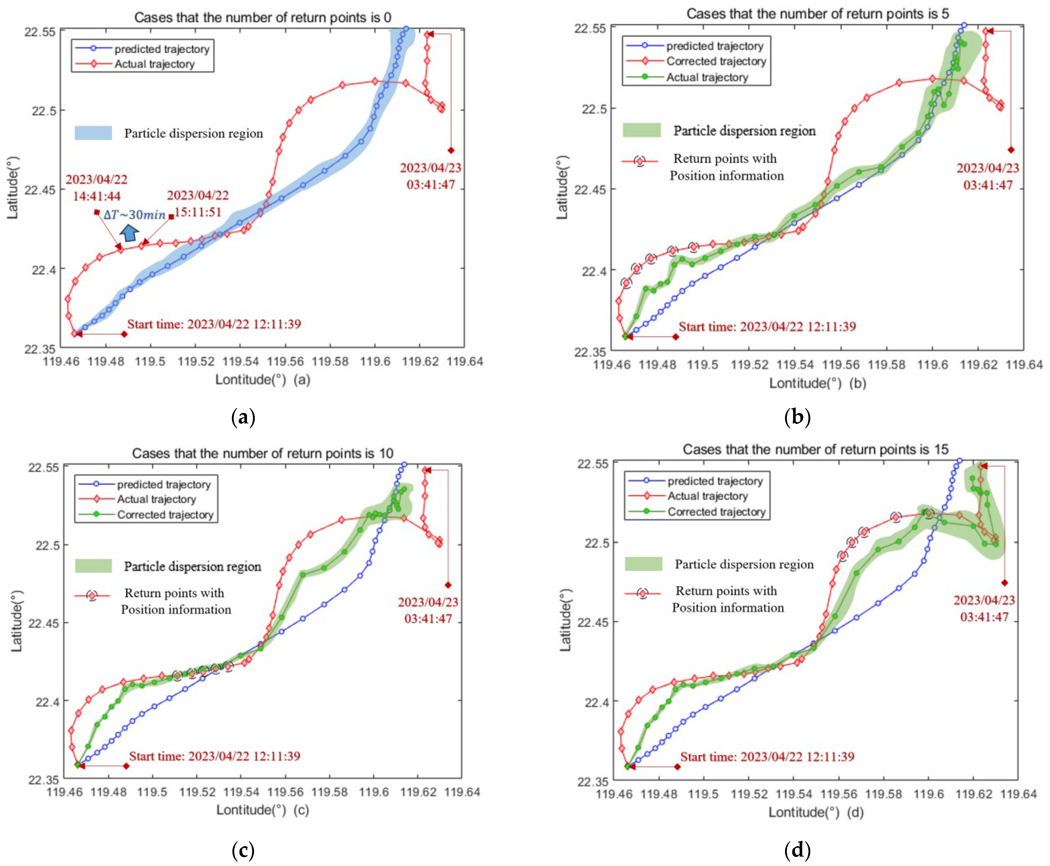
4.2. Trajectory Correction Based on Multi-Point Position Information Returns and Discussion

The FCNN trajectory intelligence correction methodology designed in this paper can learn from multiple returned GPS locations to correct predicted drift trajectories in real time. Every time a signal is returned, the parameters of the trajectory in the interval between the two signals are refined and re-corrected. Being closely adapted to the real search and rescue environment, as the number of target feedback points increases, the system carries out real-time updating and correction of trajectory realization.

In the experiment of this study, the unmanned equipment actually returns self-location information about every half an hour. In the early stage of the experimental design, we conducted a pre-experiment and compared the effect of trajectory corrections under different frequencies. It can be found that the correction effect is positively correlated with the number of information returns, and the total trajectory correction of every five signal returns is more representative. The correction effect is also more obvious and intuitive. Therefore, a 2 h correction cycle was chosen for the experiment while corrections and comparisons were made every five signal transmissions.

In order to verify the effectiveness of the intelligent correction model of this paper for the fusion of the multiple-return information, according to the drift trajectory data of unmanned maritime equipment collected during sea trial experiments, take part of the trajectory of PO1 as an example—the neural network was given 0, 5, 10, and 15 input signal points, respectively—to compare the effect of trajectory correction based on different numbers of points. Observe the comparison of the original predicted SAR trajectory, the actual motion point trajectory, and the real-time corrected re-feedback accurate trajectory, as shown in the figure below.

According to Formula (23), the average error offset distance between the geometric center of the corrected trajectory and the actual trajectory for the same time series after different numbers of return points is obtained as follows:

Table 6. The error magnitude affected by the number of correction points in time series.

Number of Return Points	Feedback Time for Position Information	Distance of Average Offset (km)
0	\	5.75
1	22 April 2023 13:41:45	5.17
2	22 April 2023 14:11:38	4.92
3	22 April 2023 14:41:44	4.69
4	22 April 2023 15:11:51	4.34
5	22 April 2023 15:41:45	3.94

shows how the error magnitude is affected by the number of correction points with time series (take the example of returning five points), and

Table 7. Comparison of trajectory correction.

Number of Return Points	Predicted Value (Wind Pressure Coefficient (×10−2), Ocean Current Field Coefficient)	Corrected Value (Wind Pressure Coefficient (×10−2), Ocean Current Field Coefficient)	Distance of Average Offset (km)
0	(4.00, 1.2000)	\	5.75
5	(4.00, 1.2000)	(3.87, 1.2595)	3.94
10	(4.00, 1.2000)	(3.53, 1.2351)	1.11
15	(4.00, 1.2000)	(4.35, 1.2384)	4.11 × 10−1

focuses on demonstrating the effects of multi-point corrections.

Figure 9a–d represent the effect of the model’s correction on the predicted target drift trajectory after returning different numbers of points and the comparison of the corrected trajectory with the actual drift, respectively. The blue trajectory is the original predicted trajectory, and the blue area is the resulting particle dispersal containment area. The red trajectory is the target actual motion trajectory. The green trajectory is the corrected trajectory. To overcome the effects of the complexity of the marine environment, a large number of particles are dispersed for drift. The geometric center of the dispersal region is set as the trajectory point trace, and the green area is the resulting particle dispersal containment area.

As can be seen from Figure 9a,b, after the parameter correction of the returned signal from the unmanned maritime equipment, the fitted re-corrected trajectory fits the actual trajectory better than the original predicted trajectory, which plays the role of narrowing the error and increasing the efficiency of search and rescue.

With the extension of time, the later drift prediction requires more accurate real-time correction to make the predicted trajectory parameters more convergent with the actual motion parameters. Comparing the corrected trajectories with the actual motion trends of the unmanned maritime equipment in Figure 9b–d, it can be seen that as more position signals are returned, the feedback parameter values are more accurate, and the trajectory is closer to the actual trajectory.

According to the particle scattering range in Figure 9d, it can be seen that after the prediction was carried out for 18 h to back-propagate the 15-point signal, the actual point trajectory is included in the possible range of the corrected trajectory, i.e., the corrected trajectory has coincided with the actual trajectory. It is also more in line with the process of real-time parameter correction that can be carried out immediately after the capture of target signals in the actual SAR process, and the newly acquired signals can be continuously utilized to make the prediction more accurate, thus improving the efficiency of SAR.

From Figure 9a,d, it can be seen that the particle dispersion region of the corrected trajectory is closer to the actual trajectory than the particle dispersion region of the initial predicted trajectory. It indicates that the POC of the SAR region calculated by the corrected trajectory is more accurate than the POC obtained from the initial predicted trajectory.

It is also intuitively clear from the data in Table 6 and Table 7 that as the number of return points increases, the average error offset distance decreases, and the drift trajectory correction effect is improved. When the number of return points reaches 15, the average error offset distance is reduced from 5.75 km to 4.11$\times {10}^{-1}$ km, which is one order of magnitude lower, and the corrected trajectory is almost the same as the actual one.

Through the returned signal points, the drift trajectory parameters of the unmanned maritime equipment are accurately corrected in real time, and the corrected and more accurate theoretical trajectory is obtained. The redundancy of the original predicted trajectory is reduced, and the scope of search and rescue is more precise. Therefore, it can avoid blindness in the organization of unmanned maritime equipment search and rescue operations and improve the efficiency and effectiveness of search and rescue implementation.

4.3. Quantification of the POC in the SAR Region Based on Corrected Trajectories

According to the constructed discrete model of offshore particle random drift, scattering particles in the initial point area for trajectory prediction drift. Wind and ocean current field error perturbations are imposed during particle drift, and the effects of less weighted uncertainties such as biological factors, wave factors, etc., are taken into account. We adopt the principle of random collisional disruptiveness and count the range of discrete distributions of points at the same moment in time to obtain the search and rescue region at that moment in time, as shown in Figure 10.

The particles obtained from the Monte Carlo simulation are counted, and the data are visualized as heat map output to form the precise search and rescue area at any moment during the drifting process of the unmanned maritime equipment, which provides support for the formulation of search and rescue programs. See Figure 11.

5. Conclusions

In this study, we first establish a drifting trajectory prediction model for unmanned maritime equipment and an SAR region prediction model based on Monte Carlo simulations. In addition, a prediction trajectory correction method is proposed based on the FCNN embedding model. This method can dynamically correct the original predicted trajectory by using the SAR target’s feedback of its own positional information. It significantly improves the prediction accuracy of the drifting trajectory and SAR region. The experimental results show that as more positional points are returned and considered during the SAR process, the more accurate the corrected trajectory achieved is compared with the actual trajectory. The average deviation distances between the predicted and actual trajectories are reduced from 5.75 km to 4.11$\times {10}^{-1}$ km by the proposed FCNN trajectory re-correction method after utilizing a number of position information points. Moreover, the proposed method is found to be efficient, which can support the real-time requirements of dynamic trajectory prediction in maritime SAR scenarios.

5.1. Limitations

The influence of wave actions is not considered in the drifting influence factors for unmanned maritime equipment at sea in this study. However, when the SAR target is large in size and in a non-offshore area, the drifting velocities caused by wave actions will have some non-negligible influence and are positively correlated with the volume of the floating object. Therefore, it may also be one of the important factors affecting the accuracy of the proposed prediction model. Fully considering the effects of additional wave actions generated by the movement of other sailing/drifting objects and swell waves, a finer model can also be built to obtain a more accurate prediction of the drifting trajectory of unmanned maritime equipment. This is also some part of our future work.

5.2. Future Work

When predicting the drifting trajectory, the marine environmental information used is the forecast data, which usually have poor spatial and temporal resolutions and certain errors. The environmental data used for trajectory prediction in this study are actually directly interpolated to improve the spatial and temporal resolutions. However, the direct interpolations of the wind field and ocean current field are not necessarily accurate, which could introduce a certain degree of errors to the trajectory prediction. The usage of more accurate environmental data could improve the prediction accuracy of the trajectory. In addition, uncertain disturbances (e.g., biological disturbances) during the drifting process of the unmanned maritime equipment may also adversely affect the trajectory parameter corrections, which also will be carefully studied in future work.

References

1. Anderson, E.; Odulo, A.; Spaulding, M. Modeling of Leeway Drift; U.S. Coast Guard Research and Development Center: Washington, DC, USA, 1998.
2. Hodgins, D.O.; Hodgins, S.L.M. Phase II Leeway Dynamics Program: Development and Verification of a Mathematical Drift for Liferafts and Small Boats; Canadian Coast Guard: Ottawa, ON, Canada, 1998.
3. Allen, A.; Plourde, J.V. Review of Leeway: Field Experiments and Implementation; U.S. Coast Guard Research and Development Center: Groton, MA, USA, 1999.
4. Allen, A. Leeway Divergence. Leeway Divergence; U.S. Coast Guard Research and Development Center: Washington, DC, USA, 2005.
5. Röhrs, J.; Christensen, K.H.; Hole, L.R.; Broström, G.; Drivdal, M.; Sundby, S. Observation-based evaluation of surface wave effects on currents and trajectory forecasts. Ocean Dyn. 2012, 62, 1519–1533. [Google Scholar] [CrossRef]
6. Xu, J.; Gao, S.; Ge, Y.; Li, R.; Wu, L.-J.; Liu, G. Analysis of Wave Effect on Drifting Trajectory of Float at Sea. J. Inst. Disaster Prev. 2017, 19, 75–79. [Google Scholar]
7. Spaulding, M.L.; Howlett, E. Application of SARMAP to estimate probable search area for objects lost at sea. Mar. Technol. Soc. J. 1996, 30, 17–25. [Google Scholar]
8. Zhu, G.; Mou, L.; Wang, D. Advance in maritime search and rescue decision support techniques. J. Appl. Oceanogr. 2019, 38, 440–449. [Google Scholar]
9. Jiang, H.L.; Sun, Z.C.; Li, L.L.; Liu, B.; Wu, J.P. A Monte Carlo-based model for maritime search area determination. Waterw. Ports 2011, 32, 6. [Google Scholar]
10. International Maritime Organization/International Civil Aviation Organization. International Aviation and Maritime Search and Rescue Manual. Maritime Safety Administration of the People’s Republic of China, Translation; Science Press: Beijing, China, 2005. [Google Scholar]
11. Huang, J.; Xu, J.; Gao, S.; Guo, J. Factors analysis on sea surface drift trajectory forecasting based on field experiment. Mar. Forecast. 2014, 31, 8. [Google Scholar]
12. Zhou, S.; Yang, Y.; Feng, W. Experimental study of sea drift of simulated human and unpowered fishing vessels in Guangdong waters. J. Trop. Oceanogr. 2013, 32, 87–94. [Google Scholar]
13. Wu, W. Neural Network Computing; Higher Education Press: Beijing, China, 2003. [Google Scholar]
14. Zhang, Q. Introduction to Artificial Neural Networks; China Water Resources and Hydropower Press: Beijing, China, 2004. [Google Scholar]
15. Jia, K. Improvement of a Backpropagation Algorithm for Feedforward Neural Networks. Ph.D. Thesis, Dalian University of Technology, Dalian, China, 2011. [Google Scholar]
16. Xiao, F. Research on Key Technologies of Maritime Search and Rescue Decision Support System. Ph.D. Thesis, Dalian Maritime University, Dalian, China, 2011. [Google Scholar]
17. Xiao, F.; Yin, Y.; Jin, Y. Determination of Maritime Search Area Based on Stochastic Particle Simulation. Navig. China 2011, 34, 34–39. [Google Scholar]
18. Jiang, H.-L. Study on Determining Search Area Model for SAR at Sea. Master’s Thesis, Dalian University of Technology, Dalian, China, 2011. [Google Scholar]
19. FIO Coupled Ocean Model. Available online: http://fiocom.fio.org.cn/introduction.html (accessed on 22 April 2023).
20. Li, Y.; Qi, L.; Liang, G. A Ship Trajectory Clustering Method Considering the Spatiotemporal Characteristics of Traffic Flow. J. Wuhan Univ. Technol. 2024, 46, 107–115. [Google Scholar]
Figure 1. The method overview.
Jmse 12 02262 g001
Figure 2. Wind-induced drifting velocity decomposition for LEEWAY model.
Jmse 12 02262 g002
Figure 3. Schematic of the designed FCNN trajectory’s parameter correction.
Jmse 12 02262 g003
Figure 4. Monte Carlo model for target drift motion.
Jmse 12 02262 g004
Figure 5. Steps for predicting target drifting trajectory.
Jmse 12 02262 g005
Figure 6. The actual drifting trajectories of equipment in experiments.
Jmse 12 02262 g006
Figure 7. Artificial neural network model training effect.
Jmse 12 02262 g007
Figure 8. Target drifting trajectory after FCNN correction.
Jmse 12 02262 g008
Figure 9. Trajectory correction of multi-point signal returns (ad).
Jmse 12 02262 g009
Figure 10. Theoretical trajectory and actual search and rescue ranges.
Jmse 12 02262 g010
Figure 11. Visualization of uncertainty quantification in search and rescue region.
Jmse 12 02262 g011