Two-Dimensional Numerical Method for Predicting the Resistance of Ships in Pack Ice: Development and Validation

Abstract

This study presents a 2D numerical simulation method for predicting the resistance of ships navigating in pack ice. The key contribution of this study lies in the derivation of analytical closed-form solutions for calculating the flexural deformation and stress distribution in an elastic plate using Symplectic Mechanics and Hooke’s laws. These solutions are used to determine the failure mode of ice floes. Linear Elastic Fracture Mechanics (LEFMs) and the weight function method are utilized to analyze crack initiation, propagation, and fracture. Ice is broken when a crack propagates to 14.5% of the ice length. The compressive strength of ice and the contact area are used to calculate the ice load. A collision method was developed based on the Sweep and Prune (SAP) and Gilbert–Johnson–Keerthi (GJK) algorithms. A program for predicting the resistance of ships navigating in pack ice was developed based on MATLAB and the aforementioned theories. The navigation resistance of RV Xuelong at different ice concentrations and speeds was simulated and compared with the model test results from an ice tank. The comparison shows that the simulation results are consistent with the test results, with an average error of 9.05%, indicating the effectiveness and reliability of this numerical method. This study lays a solid foundation for future research on autonomous ship navigation in pack ice.

1. Introduction

Global warming has significantly accelerated the melting of polar ice sheets, expanded the navigable regions, and enhanced the commercial viability of polar routes [1]. However, this expansion is accompanied by increased risks. Ice floes have a significant impact on the maneuverability, operational capabilities, and structural safety of ships navigating in these areas [2]. Therefore, it is necessary to investigate the effects of ice floes on ship navigation performance to ensure the safety of maritime operations.

The numerical simulation of the resistance of a ship navigating in pack ice has developed rapidly, which has been driven by advances in computational technology. The Finite Element Method (FEM) and Discrete Element Method (DEM) have been widely applied [3]. Numerous researchers use commercial Computational Fluid Dynamics (CFD) software in conjunction with these methods to carry out simulations. Such integrations have led to the development of combined CFD–FEM and CFD–DEM simulation approaches [4,5,6,7,8]. There are still several challenges in accurately calculating the complex multi-physics of ship–ice phenomena. For example, the main challenge of the Finite Element Method (FEM) is its computational efficiency and accuracy, especially when simulating splitting and complex nonlinear materials. Conversely, the DEM may be inadequate for capturing responses from continuous media, such as the structural behavior of ships. Additionally, these methods often demand significant computational resources and typically rely on high-performance computing platforms, particularly when conducting simulations of full-scale ship–ice collision scenarios. This study attempted to develop a novel high-performance numerical method for simulating ship–ice collision.

This method predicts the resistance of a ship navigating in pack ice based on a semi-theoretical and empirical approach. Theoretically, this method consumes fewer computing resources and improves computing efficiency. First of all, we developed an ice load calculation model. To characterize ice loads, numerous researchers and established standards use the “pressure–area” (P–A) model. For instance, the rules set forth by the IACS use Popov’s energy transformation theory, Daley’s model, and the pressure–area relationship to analyze ice loads [9,10]. Additionally, ISO 19906 [11] specifies a series of P-A formulas that are applicable under various conditions of interaction between marine structures and sea ice. Biao Su [12] calculated ice loads on level ice by determining both the ice compressive strength and the contact area between the ship and the ice. This method has also been adopted by Marnix van den Berg and Junji Sawamura [13,14]. Ekaterina Kim [15] estimated ice loads using the P-A model proposed by Daley and Sanderson [16,17]. In this study, we calculated ice loads based on the ice compressive strength and the contact area.

The second technical point is that we developed a failure theory for ice. According to research conducted by Raed Lubbad and Wenjun Lu [18,19], there are two main categories of ice failure modes: ‘breakable ice floes’ and ‘unbreakable ice floes’. The “breakable ice floe” category includes two subtypes: splitting and bending failures. “Unbreakable ice floes” are small ice floes whose lateral area matches the square of their thickness. Wenjun Lu categorized any ice floe shorter than one characteristic length as “unbreakable” based on 2D beam theory. Bending failure, a widely studied phenomenon, is the primary mechanism for icebreakers to break level ice. This process involves competition between the propagation of radial cracks and the eventual bending of the ice floe. Research by Ekaterina Kim and Wenjun Lu [20] indicates that radial cracks typically precede bending failure. These cracks expand, creating circumferential cracks that lead to bending failure. If radial cracks extend extensively without causing bending failure, they may span the entire length of the ice floe, resulting in splitting failure. The criterion for bending failure is whether the internal stress in the ice is larger than its flexural strength, a subject that has been extensively explored by Raed Lubbad [18]. Therefore, accurately obtaining the stress field of ice floes is essential for calculating ice failure. According to Hooke’s law and the method established by Rui Li [21], a theoretical solution to that stress calculation was developed in this study.

In view of the poor performance of the existing numerical calculation methods and the insufficient application of the existing ice failure theory, we aimed to develop a novel numerical method for ship navigation in pack ice based on a semi-theoretical and empirical approach. A method for determining the ice failure mode and calculating the ice load was established in this study, which is the first step for future research. The research framework of this study is shown in Figure 1, and the resistance of a ship navigating at a constant speed is taken as the solution objective. This study uses the waterline surfaces to create a 2D hull model. The sections of this article are arranged as follows: Section 2 describes the development of the ice load calculation method and ice failure identification method. Section 3 describes the development the main numerical method for ships navigating in pack ice. Section 4 describes the verification process of the numerical calculation method based on an ice tank test. Section 5 provides the conclusions.

2. Ice Load Calculation and Ice Failure Criteria

Figure 2 depicts an icebreaker navigating in the Arctic, where local bending failures and the splitting failure of ice floes upon collision with the hull can be clearly observed. These observations indicate that ice floes in contact with the bow may either split or be pushed and rotated to the hull’s side. Conversely, ice floes that contact the shoulder are more likely to be bent, to be overturned by the hull, or to slide along the hull to the midship section. According to Lindqvist [22], who studied the components of level ice resistance, the forces exerted by the stem on the ice floes are usually insufficient to cause bending. Two main factors may explain this observation: first, due to geometric differences, the ice at the stem requires a larger force to bend compared with the ice behind the stem; second, the ice behind the stem develops many microcracks due to compression, making it more susceptible to bending failure. Therefore, bending failures mainly occur behind the stem zone.

This study categorizes the collision area between ships and ice into three zones—the stem, shoulder, and midship—as illustrated in Figure 3. At the ship’s stem, the ice may be pushed and rotated, resulting in sliding, or it can be split. Ice floes intersecting with the shoulder may exhibit two behaviors: sliding along the hull or undergoing bending failure. At the midship section, the only observed type of interaction is sliding, which can be attributed to the near-zero normal frame angle in this area, resulting in insufficient downforce. To accurately identify the types of ice failure, it is crucial to calculate the ice loads and further analyze the results based on fracture theory.

2.1. Ice Load Calculation

Equation (1), derived from Valanto’s [23] method for calculating the ice load, has been widely applied in numerous studies, such as those conducted by Su, van den Berg, and Junji Sawamura [12,13,14].

$$F_{\delta }={\sigma }_{c}AR$$

(1)

where $F_{\delta }$ is the ice load; ${\sigma }_c$ is the compressive strength of the ice; A is the contact area between the ship and ice; R is a contact coefficient that reflects the irregularity of the contact area, and Valanto defines R as 0.5~1; therefore, random numbers ranging from 0.5 to 1 are set in the program.

$$F_{\delta }=\{\begin{array}{l}{\sigma }_{c}R\left({\displaystyle \frac{{\delta }^2\tan \left(\frac{\varphi }{2}\right)}{\sin \left({\beta }^{\prime }\right){\cos }^2\left({\beta }^{\prime }\right)}}\right),\mathrm{Not} \mathrm{penetrating} \mathrm{through} \mathrm{ice} \mathrm{thickness}\\ {\sigma }_{c}R\left({\displaystyle \frac{h}{2\cos \left({\beta }^{\prime }\right)}}\left({\displaystyle \frac{4\delta }{\cos \left({\beta }^{\prime }\right)}}-2h\tan \left({\beta }^{\prime }\right)\right)\tan \left({\displaystyle \frac{\varphi }{2}}\right)\right),\mathrm{Penetrating} \mathrm{through} \mathrm{ice} \mathrm{thickness}\end{array}$$

(2)

To calculate the contact area between a ship and ice, the IACS assumes that local ice failure exhibits a triangular cross-section. However, ship–ice interactions can involve the complete penetration of the ice thickness by the ship, as illustrated in Figure 4. This study presents formulas for calculating the intersection area for both scenarios, as outlined in Equation (2). Figure 5 depicts the relevant hull angles. It is worth noting that the frame angle β is the frame angle defined from the A-A section, and the normal frame angle β′ is defined from the B-B section.

The friction force in ship–ice collisions is calculated as follows:

$$F_f=\mu F\left(\delta \right)$$

(3)

where μ is the friction coefficient.

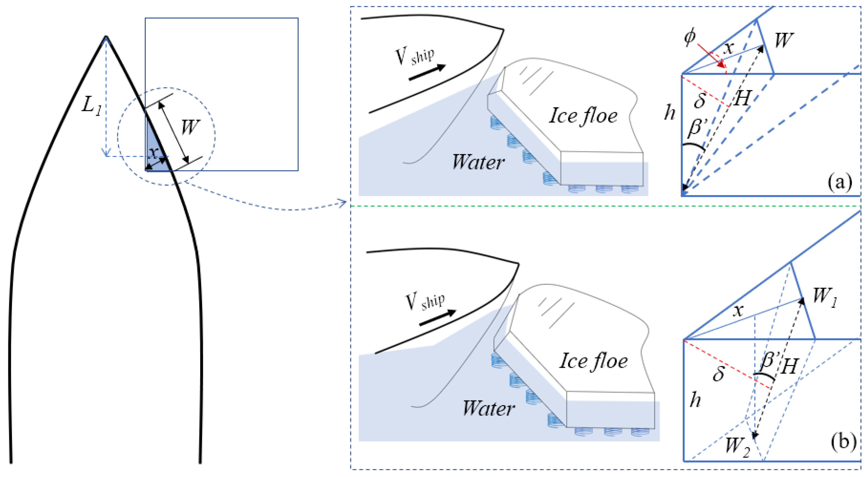
2.2. Maximum Depth of the Hull’s Penetration into an Ice Floe

The ship and ice floe can be regarded as a closed system during the collision situation. This study analyzed the consistency between the velocity at the ship–ice contact point and the translational velocity of the floating ice. Specifically, if the normal velocity component at the ship–ice contact point matches the corresponding velocity component of the floating ice, this indicates that the two are synchronized in speed along the normal direction, thereby preventing further pressing or wedging of the hull into the ice.

An ice floe under the influence of the current will produce accelerated motion, resulting in inertial forces, in which the added mass is proportional to the volume of water in which the ice floe is immersed. The added mass of crushed ice is as follows:

$$M_a=C_m{\rho }_w{V}_{sub}{a}_{\mathrm{ice}}$$

(4)

where C_m is the additional mass coefficient, Lamb [24] and Zong [25] defined C_m = 1 for circle ice and C_m = 1.189 for square ice; ρ_w is the water density; V_sub is the submerged volume of ice; and a_ice is the acceleration of ice.

Therefore, the total ice mass should be solved based on Equation (5):

$$M_{ice}=m_{ice}+M_a$$

(5)

Because the hull is set to a constant speed, the collision process between the ship and ice does not allow for the law of conservation of energy. Consequently, this study uses the impulse theorem to transform the force exerted by the hull into the translational velocity of the ice mass. Throughout the duration defined as Δt, during which the ship penetrates the deepest depth of ice, we consider the following:

$${\displaystyle \underset{0}{\overset{\Delta t}{\int }}{F}_{xf}tdt}=M_{ice}{V}_{ice}$$

(6)

When the ice velocity (V_ice) is equal to V_shipsin(α), the ship penetrates to its maximum depth (δ). Consequently, we can derive the ship–ice interaction time as follows:

$${\displaystyle \frac{1}{2}}{V}_{ship}\sin \alpha \Delta t^2=\delta \to \Delta t=\sqrt{{\displaystyle \frac{2\delta }{V_{ship}\sin \alpha }}}$$

(7)

After substituting the above formula, we obtain

$${\displaystyle \frac{\delta F_{\delta }\cos \left({\beta }^{\prime }\right)}{V_{ship}\sin \alpha }}{=\mathrm{M}}_{ice}{V}_{ship}$$

(8)

The maximum penetration depth, denoted as δ, can be determined by substituting the extrusion pressure F(δ) into the aforementioned formula. However, if the ice has an initial speed, it will suffer from water resistance. To accurately describe the behavior of the ice floe, it is essential to calculate both the water resistance and the torque generated by the ice. The equations for water resistance and the corresponding moment of resistance are as follows:

$$\begin{array}{l}{F}_{water}={\displaystyle \frac{1}{2}}{C}_d{\rho }_w{A}_{obl}{V}_{ice}^2\\ T_{water}={\displaystyle \frac{1}{2}}{C}_a{\rho }_w{l}_{ice}^3{A}_{ice}{w}_{ice}^2\end{array}$$

(9)

where the coefficients of action and resistance are C_d and C_a, respectively. According to Biye Yang’s research, C_d is 1 and C_a is 0.05 in this study. ρ_w is the density of water; A_ice is the area of the ice body submerged in water; and A_obl is the projected area of A_ice with velocity V_ice along the ice cube, as shown in Figure 6. l_ice is the average length of the ice floe, and the averages of the length, width, and thickness of the ice are used.

Considering water resistance, the impulse theorem becomes

$${\displaystyle \underset{0}{\overset{\Delta t}{\int }}\left(F_{xf}-F_{water}\right)tdt}=M_{ice}{V}_{ship}$$

(10)

In the iterative numerical calculations, the maximum penetration depth and duration of the ship–ice interaction, denoted as Δt, can be determined by substituting the extrusion pressure F_δ into the aforementioned equation. Additionally, during collision, the ice also experiences rotation as a result of the combined forces from the ship–ice friction and F_xy. The torque generated by this rotational motion can be expressed as the product of the resultant force and the vertical distance (r) from the center of rotation of the floating ice. According to the angular momentum theorem, the angular acceleration of the floating ice can be derived as follows:

$$T_{sum}=F_{\delta }\cos \left({\beta }^{\prime }\right)r-T_{water}=I_{ice}{\alpha }_{ice}$$

(11)

Once the angular acceleration is obtained, the rotational angular velocity of the floating ice can be calculated based on the previously determined ship–ice collision time:

$$w_{ice}=a_{ice}\Delta t$$

(12)

2.3. Unbreakable Ice Floes

According to Hetényi’s [26] definition of finite beams, Wenjun Lu [19] and Kim [20] defined the limit size beyond which ice deflection under a vertical force can be disregarded. Assuming a Poisson ratio of 0.3, they calculated that the maximum size for an “unbreakable ice floe” is approximately 1.08 times the characteristic length, essentially equating it to the characteristic length itself. The definition of a “characteristic length” is as follows:

$$l=\sqrt[4]{{\displaystyle \frac{D}{k}}}=\sqrt[4]{{\displaystyle \frac{E{h}^3}{12\left(1-v^2\right){\rho }_{w}g}}}$$

(13)

where D is the flexural rigidity, k is the foundation modulus, E is the modulus of elasticity, h is the ice thickness, v is the Poisson ratio, ρ_w is the water density, and g is the gravitational acceleration.

Based on field navigation experience and observations from ice tank tests, the concept of an “unbreakable ice floe” should be expanded to include large ice floes that cannot be broken. Consequently, this study adopts a broad definition of “unbreakable floating ice”, referring to any ice floe that does not fracture upon impact. The determination of whether large floating ice will be damaged is based on specific criteria detailed in the following sections.

2.4. Breakable Ice Floes

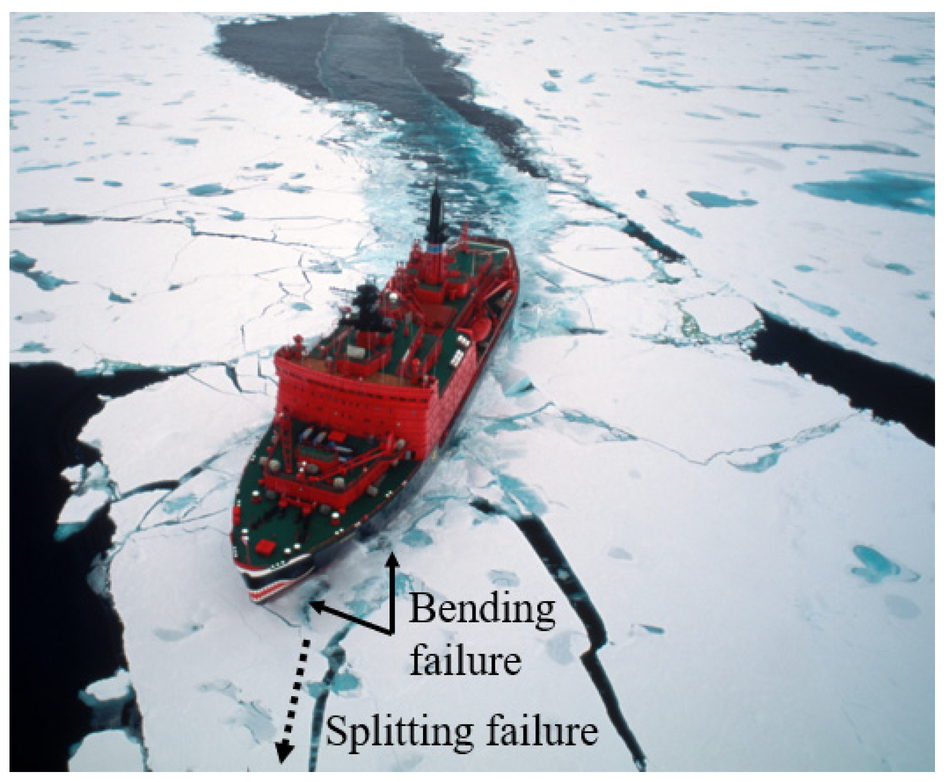
2.4.1. Bending Failure

Numerous studies have focused on bending failure. Researchers such as Kerr [27], Nevel [28], Paavilainen [29], and Lubbad [18] have identified flexural strength as a crucial parameter for determining ice failure. If the internal stress exceeds the flexural strength, bending failure will occur. In this study, bending failure is assessed by comparing the maximum principal stress with the flexural strength. The criteria for this comparison are as follows:

$${\sigma }_1>{\sigma }_f$$

(14)

where σ₁ is the maximum principal stress within the ice floe and σ_f is the flexural strength of the ice. For the solution of the maximum principal stress, please refer to Section 3.2.

2.4.2. Splitting Failure

Field ship navigation observations and experimental data demonstrate that splitting failure may occur when an ice floe is impacted by a ship’s stem. Such failures can be analyzed based on fracture mechanics. Classical fracture mechanics include Linear Elastic Fracture Mechanics (LEFMs) and Nonlinear Fracture Mechanics (NLFMs). LEFMs utilize linear elasticity theory to study crack propagation in materials, while NLFMs incorporate both elasticity and plasticity theories, making them particularly suitable for scenarios where a large plastic zone develops near the crack tip. There is still a debate about whether LEFMs or NLFMs are more suitable for analyzing the splitting failure of ice floes. Bhat [30,31] showed that large-scale ice floes behave as brittle materials. Based on this perspective, Bhat used the Finite Element Method (FEM) based on LEFMs to analyze the splitting failure of square ice floes. Similarly, experiments by Dempsey [32] on square ice floes concluded that crack propagation in ice can be directly analyzed using LEFMs. Lu et al. [15] conducted FEM studies on ice splitting using methodologies with the following combinations: “LEFM + weight function” and “Cohesive Zone Model (CZM) + weight function”. They obtained similar conclusions to those of Bhat and Dempsey.

In this study, an ice floe is considered a linear elastic material. The process of crack propagation in classical fracture mechanics involves three principal stages: crack initiation, crack propagation, and crack instability propagation. This study discusses each of these three stages. In ice mechanics, crack initiation refers to the presence of defects in the microstructure of ice materials, causing stress concentration and local cracking at the tip of the defect. This stress is defined as theoretical cracking stress. Researchers such as Wenjun Lu [15], Lubbad [18], and Yihe Wang [33] utilized the maximum bending stress at the point of action to determine crack initiation:

$${\sigma }_{yy}(0,0)={\sigma }_f$$

(15)

where σ_f is the flexural strength of ice, and σ_yy is the bending stress at the force position.

Crack initiation occurs when the stress reaches the theoretical cracking stress. It is well-established that cracks generally originate from structural defects. This phenomenon is especially common in bow–ice collision scenarios, where these defects mainly result from compressive failures caused by the ship’s stem becoming embedded in the ice. Therefore, it is logical to consider the area impacted by this compressive failure as the initial crack. This assumption is supported by researchers such as Wenjun Lu [15] and Yihe Wang [33].

LEFMs demonstrate that materials possess inherent resistance to crack propagation; thus, cracks will only propagate under sufficiently high tensile stresses. The critical parameter is the fracture toughness, as defined in Equation (21). A crack will continue to propagate only if the stress intensity factor at its tip exceeds the fracture toughness threshold. In this study, the stress intensity factor at the crack tip was calculated using the Wu–Carlsson weight function method [34,35].

$$\begin{gathered} K_I=f\sigma \sqrt{\pi A} \\ \sigma ={\displaystyle \frac{F_{\sigma }}{S}}\cos {\beta }^{\prime }\cos \alpha \end{gathered}$$

(16)

where f is the dimensionless stress intensity factor calculated using Equation (15) (unitless); σ is the tensile stress (i.e., the transverse stress) (Pa); and A is the crack length (m), which can be identified in the simulation process. Wu and Xu [35] developed the finite sums of the dimensionless stress intensity factor as follows:

$$f={\displaystyle \frac{2^{0.5}\alpha }{\pi }}{\displaystyle \sum _{i=1}^5{\beta }_i\left(\alpha \right)\frac{1}{2i-1}}$$

(17)

where α is the crack ratio, which is the ratio of the crack length A to the longitudinal penetration length L.

$$\alpha ={\displaystyle \frac{A}{L}}$$

(18)

$$\begin{array}{l}{\beta }_1\left(\alpha \right)=2\\ {\beta }_2\left(\alpha \right)={\displaystyle \frac{1}{{\left(1-\alpha \right)}^{3/2}}}\left[\left(828.1465\alpha -930.6541\right)\sqrt{1-\alpha }+931.6343-1294.0176\alpha +333.3853{\alpha }^2-26.1606{\alpha }^3+65.9137{\alpha }^4\right]\\ {\beta }_3\left(\alpha \right)={\displaystyle \frac{1}{{\left(1-\alpha \right)}^{3/2}}}\left[\left(202.3555\alpha -294.3217\right)\sqrt{1-\alpha }+295.4271-350.9952\alpha +63.7728{\alpha }^2+21.1496{\alpha }^3\right]\\ {\beta }_4\left(\alpha \right)={\displaystyle \frac{1}{{\left(1-\alpha \right)}^{3/2}}}\left[\left(-155.2612\alpha +253.9361\right)\sqrt{1-\alpha }-254.2507+282.0580\alpha -42.0427{\alpha }^2-11.2951{\alpha }^3\right]\\ {\beta }_5\left(\alpha \right)={\displaystyle \frac{1}{{\left(1-\alpha \right)}^{3/2}}}\left[\left(35.2302\alpha -66.5987\right)\sqrt{1-\alpha }+66.4954-68.0570\alpha +8.3261{\alpha }^2+1.3405{\alpha }^3\right]\end{array}$$

(19)

Once the stress intensity factor at the crack tip exceeds the fracture toughness, the crack will propagate forward. The material’s ability to resist further crack propagation can be quantified by the surface energy, which is denoted by γ [36]. The surface energy represents the energy required to generate a new crack surface per unit length. In fracture mechanics, crack propagation is assumed to be a quasi-static event. This process is described by the energy release rate (G), which refers to the energy released per unit thickness. This index provides a quantitative basis for assessing the dynamics of crack propagation in terms of energy consumption and distribution.

$$G\left(B\Delta a\right)=\gamma \left(2B\Delta a\right)$$

(20)

The Griffith fracture criterion can be expressed as follows:

$$G=2\gamma$$

(21)

Irwin posited that the work exerted by forces (W) on a system is converted into different forms of energy: stored strain energy (U), kinetic energy (T), and irrecoverable dissipated energy (D). The energy balance is as follows:

$${\displaystyle \frac{dW}{dt}}={\displaystyle \frac{dU}{dt}}+{\displaystyle \frac{dT}{dt}}+{\displaystyle \frac{dD}{dt}}$$

(22)

Under the quasi-static condition, where the crack remains either stationary or propagates at a constant velocity, it is assumed that the kinetic energy remains unaltered. Hence, we have

$${\displaystyle \frac{dT}{dt}}=0$$

(23)

Assuming that all the irrecoverable dissipated energy is utilized for the creation of a new crack surface area, the energy balance equation can be reformulated as follows:

$${\displaystyle \frac{dD}{dt}}={\displaystyle \frac{dD}{dA}}{\displaystyle \frac{dA}{dt}}={\gamma }_p{\displaystyle \frac{dA}{dt}}$$

(24)

where ${\gamma }_p$ denotes the energy required to form a unit area of crack surface. When there is negligible or minimal plastic deformation at the crack tip, ${\gamma }_p$ equals the surface energy. However, if significant plastic deformation occurs, additional energy is needed to create a new crack surface, i.e., ${\gamma }_p>\gamma$. In this study, this equation can, thus, be further expressed as

$${\displaystyle \frac{d\left(W-U\right)}{dA}}={\gamma }_p$$

(25)

Considering the previously mentioned single-edge crack with a length denoted as “A”, the crack creates two symmetrical surfaces. Consequently, the total area of the crack can be expressed as 2hA. Therefore,

$${\displaystyle \frac{1}{2h}}{\displaystyle \frac{d\left(W-U\right)}{dA}}={\gamma }_p$$

(26)

Based on Griffith theory, we can further clarify the relationship between the energy release rate and the previously mentioned equation:

$${\displaystyle \frac{1}{h}}{\displaystyle \frac{d\left(W-U\right)}{dA}}=G$$

(27)

Based on the linear elastic materials of ice, the strain energy equals half the work performed by the external forces. Consequently, we obtain the following relationship:

$${\displaystyle \frac{1}{h}}{\displaystyle \frac{d\left(W-U\right)}{dA}}={\displaystyle \frac{1}{h}}{\displaystyle \frac{dU}{dA}}=G$$

(28)

As for the driving forces of crack propagation, this study assumes that F_x is the principal driving force for the translational motion of an ice floe, while F_z and F_y are the key forces driving crack propagation. Under this assumption, the displacements driven by Fz and Fy are represented by w(A) and u(A), respectively. Consequently, the above equation is changed as follows:

$$G={\displaystyle \frac{1}{h}}{\displaystyle \frac{dU}{dA}}={\displaystyle \frac{1}{2h}}{\displaystyle \frac{Fzdw\left(A\right)+Fydu\left(A\right)}{dA}}$$

(29)

Here, the non-dimensional function is introduced as follows:

$$W\left(A\right)={\displaystyle \frac{w\left(A\right)D}{F_z{L}^2}},C\left(A\right)={\displaystyle \frac{u\left(A\right)E}{\left(F_y/t\right)}}$$

(30)

The equation also can be further refined as follows:

$$G={\displaystyle \frac{{12}^{3/4}}{2k^{1/4}}}n{\displaystyle \frac{F_z^2}{t^{13/4}}}{\displaystyle \frac{dW\left(\alpha \right)}{d\alpha }}{\left[{\displaystyle \frac{\left(1-{\nu }^2\right)}{E}}\right]}^{3/4}+{\displaystyle \frac{n{F}_y^2}{{\left(12\left(1-{\nu }^2\right)k\right)}^{1/4}{E}^{3/4}{t}^{5/4}}}{\displaystyle \frac{dC\left(\alpha \right)}{d\alpha }}$$

(31)

According to the stem shape parameters, we have

$$F_z=F_y\tan \left({\beta }^{\prime }\right)\cos \left(\alpha \right)$$

(32)

Substituting Equation (34) into Equation (33):

$$G=F_y^{2}n\left[{\displaystyle \frac{{12}^{3/4}}{2k^{1/4}}}{\displaystyle \frac{{\left(\tan \left({\beta }^{\prime }\right)\cos \left(\alpha \right)\right)}^2}{t^{13/4}}}{\displaystyle \frac{dW\left(\alpha \right)}{d\alpha }}{\left[{\displaystyle \frac{\left(1-{\nu }^2\right)}{E}}\right]}^{3/4}+{\displaystyle \frac{1}{{\left(12\left(1-{\nu }^2\right)k\right)}^{1/4}{E}^{3/4}{t}^{5/4}}}{\displaystyle \frac{dC\left(\alpha \right)}{d\alpha }}\right]$$

(33)

The value of ${\displaystyle \frac{dW\left(\alpha \right)}{d\alpha }}$ and ${\displaystyle \frac{dC\left(\alpha \right)}{d\alpha }}$ can be calculated based on the research of Wenjun Lu [15].

Once a crack reaches a critical length, it transitions from stable to unstable propagation. The transition threshold is defined by the ratio of the crack propagation length to the ice floe length, which correlates with the width-to-length ratio of the ice floe. Specifically, research conducted by Bhat [31] and Lu [15] indicates that unstable failure of a square ice floe occurs when the crack propagates to 14.5% of the ice floe length. Therefore, this study adopted the 14.5% criterion as a key index for evaluating the splitting failure of ice floes.

3. Numerical Simulation Method for Ship Navigation in Ice-Covered Waters

3.1. General Assumptions

This study conducted a numerical simulation investigation of ship–ice collisions, leveraging insights from sea ice theory and ice tank model tests. Due to the complexities of field ship–ice interaction scenarios and the focus on two-dimensional simulations, the following simplified assumptions were made:

(1)

Kirchhoff Plate Model: The ice floe was modeled as a Kirchhoff plate, which is supported by a Winkler elastic foundation of seawater. According to Ventsel [37], the ratio of the characteristic length of the plate to its thickness should be greater than 10. Based on research by Lu et al. [15] and Gold [38] on sea ice, the characteristic length of sea ice is approximated to be 13.5 times the ice thickness. Consequently, the appropriate thickness limit for applying Kirchhoff plate theory is h < 3.32 m, which encompasses the range of most observed ice thicknesses.

(2)

Brittle Material Assumption: Sea ice was treated as a brittle material. The loading rate during the ship’s interaction with the ice is sufficiently high to inhibit creep behavior.

(3)

Material Homogeneity and Isotropy: This study focused on first-year sea ice, which is largely columnar in structure and demonstrates various anisotropic mechanical behaviors (Sanderson [16]) along with temperature gradients that occur along the ice thickness. However, because radial and circumferential fractures typically develop perpendicular to the columnar structure, it is reasonable to treat the ice as isotropic and overlook the impacts of temperature fluctuations.

(4)

Geometry of Ice Floes: According to Hamilton [39], downstream-managed ice floes often present a 1:1 aspect ratio. Although circular ice floes are more commonly found at the edges of ice-covered regions, for this theoretical exploratory study, the assumption of square ice floes was considered suitable. This approach is consistent with assumptions used in ice tank testing processes, as documented by Hoving [40].

(5)

Dynamic Fluid Base Effects: The dynamic effects of the fluid base on the ice floe were neglected, with a focus on the resistance characteristics.

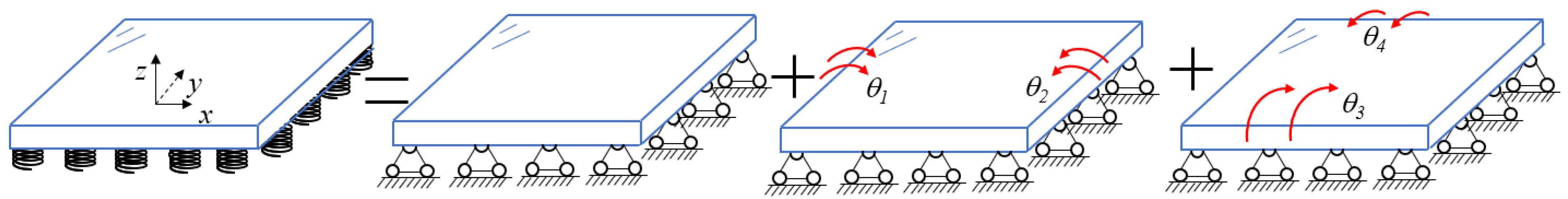
3.2. Deflection Equation and Analytical Solution

Floating ice on the sea surface can be modeled as a Winkler plate, with the seawater acting as an elastic foundation, as depicted in Figure 7. According to Kirchhoff’s theory, the formulation of a thin plate under a concentrated load is expressed as follows, and the symbol explanations are summarized in

Table 1. The definitions and methodology for solving each symbol.

Symbol	Meaning of Symbol	Unit
q(x,y)	Concentrated load	N
w(x,y)	Transverse deflection at point (x, y) of the plate in the z-direction under a lateral concentrated load	m
hice	Thickness of the ice floe	m
E	Young’s modulus of ice	Pa
v	Poisson’s ratio	-
$D={\displaystyle \frac{E{h}_{ice}^3}{12\left(1-v^2\right)}}$	Flexural rigidity of the plate with symbols explained below	Nm
${\nabla }^4\left(\right)={\displaystyle \frac{{\partial }^{4}w}{\partial x^4}}+2{\displaystyle \frac{{\partial }^{4}w}{\partial x\partial y}}+{\displaystyle \frac{{\partial }^{4}w}{\partial y^4}}$	Biharmonic operator	-
ρw	Fluid density	kg/m3
g	Gravitational acceleration	m/s2
k = ρw × g	Foundation modulus	Pa/m

.

$$D{\nabla }^4\left(w\right)+kw=q\left(x,y\right)$$

(34)

According to Li Rui [21], the deflections of an elastic foundation plate with free edges are calculated by dividing the problem into three types of boundary conditions, as illustrated in Figure 8. The flexural equilibrium equations corresponding to each boundary condition are solved individually. Once these separate solutions are obtained, they are superimposed to determine the overall deflection that satisfies the initial free boundary conditions, as expressed in Equation (40). For a detailed description of the method, readers are referred to Li Rui’s original work.

$$w\left(x,y\right)=w_1\left(x,y\right)+w_2\left(x,y\right)+w_3\left(x,y\right)$$

(35)

According to the generalized Hooke’s law,

$$\begin{array}{l}{\sigma }_x={\displaystyle \frac{E}{1-{\upsilon }^2}}\left({\epsilon }_x+\upsilon {\epsilon }_y\right)=-{\displaystyle \frac{Ez}{1-{\upsilon }^2}}\left({\displaystyle \frac{{\partial }^{2}w}{\partial x^2}}+\upsilon {\displaystyle \frac{{\partial }^{2}w}{\partial y^2}}\right)\\ {\sigma }_y={\displaystyle \frac{E}{1-{\upsilon }^2}}\left({\epsilon }_y+\upsilon {\epsilon }_x\right)=-{\displaystyle \frac{Ez}{1-{\upsilon }^2}}\left({\displaystyle \frac{{\partial }^{2}w}{\partial y^2}}+\upsilon {\displaystyle \frac{{\partial }^{2}w}{\partial x^2}}\right)\\ {\tau }_{xy}={\displaystyle \frac{E}{2\left(1+\upsilon \right)}}{\epsilon }_{xy}=-{\displaystyle \frac{Ez}{\left(1+\upsilon \right)}}{\displaystyle \frac{{\partial }^{2}w}{\partial x\partial y}}\end{array}$$

(36)

The maximum principal stress can be calculated using the following formula:

$${\sigma }_{1,2}={\displaystyle \frac{{\sigma }_x+{\sigma }_y}{2}}\pm \sqrt{{\left({\displaystyle \frac{{\sigma }_x-{\sigma }_y}{2}}\right)}^2+{\tau }_{xy}^2}$$

(37)

3.3. Analysis of the Ship–Ice Collision Process

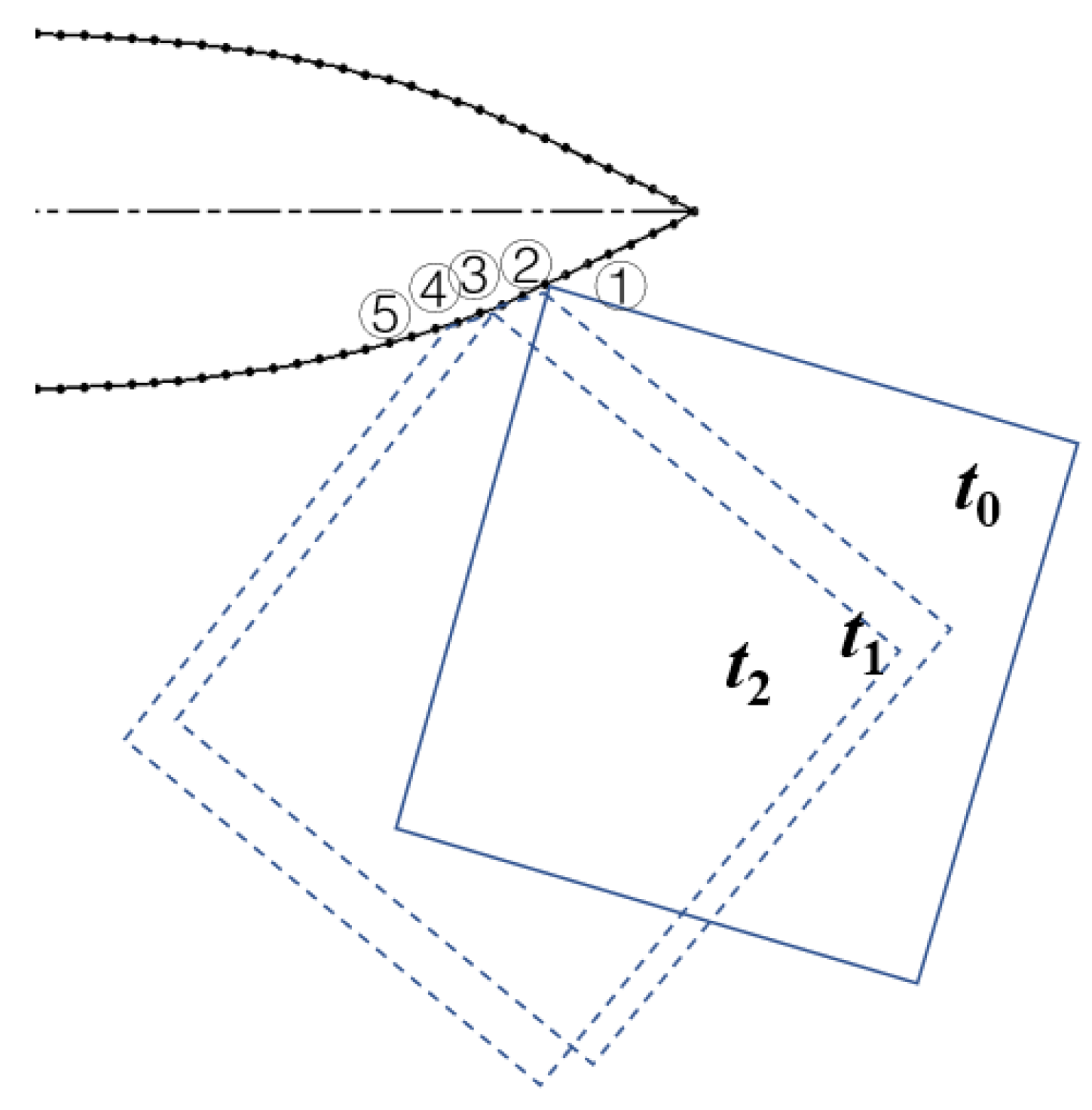
3.3.1. Movement of Ice Along the Ship Hull

In this study, to accurately simulate the interaction forces between the ice floe and the hull, the ship’s contour is meticulously subdivided into uniformly spaced segments, as shown in Figure 9. The ship’s surface is divided into a series of equally spaced stations, and ice loads are applied to these specific stations, as detailed below:

(1)

At t₀, the ice load is applied to station ①, representing the initial point of contact.

(2)

At t₁, the ice load is evenly distributed at stations ② and ③, simulating the spreading of forces as the ship continues to move through the ice.

(3)

At t₂, the load is further spread to stations ④ and ⑤.

3.3.2. Analysis of Ice Movement

In this study, the translational and angular velocities of ice floes impacting ships are calculated using the principles of momentum and angular momentum conservation. The translational displacement and rotation angle of the ice floe are computed iteratively at each time step. Regarding ice floe interactions, this study assumes momentum conservation and considers the initial collision stage to be elastic. The masses of the two colliding ice floes are denoted as m₁ and m₂, with initial velocities u₁ and u₂, respectively. After the collision, the velocities change to v₁ and v₂. The conservation of momentum is expressed as follows:

$$m_1{\overrightarrow{u}}_1^i+m_2{\overrightarrow{u}}_2^i=m_1{\overrightarrow{v}}_1^i+m_2{\overrightarrow{v}}_2^i$$

(38)

where i is the x or y direction.

According to the conservation of energy, we have

$${\displaystyle \frac{1}{2}}{m}_1{\overrightarrow{u}}_1^i{}^2+{\displaystyle \frac{1}{2}}{m}_2{\overrightarrow{u}}_2^i{}^2={\displaystyle \frac{1}{2}}{m}_1{\overrightarrow{v}}_1^i{}^2+{\displaystyle \frac{1}{2}}{m}_2{{\overrightarrow{v}}_2^i}^2$$

(39)

By solving the simultaneous equations above, the velocities of the two ice floes after the collision are

$$\begin{array}{l}{v}_1^i={\displaystyle \frac{m_1-m_2}{m_1+m_2}}{u}_1^i+{\displaystyle \frac{2m_2}{m_1+m_2}}{u}_2^i\\ v_2^i={\displaystyle \frac{2m_1}{m_1+m_2}}{u}_1^i+{\displaystyle \frac{m_2-m_1}{m_1+m_2}}{u}_2^i\end{array}$$

(40)

When the ice floe moves away from the ship, it is only subjected to water resistance F_water and water torque T_water. The translational acceleration and rotational acceleration can be calculated based on Equation (46):

$$\begin{array}{l}{F}_{water}={\displaystyle \frac{1}{2}}{C}_d{\rho }_w{A}_{obl}{V}_{ice}^2=M_{ice}a\\ T_{water}={\displaystyle \frac{1}{2}}{C}_a{\rho }_w{l}_{ice}^3{A}_{ice}{w}_{ice}^2=I_{ice}\alpha \end{array}$$

(41)

The translational and rotational velocity of the ice in a single time step are calculated as follows:

$$\begin{array}{l}{V}_{ice}^{t+dt}=V_{ice}-adt\\ w_{ice}^{t+dt}=w_{ice}-\alpha dt\end{array}$$

(42)

The changes in ice displacement and the rotation angle are calculated as follows:

$$\begin{array}{l}\Delta D_{ice}^{t+dt}=\left(V_{ice}-adt\right)dt\\ \Delta A{n}_{ice}^{t+dt}=\left(w_{ice}-\alpha dt\right)dt\end{array}$$

(43)

3.4. Collision Detection Algorithm

In numerical simulations, two primary types of collisions must be considered: ship-to-ice and ice-to-ice interactions. Detecting ice-to-ice collisions on an individual basis significantly decreases the computational efficiency of the numerical algorithm, necessitating the development of a fast collision detection method. This study employs the Sweep and Prune (SAP) algorithm in conjunction with the Gilbert–Johnson–Keerthi (GJK) algorithm to enhance the efficiency of collision detection in such simulations.

3.4.1. Sweep and Prune Algorithm (SAP)

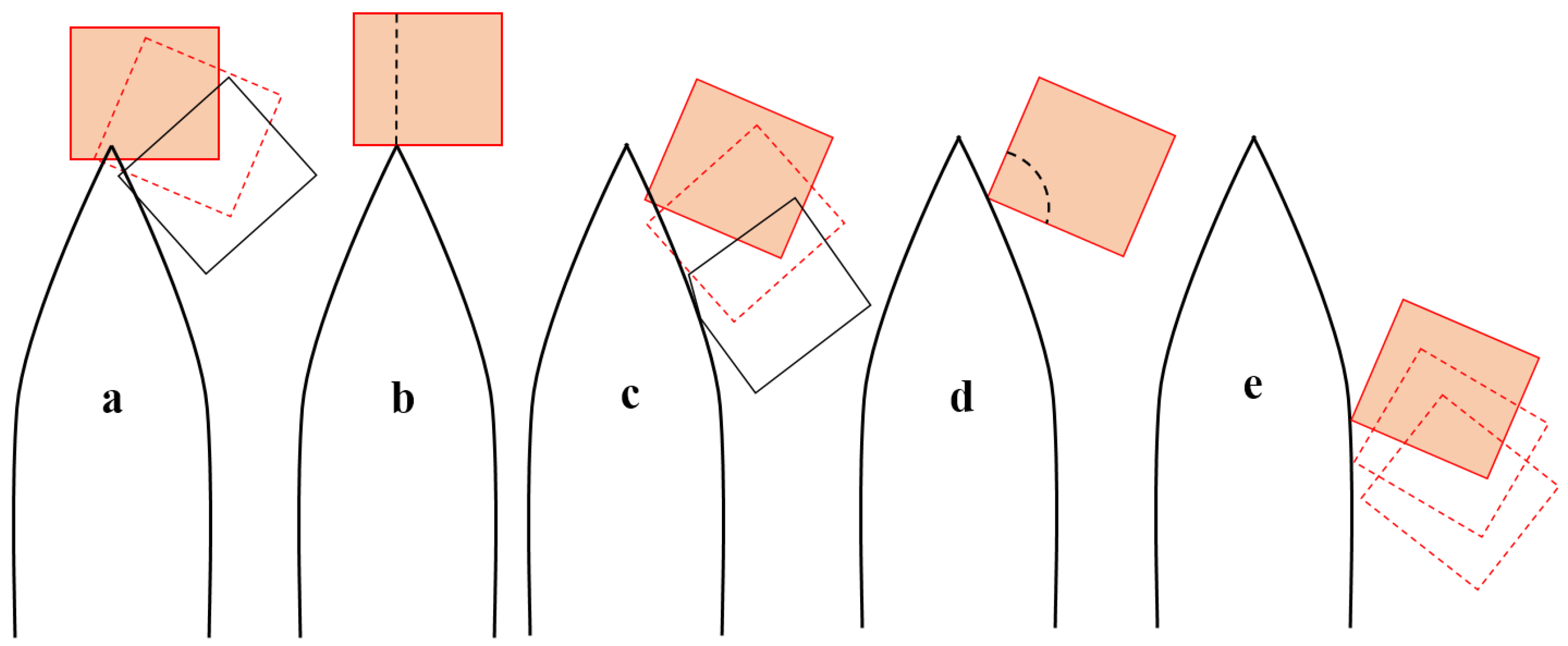
The Sweep and Prune (SAP) algorithm is a computational geometry method used to efficiently detect potential collisions between objects in two-dimensional space, as depicted in Figure 10, step by step.

The Sweep and Prune (SAP) algorithm, a computational geometry method, is employed to efficiently detect potential collisions between objects in two-dimensional space. The algorithm proceeds through the following steps:

(1)

Recording Corner Coordinates: The coordinates of the corners of all Axis-Aligned Bounding Boxes (AABBs) are recorded in separate lists for the X- and Y-axes. As shown in Figure 10a, the minimum (1L) and maximum (1U) values of the x-axis and of the minimum (1L) and maximum (1U) values of the y-axis of object 1 have been added in Figure 10b.

(2)

Sorting the Lists: These lists of Figure 10b are sorted in ascending order based on the coordinates. This sorting process is crucial, as it allows the algorithm to efficiently prune non-colliding pairs in the subsequent steps.

(3)

Intersection of Bounding Boxes: Overlapping intervals are checked in the sorted lists, as shown in Figure 10b. The intersection of bounding boxes is confirmed when their intervals overlap in both the X and Y lists. For example, the intersection of bounding boxes corresponding to objects 2 and 3 indicates that they are potential collision pairs.

The SAP algorithm is particularly advantageous in physics simulations, where the swift detection of potential collisions is essential for real-time performance. By effectively reducing computational resources, the SAP algorithm enables more complex simulations with a greater number of objects without significantly sacrificing performance.

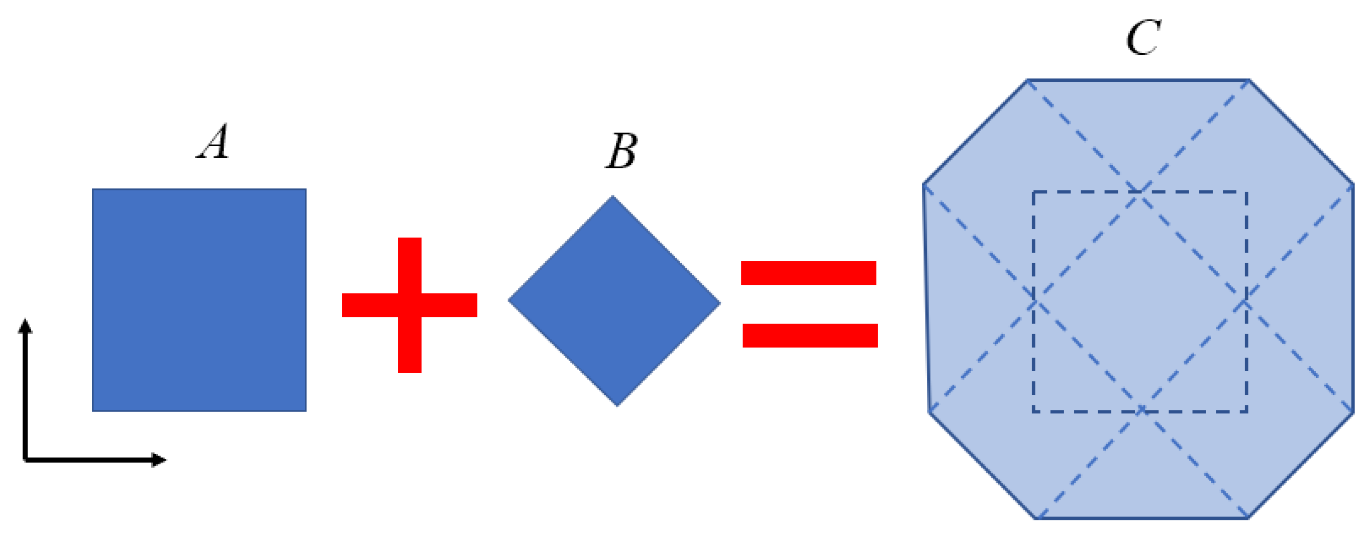
3.4.2. Gilbert–Johnson–Keerthi (GJK) Algorithm

The Gilbert–Johnson–Keerthi (GJK) algorithm is a robust and efficient method employed in computational geometry to determine whether two convex shapes intersect. The algorithm’s effectiveness lies in its utilization of the Minkowski difference and the Minkowski sum, which are fundamental to its operation.

$$A+B=\{a+b:a\in A,b\in B\}$$

(44)

Figure 11 illustrates the concept of the Minkowski sum (denoted as A⊕B), which can be interpreted as the outcome of translating point set B along the boundary of point set A. Analogously, the Minkowski difference (A − B) can be obtained by employing the Minkowski sum operation.

$$A-B=A+(-B)=\{a-b:a\in A,b\in B\}$$

(45)

If point sets A and B have overlapping points, the Minkowski difference will inevitably include the origin point. This concept is fundamental to the Gilbert–Johnson–Keerthi (GJK) algorithm when used to detect contact.

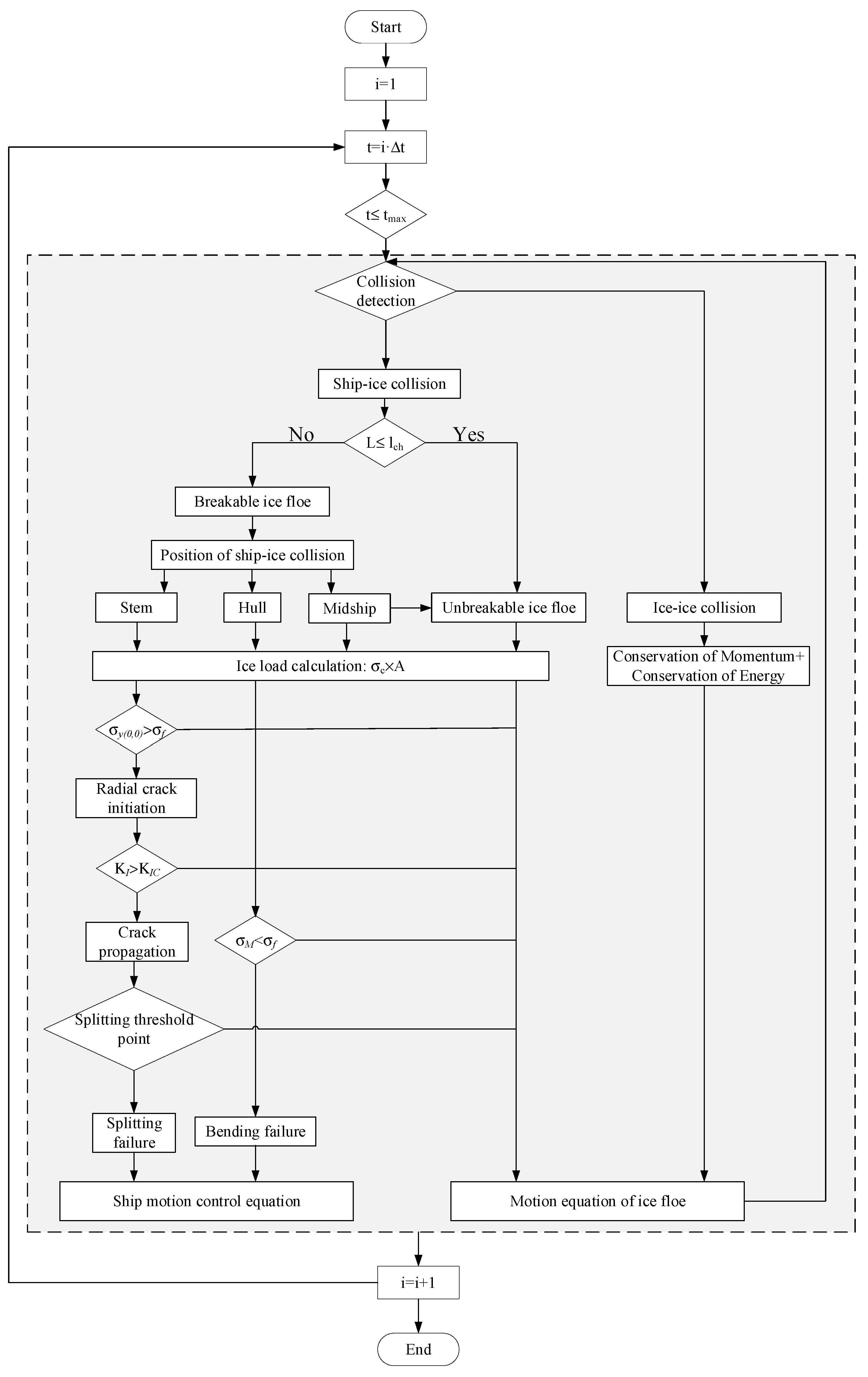
3.5. Process of Numerical Simulation

The section above thoroughly explores techniques for determining ice failure modes, estimating ice loads, and evaluating ship dynamics. Herein, a comprehensive numerical algorithm that is tailored for vessels navigating through ice-covered waters is presented. Figure 12 illustrates a detailed flowchart of the calculation. The program had been developed based on Figure 12. The theory of the ice load calculation method, ice failure identification method, SAP algorithm, and GJK method are used in this program. Empirical data such as extreme values of ice splitting and the friction coefficient are applied.

4. Verification of the Accuracy of the Numerical Simulation Method

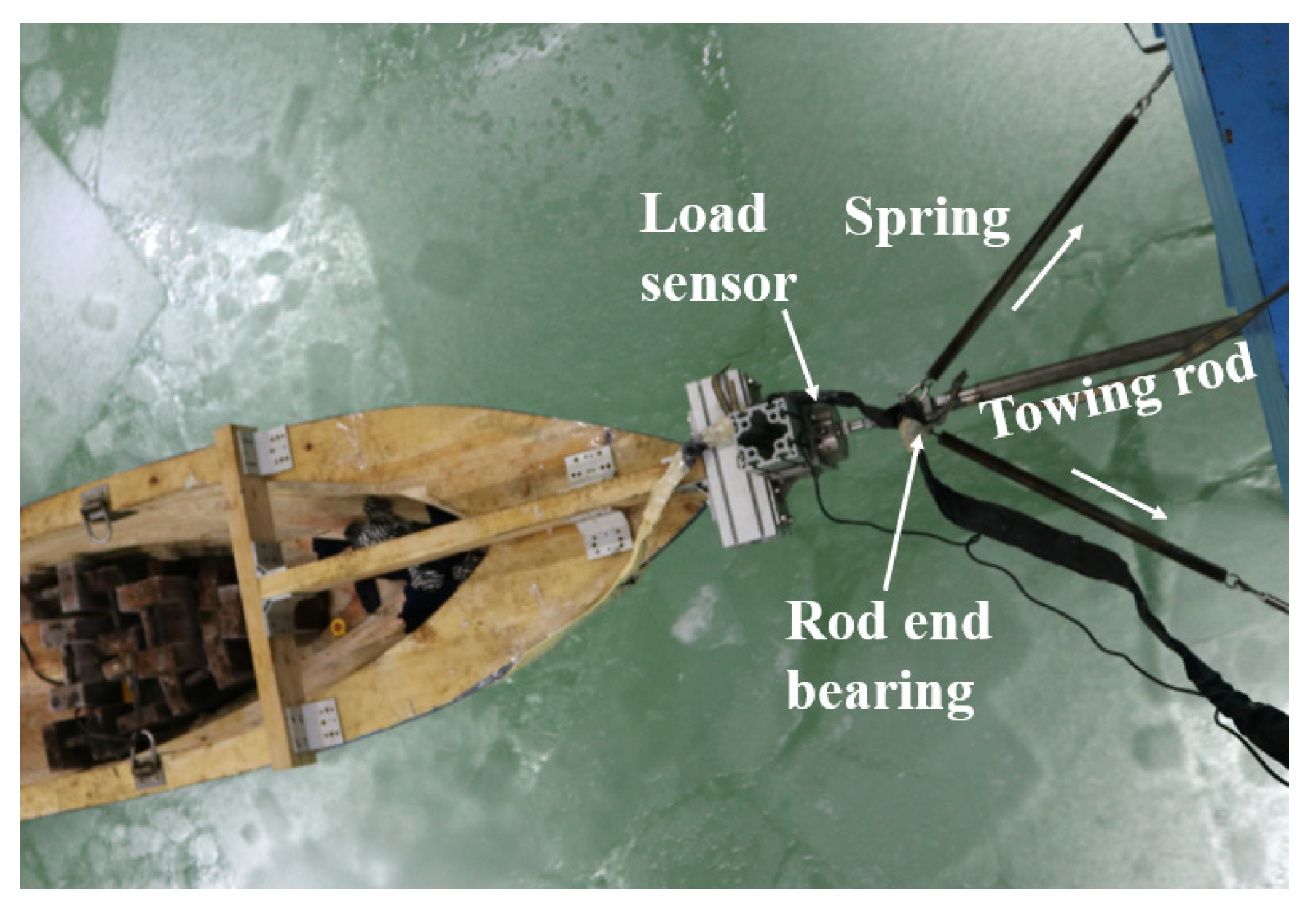
4.1. Test Facility

To verify the accuracy of the numerical method described above, we compared the results of ice tank tests with those obtained from numerical simulations. Model tests were conducted at the Ice Engineering Laboratory of Tianjin University. The low-temperature space of the laboratory is 320.0 m², and the ice tank is 40 × 6 × 2 m. The maximum driving force of the carriage is 5 t, and the speed can be adjusted without steps in the range of 1 mm/s–1.0 m/s. The main parameters of the towing test system are depicted in Figure 13.

This test setup aimed to replicate the physical conditions that ships encounter in ice-covered waters, providing a robust basis for testing and validating the numerical simulations developed in this study. The data collected from these tests are crucial for refining the simulation algorithms and ensuring that they accurately reflect the complexities of ship–ice interactions. Moreover, the friction between the model ice pieces and the painted model hull was also measured. The average kinetic friction coefficient of ships was found to be approximately 0.06 at a sliding velocity of 0.5 m/s with an air temperature of −5 °C.

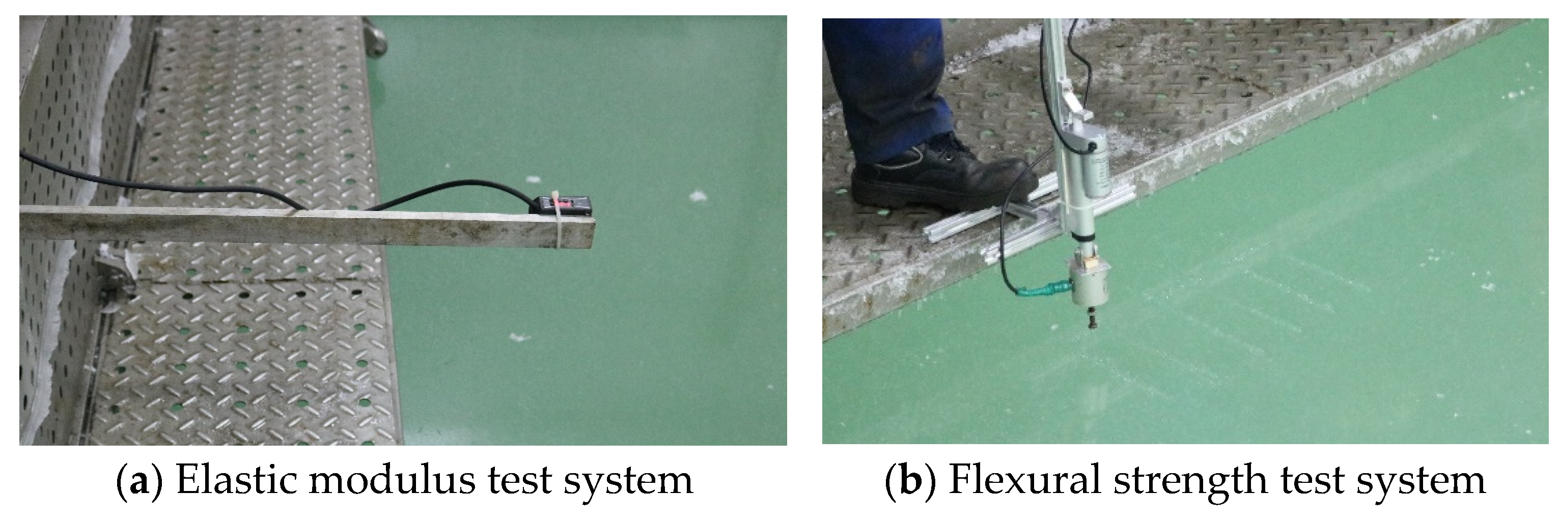
4.2. Measurement System for the Mechanical Properties of the Model Ice

The elastic modulus, flexural strength, and compressive strength of the model ice were measured based on specifically designed systems, as depicted in Figure 14. The data obtained from these measurements are crucial, as they provide essential inputs for numerical simulations.

4.2.1. Elastic Modulus Test

The elastic modulus of the model ice was measured using the infinite plate bending method. An elastic modulus testing system was developed for this purpose, as shown in Figure 14a. The system included a laser rangefinder with a 100 mm range and a measurement accuracy of 0.02 mm, an LWNA7108C current signal collector, standard weights, and a PVC sheet with a central hole. The use of the laser rangefinder allowed for precise non-contact measurement of the vertical deflection of the ice surface. The elastic modulus (E) is calculated using the following formula:

$$E={\displaystyle \frac{3}{16}}{\displaystyle \frac{1-{\upsilon }^2}{k{h}^3}}{\left({\displaystyle \frac{mg}{\xi }}\right)}^2$$

(46)

where m is the mass of the weight, g is the gravitational acceleration, k is the foundation modulus (k = g × ρ_w), h is the ice thickness, ξ is the displacement of the loading center point, and v is Poisson’s ratio.

4.2.2. Flexural Strength Test

The flexural strength of the model ice was measured using an in situ cantilever beam test method. The length (L) of the cantilever beam should be five to seven times the thickness of the ice, and the width (B) should be two to three times the thickness. A servo loader was utilized to apply a downward load at a fixed speed to the free end of the beam until the maximum bending force was reached, as shown in Figure 14b. The maximum linear stroke of the servo drive was 200 mm, with position control accuracy of 0.4 mm and a working speed range of 0.1 to 20 mm/s, with speed control accuracy of 0.02 mm. A force sensor, with a range of 200 N and accuracy of 0.1 N, was connected between the servo driver and the indenter to measure the loading force. The output from the force sensor was fed into a dynamic resistance strain gauge, which operated on 220 V AC and captured data at 100 Hz. The flexural strength was calculated using Equation (52):

$${\sigma }_f={\displaystyle \frac{6FL}{B{h}^2}}$$

(47)

where F is the maximum force at bending fracture, L is the distance from the loading point to the fracture position (length of the cantilever beam), B is the width of the cantilever beam, and h is the ice thickness.

4.2.3. Compressive Strength Test

This study measured the compressive strength of the model ice using the uniaxial compression test method. The ice mechanics testing device is depicted in Figure 14c,d. The testing system was designed to measure forces ranging from 100 N to 50 kN with a precision of ±0.2%. It featured an effective stroke of 800 mm and a displacement resolution of 0.02 μm. Additionally, the system’s speed control ranged from 0.001 to 500 mm/min, maintaining a speed accuracy of ±0.2%. The uniaxial compressive strength of the ice specimen was calculated using the following formula:

$${\sigma }_c={\displaystyle \frac{F}{A}}$$

(48)

where F is the maximum force when the ice is damaged, i.e., the maximum value in the loading time history curve; and A is the cross-sectional area of the ice.

4.3. Test Conditions

To verify the applicability of the numerical simulation method on different types of ships, this study conducted towing resistance tests using RV Xue Long. The main dimensional parameters of the ship are detailed in

Table 2. Main design parameters of the ship.

Parameter	Model Scale	Full Scale
Waterline length (m)	5.567	167.01
Waterline breadth (m)	0.753	22.59
Draught (m)	0.267	8.01
Displacement (ton)	0.779	21,025
Block coefficient	0.696
Wetted surface area (m2)	7.02	6319.3

, and the towing test conditions are outlined in

Table 3. Test conditions.

No.	Ice Thickness (m)	Concentration	Speed (m/s)
1	0.5	50%	188
2			282
3			376
4		70%	188
5			282
6			376

. The angle design parameters of this ship are shown in Figure 15. The scaling of parameters was based on the Froude and Cauchy similarity criteria, which are critical for ensuring the accuracy of model tests in fluid dynamics.

The Froude criterion, a fundamental similarity criterion used in fluid tests, assumes the dominance of gravity and inertial forces. The Froude number (Fr) is defined as follows:

$$Fr=U/\sqrt{gL}$$

(49)

where U is the velocity, g is the gravitational acceleration, and L is the geometric length.

Complementing the Froude number, the Cauchy criterion involves elastic and inertial forces:

$$Ca={\rho }_w{U}^2/E$$

(50)

where ρ_w is the water density, U is the velocity, and E is the elastic modulus.

It should be noted that the traditional Froude–Cauchy scaling approach was initially developed for the assessment of icebreaking resistance of ships and could be applicable for elastic reaction forces. Regarding the local ice failures during high-speed ship–ice impacts, where fractures and recrystallizations of ice are significant, the applicability of the Froude–Cauchy similarity may be questionable. Thus, these scaling laws were introduced in the present tests only as a basic approach to scaling down the prototype conditions. The scaling ratios for critical parameters such as ice strength, ice thickness, ice elastic modulus, and pressure under model conditions are consistent with the geometric scaling ratio, λ = 1:30. The scaling ratio for time and velocity is λ^1/2, and the scaling ratio for mass and force is λ³. The ice material parameters are summarized in

Table 4. Model ice properties.

Parameter	Value
Ice density	900 kg/m3
Ice modulus of elasticity	102.68 MPa
Poisson’s ratio	0.3
Water density	1025 kg/m3
Acceleration of gravity	9.81 m/s2
Flexural strength of ice	38.4 kPa
Compressive strength	107.52 kPa
Hull–ice friction coefficient	0.07

.

The elastic modulus, flexural strength, and compressive strength of model ice were measured based on specifically designed systems. The data obtained from these measurements are crucial, as they provide essential inputs for numerical simulations.

4.4. Iterative Time Step

In ship–ice collision scenarios, the selection of an appropriate iterative time step is crucial for striking a balance between computational demands and the accuracy and stability of the results. A judiciously chosen time step ensures that the simulation effectively captures the essential dynamic interactions. The time step for ship–ice collisions is intrinsically linked to the maximum penetration depth, which is a critical factor in the dynamics of these interactions. Considering these requirements, the formula for calculating the time step (dt) involves the speed of the ship (V_ship) and the maximum penetration depth (δ_M):

$$dt={\displaystyle \frac{{\delta }_M}{20V_{ship}\sin \left(\alpha \right)\cos \left({\beta }^{\prime }\right)}}$$

(51)

The angles of the ship’s hull, specifically, the waterline angle (α) and the normal frame angle (β’), along with the ice angle (ϕ), play a pivotal role in determining the appropriate time step for the simulation, as demonstrated in Equation (51). According to the theory proposed by Wenjun Lu [5], an ice floe will rotate if its side length is less than one characteristic length. Building upon this concept, this study calculated the maximum penetration depth of a hull as it penetrates a square ice floe with a side length equal to one characteristic length and an ice angle (ϕ) of 90 degrees. This study provides a conservative estimate of the optimal time step required to accurately simulate the dynamics of the interaction between the ship hull and the ice, as presented in

Table 5. The iterative time steps for different conditions.

No.	Speed (mm/s)	Iterative Time Step (s)
1	188	0.0034
2	282	0.0015
3	376	0.0009
4	188	0.0034
5	282	0.0015
6	376	0.0009

. This approach guarantees that the model effectively captures the critical points of the collision, enabling detailed and precise simulation results.

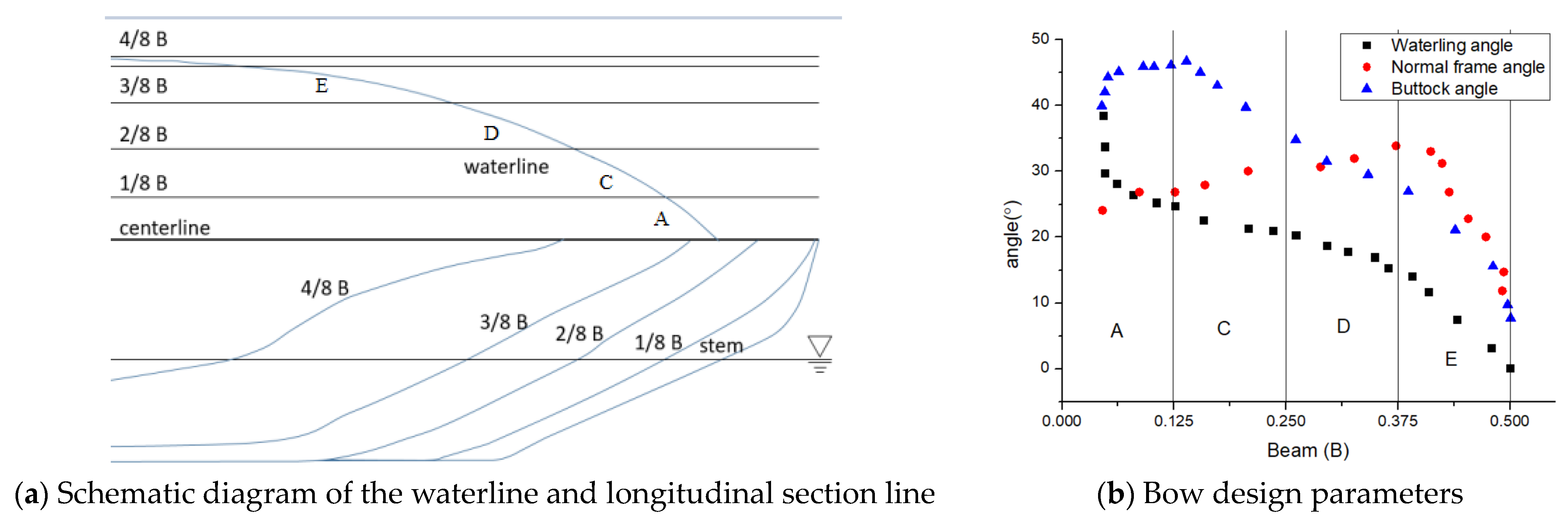
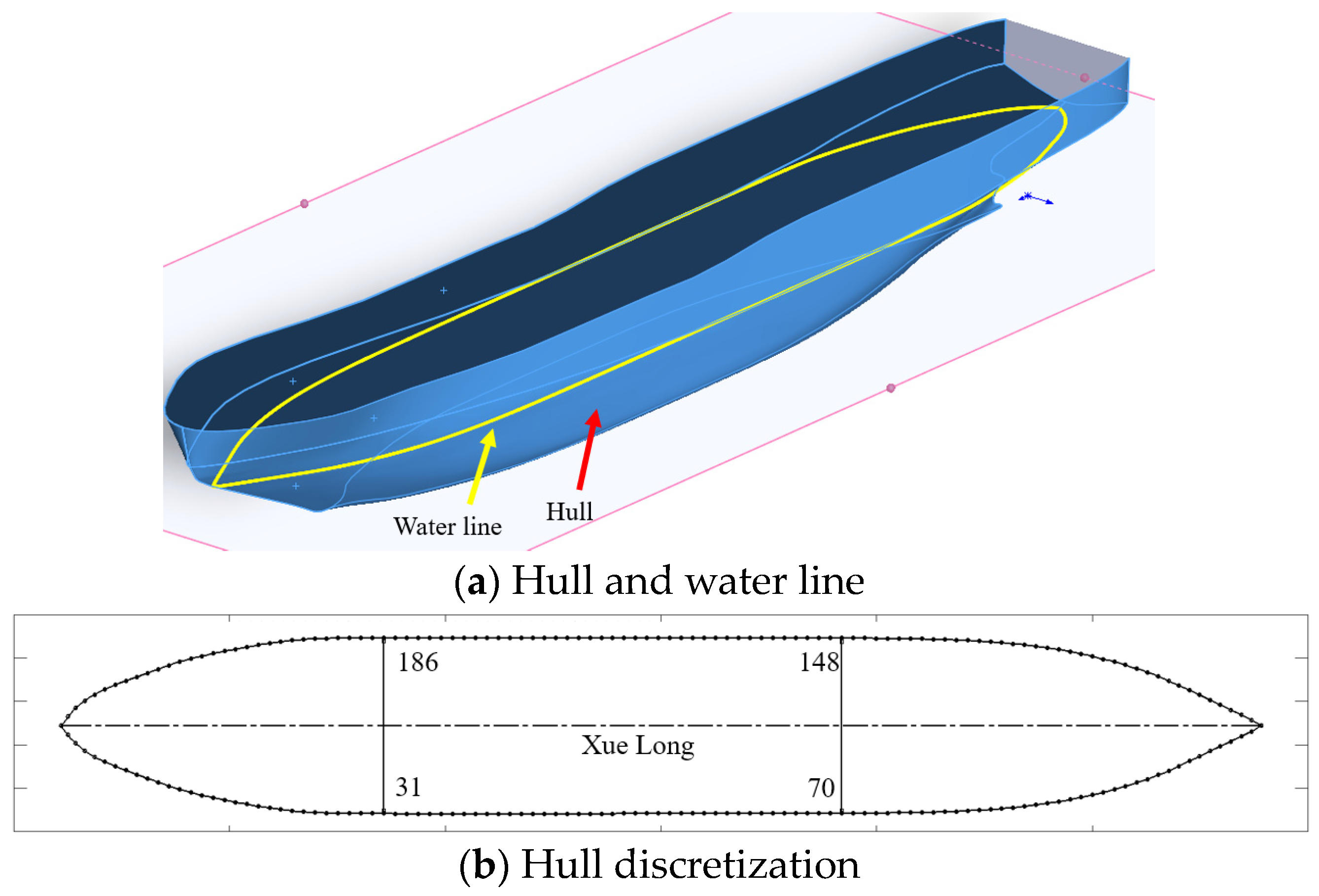
4.5. Discretization of the Ship

The number of station points on a ship significantly affects the accuracy of numerical simulation calculations. An insufficient number of points may yield inaccurate results, while an excessive number can hinder the computational efficiency. To investigate the optimal balance between accuracy and efficiency, the hull was discretized into various station counts: 137, 157, 177, 197, 217, 236, and 256. The average resistance of the ship with different station numbers was calculated, as shown in Figure 16. The black line is the average resistance, and the blue line is the calculation time. The results reveal that the hull resistance increases with the number of stations and stabilizes at 217 stations. This finding suggests that for an optimal trade-off between calculation accuracy and efficiency, the hull should be modeled with 217 stations in a two-dimensional digital ship model for subsequent numerical simulations. Figure 17 illustrates the waterplane discrete hull model of this ship.

4.6. Results

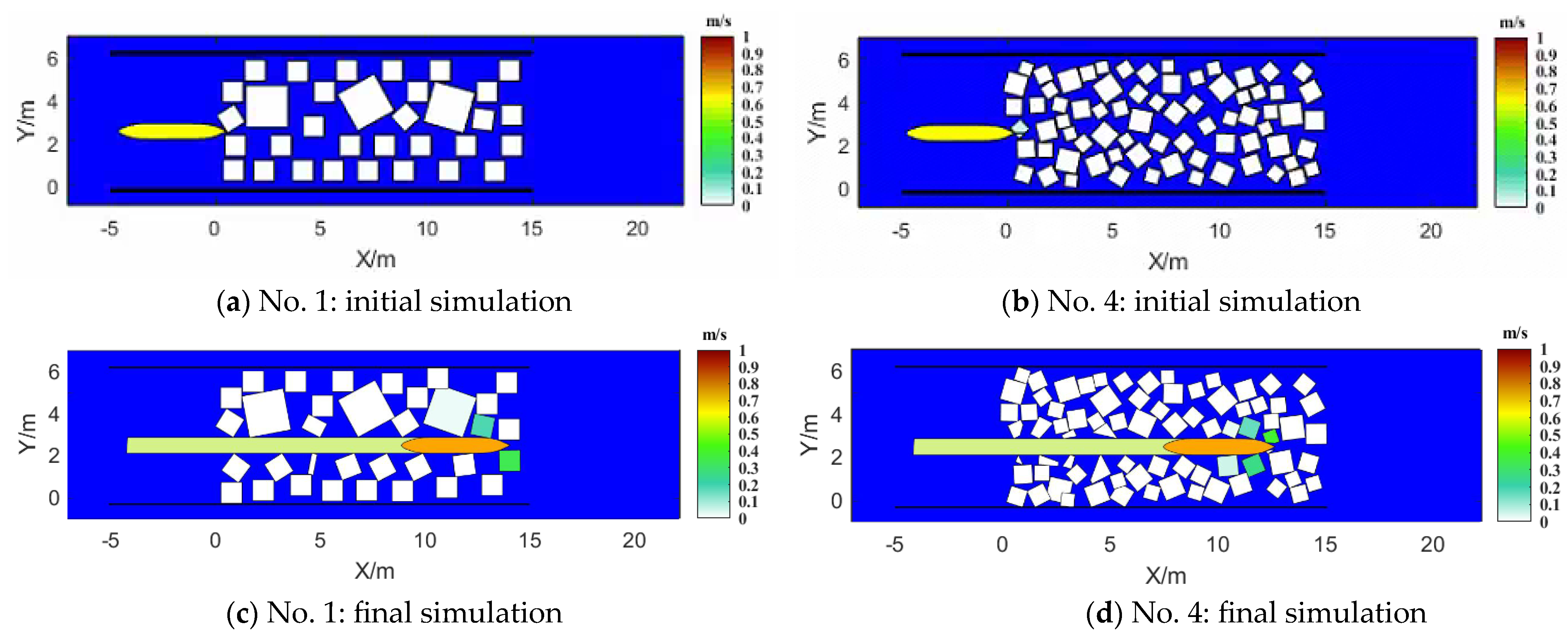
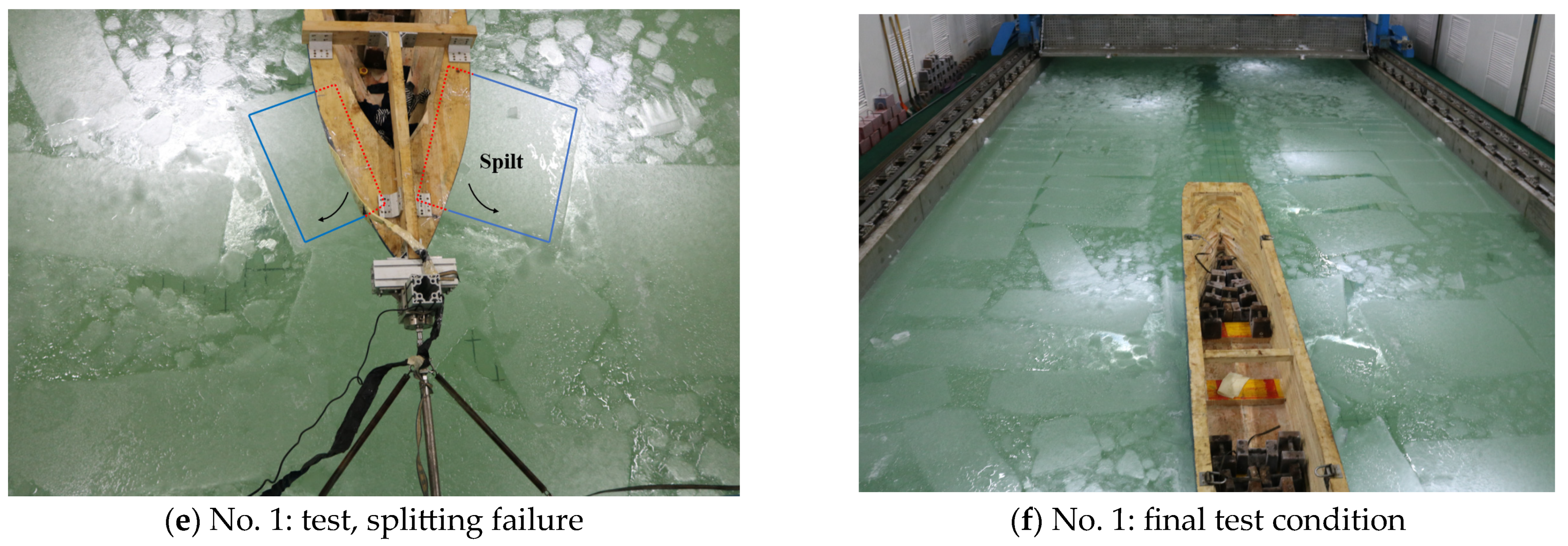
4.6.1. Comparison of Test Phenomena

Figure 18 shows the comparison between the model tests and simulations. Various failure modes were observed in the ice–ship interaction conditions. Initial contact with the bow stem can cause the ice to either split or be pushed aside and rotated alongside the ship. This phenomenon is highly consistent with the ice failure patterns and movements observed during the model test. The speed of the ice floe was also calculated in this study. Based on the velocity representation of the ice in the calculation, the mechanical transfer relationship between the ice bodies can be found.

Despite the overall agreement between the numerical simulations and the model test observations, some differences are evident, especially in terms of crack propagation paths and the final crack shapes. These differences may be attributed to the simplifying assumptions used in the numerical model, which assumes that splitting cracks advance along the initial crack line. In contrast, the ice floes in the ice tank display more complex cracking patterns, which may have been influenced by internal defects and other factors that were not incorporated into the numerical model.

There are fewer bending fracture events in the tests and simulations, but the rotational movement of the ice floes along the hull and their trajectory away from the hull after collision are similar to the test results, indicating the model’s ability to replicate dynamic interactions accurately. Notably, during model tests, when ice floes contacted the tank walls and were subsequently impacted by other floes, they could vertically overlap without resulting in failure. The displacement of ice floes after hitting the ice tank wall was constrained in the simulations.

The wake of the ship and the distribution of ice post-navigation observed in the simulations are similar to those observed in the model tests. This similarity further validates the simulation’s effectiveness in replicating real-world phenomena under controlled conditions. Numerical calculations also play a key role in capturing the velocity and detailed movements of ice floes post-collision, both between the ship and ice and among the ice floes themselves. These parameters are often challenging to measure directly in ice tank tests due to limitations in tracking and measurement technologies available in such setups. The numerical simulation of ship navigation in ice-covered waters significantly extends and enhances the capabilities of traditional ice tank tests.

4.6.2. Comparison of Resistance Time History and Average Resistance

This study presents a robust method for comparing the validity and accuracy of the simulation and test results by verifying numerical models with resistance time histories. Figure 19 shows the resistance time history curves of test data and numerical simulations under the same conditions. The overall trends, fluctuation frequencies, and average resistance values of the numerical simulations are similar to those observed in the model tests, indicating that the numerical simulations can successfully replicate the model tests. It is found that when the sailing speed increases, the resistance also increases. At the same speed, the higher the concentration, the greater the navigation resistance. In addition, it can be observed that both the simulation results and the test results occur an irregular periodic fluctuation. This phenomenon is attributed to the random collisions with single ice floes during the interaction between the ship and the ice floes. This indicates that the numerical method developed in this paper is capable of effectively simulating the crucial collision process of ship–ice collisions as observed in the test.

Despite their significant similarity, discrepancies appear in the magnitudes of maximal and minimal forces and the oscillatory behavior. The differences in the maximal and minimal forces may be attributed to simplified assumptions regarding ice properties or interaction dynamics. Numerical models that assume that ships maintain a constant forward speed might oversimplify the dynamic interactions and influence the calculations. Such constraints differ from the experimental setup, which allows for greater freedom in roll and yaw motions, potentially resulting in a more complex interaction dynamic that the model does not fully simulate. Replicating this dynamic precisely in a numerical model is challenging, as the conditions in the model are more controlled.

The interaction dynamics between the ship and ice in the numerical simulations are very similar to those observed in the model tests. Figure 20a illustrates this comparison by presenting the error ratio of the average resistance obtained from each set of tests and numerical simulations. It can be observed that under low concentration conditions, the numerical calculation results tend to be higher than the test results. Conversely, under high concentration conditions, the numerical calculation results are generally lower than those obtained experimentally. Moreover, it is evident that the overall variation trend is consistent with the changes in the working conditions. And it can be found that the error between the two is relatively small. In order to quantitatively describe the error between the simulation and model test, the relative error is defined as follows:

$$Error={\displaystyle \frac{\left|{\mathrm{R}}_{sim}-R_{test}\right|}{R_{test}}}$$

(52)

Figure 20b shows that the error values vary from 0.01692 to 0.15973, with an average error rate of 0.0905. Some samples show lower errors, indicating high consistency with the test outcomes, while the dispersion in error values across different samples suggests variability in the model’s predictive accuracy. Some conditions show higher error values, such as No. 2 and No. 3. On the one hand, this error is caused by the difference between the distribution form of the pack ice in the simulation and that in the test. On the other hand, the ice shape in the numerical simulation is simplified into a square, while the ice shape in the test is more complicated and irregular. In addition, there are many small-sized broken ice pieces in the test, as shown in Figure 15. However, the broken ice model is not built into the numerical simulation, which may cause the test resistance to be greater than that of the numerical simulation. With the increase in speed, the proportion of influence of large-size ice floes on the resistance gradually increases, and the influence of small-sized broken ice gradually decreases, showing a trend of increasing error. Despite the discrepancies, an average error of 0.0905 is generally considered acceptable in complex dynamic simulations such as ship navigation in ice.

5. Conclusions

This study developed a numerical simulation method for predicting the resistance of a ship navigating in pack ice and verified it based on an ice tank test. The main conclusions are as follows:

(1)

A theory used to identify the splitting fracture and bending failure of ice was developed. The initiation of a crack is determined by whether the transverse stress is greater than the bending strength. The extension process of the crack is derived based on LFEMs. The criterion for splitting failure is defined as whether a crack propagates to 14.5% of the length of the ice. The criterion for bending failure is defined as whether maximum principal stress is larger than the bending strength.

(2)

The kinematics of ice were derived, and a collision detection algorithm was developed based on the SAP and GLK algorithms. Closed-form solutions for the stress distribution of ice were calculated based on Symplectic Mechanics and Hooke’s law. A program for predicting the resistance of ship navigation in pack ice was developed and the theories mentioned above.

(3)

A series of model tests were conducted in an ice tank to validate the numerical simulations. Comparisons between the numerical simulations and the model tests demonstrated that the numerical simulations accurately replicated the observed interactions between the ship and ice. The ice failure modes of sliding, splitting, and bending observed in the simulations closely matched those in the model tests. The total discrepancy between the calculated average navigation resistance and the resistance observed in the model tests was 9.05%.

It is worth pointing out that this study is the first and most fundamental step of our research as a whole. We would like to develop a novel method for simulating ship navigation in pack ice. This study developed the ice failure theory, ice load calculation theory, and simulation program. However, there are some issues that need further research. For example, the square ice floes used in this study were chosen based on the consideration of stress calculations, but they cannot accurately replicate the irregular shape observed in tests. Additionally, the influence of a random ice floe distribution on resistance has not been sufficiently investigated, and the impact of ship–ice interaction on the hull remains a key focus for future research. This study serves as initial research to validate the most fundamental method underpinning this theory, thereby providing a crucial theoretical foundation for subsequent studies. Further research on these issues is currently being carried out, and related research results will be published in the future if breakthroughs are achieved.

References

1. Huang, Y.; Sun, C.; Sun, J. Route Planning of a Polar Cruise Ship Based on the Experimental Prediction of Propulsion Performance in Ice. J. Mar.Sci. Eng. 2023, 11, 1655. [Google Scholar] [CrossRef]
2. Yang, B.; Zhang, G.; Rao, H.; Wang, S.; Yang, B.; Sun, Z. Numerical simulation of the maneuvering performance of ships in broken ice area. Ocean Eng. 2024, 294, 116783. [Google Scholar] [CrossRef]
3. Li, F.; Huang, L. A Review of Computational Simulation Methods for a Ship Advancing in Broken Ice. J. Mar. Sci. Eng. 2022, 10, 165. [Google Scholar] [CrossRef]
4. Zhong, K.; Ni, B.-Y.; Li, Z. Direct measurements and CFD simulations on ice-induced hull pressure of a ship in floe ice fields. Ocean Engineering. 2023, 272, 113523. [Google Scholar] [CrossRef]
5. Tang, X.; Zou, M.; Zou, Z.; Li, Z.; Zou, L. A parametric study on the ice resistance of a ship sailing in pack ice based on CFD-DEM method. Ocean Eng. 2022, 265, 112563. [Google Scholar] [CrossRef]
6. Yang, B.; Sun, Z.; Zhang, G.; Yang, B.; Lubbad, R. Non-smooth discrete element method analysis of channel width’s effect on ice resistance in broken ice field. Ocean Eng. 2024, 313, 119419. [Google Scholar] [CrossRef]
7. Kim, J.; Yoon, D.H.; Choung, J. Numerical study of ship hydrodynamics on ice resistance during ice sheet breaking. Ocean Engineering. 2024, 308, 118285. [Google Scholar] [CrossRef]
8. Zou, M.; Tang, X.-J.; Zou, L.; Zou, Z.-J.; Zhang, X.-S. Numerical investigations of the restriction effects on a ship navigating in pack-ice channel. Ocean Eng. 2024, 305, 117968. [Google Scholar] [CrossRef]
9. Daley, C. IACS Unified Requirements for Polar Ships Background Notes to Design Ice Loads. June 2000. Available online: https://www.engr.mun.ca/~cdaley/9093/PC_Ship-Ice%20Loads.pdf. (accessed on 1 October 2024).
10. Daley, C. IACS Unified Requirements for Polar Ships Background Notes to Longitudinal Strength. 31 May 2000. Available online: https://www.engr.mun.ca/~cdaley/9093/PC_S_LONGL.pdf. (accessed on 1 October 2024).
11. ISO 19906; Petroleum and Natural Gas Industries—Arctic Offshore Structures. ISO: Geneva, Switzerland, 2019.
12. Su, B.; Riska, K.; Moan, T. A numerical method for the prediction of ship performance in level ice. Cold Reg. Sci. Technol. 2010, 60, 177–188. [Google Scholar] [CrossRef]
13. van den Berg, M.; Lubbad, R.; Løset, S. An implicit time-stepping scheme and an improved contact model for ice structure interaction simulations. Cold Reg. Sci. Technol. 2018, 155, 193–213. [Google Scholar] [CrossRef]
14. Sawamura, J. 2D numerical modeling of icebreaker advancing in ice-covered water. Int. J. Nav. Archit. Ocean. Eng. 2018, 10, 385–392. [Google Scholar] [CrossRef]
15. Lu, W.; Lubbad, R.; Løset, S. Out-of-plane failure of an ice floe: Radial-crack initiation-controlled fracture. Cold Regions Science and Technology. 2015, 119, 183–203. [Google Scholar] [CrossRef]
16. Masterson, D.M.; Frederking, R.M.W.; Wright, B.; Kärnä, T.; Maddock, W.P. A revised ice pressure–area curve. In Proceedings of the 19th International Conference on Port and Ocean Engineering under Arctic Conditions, Dalian, China, 27–30 June 2007; Volume 1, pp. 305–314. [Google Scholar]
17. Sun, J.; Huang, Y. Investigations on the ship-ice impact: Part 1. Experimental methodologies. Mar. Struct. 2020, 72, 102772. [Google Scholar] [CrossRef]
18. Lubbad, R.; Løset, S. A numerical model for real-time simulation of ship–ice interaction. Cold Reg. Sci. Technol. 2011, 65, 111–127. [Google Scholar] [CrossRef]
19. Lu, W.; Lubbad, R.; Løset, S. In-plane fracture of an ice floe: A theoretical study on the splitting failure mode. Cold Reg. Sci. Technol. 2015, 110, 77–101. [Google Scholar] [CrossRef]
20. Kim, E.; Lu, W.; Lubbad, R.; Løset, S.; Amdahl, J. Toward a holistic load model for structures in broken ice. In Proceedings of the 23rd International Conference on Port and Ocean Engineering under Arctic Conditions, Trondheim, Norway, 14–18 June 2015. [Google Scholar]
21. Li, R.; Zhong, Y.; Li, M. Analytic bending solutions of free rectangular thin plates resting on elastic foundations by a new symplectic superposition method. Proc. R. Soc. A 2013, 469, 20120681. [Google Scholar] [CrossRef]
22. Lindqvist, G. A straightforward method for calculation of ice resistance of ships. In Proceedings of the 10th International Conference on Port and Ocean Engineering under Arctic Conditions, Lulea, Sweden, 12–16 June 1989; pp. 722–735. [Google Scholar]
23. Valanto, P. The resistance of ships in level ice. SNAME Trans. 2001, 109, 53–83. [Google Scholar]
24. Lamb, H. Hydrodynamics; Cambridge University Press: Cambridge, UK, 1995. [Google Scholar]
25. Zong, Z.; Zhou, L. A theoretical investigation of ship ice resistance in waters covered with ice floes. Ocean Eng. 2019, 186, 106114. [Google Scholar] [CrossRef]
26. Hetényi, M. Beams on Elastic Foundation, 1st ed.; University of Michigan Press: Ann Arbor, MI, USA, 1946. [Google Scholar]
27. Kerr, A.D. The bearing capacity of floating ice plates subjected to static or quasi-static loads. J. Glaciol. 1976, 17, 76. [Google Scholar]
28. Nevel, D.E. Bending and Buckling of a Wedge on an Elastic Foundation. In Physics and Mechanics of Ice; Springer: Berlin/Heidelberg, Germany, 1980. [Google Scholar]
29. Paavilainen, J.; Tuhkuri, J.; Polojärvi, A. 2D combined finite-discrete element method to model multi-fracture of beam structures. Eng. Comput. 2009, 26, 578–598. [Google Scholar] [CrossRef]
30. Bhat, S.U. Analysis for splitting of ice floes during summer impact. Cold Reg. Sci. Technol. 1988, 15, 53–63. [Google Scholar] [CrossRef]
31. Bhat, S.U.; Choi, S.K.; Wierzbicki, T.; Karr, D.G. Failure analysis of impacting ice floes. J. Offshore Mech. Arct. Eng. 1991, 113, 171. [Google Scholar] [CrossRef]
32. Wang, S.; Dempsey, J.P. A cohesive edge crack. Eng. Fract. Mech. 2011, 78, 1353–1373. [Google Scholar] [CrossRef]
33. Wang, Y.; Poh, L.H. Initial-contact-induced bending failure of a semi-infinite ice sheet with a radial-before-circumferential-crack pattern. Cold Reg. Sci. Technol. 2019, 168, 102866. [Google Scholar] [CrossRef]
34. Wu, X.R. A review and verification of analytical weight function methods in fracture mechanics. Fatigue Fract. Eng. Mater. Struct. 2019, 42, 2017–2042. [Google Scholar] [CrossRef]
35. Wu, X.-R.; Xu, W. Weight Function Methods in Fracture Mechanics; Springer: Singapore, 2022. [Google Scholar]
36. Tada, H.; Paris, P.C.; Irwin, G.R. The Stress Analysis of Cracks Handbook 130; ASME Press: New York, NY, USA, 2000. [Google Scholar]
37. Ventsel, E.; Krauthammer, T. Thin Plates and Shells: Theory: Analysis, and Applications; CRC Press: New York, NY, USA, 2001. [Google Scholar]
38. Gold, L.W. Use of ice covers for transportation. Can. Geotech. J. 1971, 8, 170–181. [Google Scholar] [CrossRef]
39. Hamilton, J.; Holub, C.; Blunt, J.; Mitchell, D.; Kokkinis, T. Ice management for support of arctic floating operations. In Proceedings of the OTC Arctic Technology Conference, Houston, TX, USA, 7–9 February 2011. [Google Scholar]
40. Hoving, J.S.; Vermeulen, R.; Mesu, A.W.; Cammaert, A.B. Experiment-based relations between level ice loads and managed ice loads on an arctic jack-up structure. In Proceedings of the 22nd International Conference on Port and Ocean Engineering under Arctic Conditions, Espoo, Finland, 9–13 June 2013. [Google Scholar]
41. Yang, B. Research on Prediction Method and Influence Law of Ice Resistance of Ship in Broken Ice Conditions. Ph.D. Thesis, Dalian University of Technology, Dalian, China, 2022. [Google Scholar]
Figure 1. A logical flowchart of this study.
Jmse 12 02251 g001
Figure 2. Ice fracture scenario of a ship navigating in pack ice.
Jmse 12 02251 g002
Figure 3. Interaction modes between a ship and ice. (a). Ice rotates and slides along the hull. (b). Ice undergoes a split failure. (c). Ice slides along the shoulder of the ship. (d). Local bending failure. (e). Ice slides along the midsection of the ship.
Jmse 12 02251 g003
Figure 4. Interaction process between the ship shoulder and ice: (a) the ice thickness is not penetrated; (b) the ice thickness is penetrated.
Jmse 12 02251 g004
Figure 5. Definition of hull angles.
Jmse 12 02251 g005
Figure 6. Force analysis between the ship and ice.
Jmse 12 02251 g006
Figure 7. A finite rectangular thin plate on a Winkler elastic foundation.
Jmse 12 02251 g007
Figure 8. Boundary decomposition and superposition.
Jmse 12 02251 g008
Figure 9. Collision process between the ship and ice at different time steps.
Jmse 12 02251 g009
Figure 10. Schematic diagram of the SAP algorithm [41].
Jmse 12 02251 g010
Figure 11. Schematic diagram of the Minkowski sum.
Jmse 12 02251 g011
Figure 12. Flowchart of the numerical simulation.
Jmse 12 02251 g012
Figure 13. Towing test system.
Jmse 12 02251 g013
Figure 14. Test system for the mechanical parameters of the model ice.
Jmse 12 02251 g014aJmse 12 02251 g014b
Figure 15. Main parameters of RV Xue Long.
Jmse 12 02251 g015
Figure 16. Average resistance and simulation time for different numbers of stations.
Jmse 12 02251 g016
Figure 17. Water line and idealized segmentation.
Jmse 12 02251 g017
Figure 18. Ship–ice interaction scenario in numerical simulations.
Jmse 12 02251 g018aJmse 12 02251 g018b
Figure 19. Time history of navigational resistance between the model tests and simulations.
Jmse 12 02251 g019
Figure 20. Comparison between the test and simulation data.
Jmse 12 02251 g020