Ship-Route Prediction Based on a Long Short-Term Memory Network Using Port-to-Port Trajectory Data

Abstract

In this study, a ship-route prediction model based on a long short-term memory network using port-to-port trajectory data is presented. Data from a traditional automatic identification system—often used for ship-route prediction—are limited by uneven sampling intervals and noise. To address these issues, equal-interval data collected every 10 s from a target ship, which is a liner container vessel, were employed. Our study focuses on predicting the entire trajectory between the Gunsan and Busan ports. The root mean square error (RMSE), mean absolute error (MAE), and average distance $\overline{d}$ between two trajectories were used as the key evaluation metrics. The analysis yielded excellent predictive performance, with the values RMSE = 0.000999, MAE = 0.000672, and $\overline{d}$ = 0.101 km. This study thus provides a foundation for predicting complete port-to-port routes and offers practical insights for managing vessel operations. Accurate route prediction contributes to reducing port congestion, improving fuel efficiency, and lowering carbon emissions.

1. Introduction

With the introduction of autonomous maritime surface ships, the maritime traffic environment has become significantly more complex, requiring the future development of intelligent maritime traffic networks [1]. Accordingly, technologies such as ship-route planning [2,3], safe navigation for collision prevention [4], and maritime traffic control [5,6] are required, with accurate ship-route prediction gaining attention as a crucial technology. Ship-route prediction mainly utilizes historical trajectories based on data obtained from automatic identification systems (AISs), and machine-learning and deep-learning technologies are being used for ship-trajectory prediction research [1].

An AIS is a device that exchanges information with nearby ships, stations, and satellites to identify and track the positions of vessels and other maritime traffic [7]. The AIS data contain dynamic information—such as the ship’s position, time, speed over ground (SOG), and course over ground (COG)—as well as static information, including the ship’s identifying number, type, length, width, etc. [5,7,8]. Owing to their comprehensive coverage, high sampling rates, and convenience, AIS data have become a primary source for ship-route predictions and maritime traffic analysis [1]. However, AIS data have critical limitations for predicting time-series data such as ship trajectories. According to the technical standards of the International Telecommunication Union, the transmission rate of AIS data for Class A vessels is determined based on a ship’s status and speed, which are collected at non-equal intervals, as shown in

Table 1. Transmission rates of AIS data for Class A vessels.

Ship Status and Speed	Reporting Interval
Ships anchored or moored and not moving faster than 3 knots	3 min
Ships anchored or moored and moving faster than 3 knots	10 s
Ships with speeds ranging from 0 to 14 knots	10 s
Ships with speeds ranging from 0 to 14 knots and changing course	3 1/3 s
Ships with speeds ranging from 14 to 23 knots	6 s
Ships with speeds ranging from 14 to 23 knots and changing course	2 s
Ship speed > 23 knots	2 s
Ship speed > 23 knots and changing course	2 s

[7,8]. However, it can be challenging for predictive models to learn patterns effectively from time-series data that are not collected at regular intervals [9]. Because the characteristics of ship-trajectory data are influenced by factors such as wind and water depth, irregular time intervals between data samples make it difficult to capture and incorporate correlations between the variables into a predictive model. Further, AIS data often contain noise, e.g., in the ship’s position, speed, and time stamp [10]. In addition, if the quality of the AIS equipment is low or if it is improperly installed, data-transmission errors may occur.

Due to the limitations caused by noise or transmission errors, previous studies have often handled AIS data either by cleaning erroneous data or by performing preprocessing tasks to convert nonequal-interval data into equal-interval data [11,12,13,14,15,16]. Consequently, previous studies have been limited to predicting short voyage distances on a minute-to-minute or hourly basis. In contrast, in the present study, a prediction model was developed using ship-trajectory data collected at regular 10 s intervals from a liner vessel. This approach overcomes the limitations of conventional AIS data, ensuring the stable acquisition of evenly spaced data suitable for time-series predictions. Another goal of this study is to predict the port-to-port trajectory data—which has rarely been addressed in previous research—by utilizing long-term onboard data from the liner vessel.

A liner vessel refers to a ship operated by a shipping company along fixed routes and with fixed schedules, enabling ship-owners and shippers to book it accordingly [17]. One of the critical characteristics of liner vessels is that they operate repeatedly along specific routes and must arrive at scheduled times. When ships are unable to arrive at ports on time because of port congestion, bad weather, or other factors, recovery actions become necessary, such as skipping ports or increasing speed. Such changes cause schedule delays, maritime traffic congestion, increased fuel consumption, and higher carbon emissions [18]. The approach described in the present study is thus a valuable aid for decision-making by navigation officers and engineers operating liner vessels, as it provides insights into unexpected disruptions that may arise during liner operations. In addition, by predicting the entire ship trajectory from port to port, we can improve maritime traffic safety and operational efficiency.

This study is structured around the following key aspects: First, instead of using the AIS data typically employed for ship-route prediction, we utilize equal-interval onboard data received directly from the liner vessel. Second, we propose a foundational study that predicts port-to-port trajectories rather than focusing on short distances or time frames. Third, we have developed an algorithm using a long short-term memory (LSTM) network—a recurrent neural-network model suitable for time-series data—and have utilized it to develop and select the best-performing final model.

2. Materials and Methods

Figure 1 shows a flowchart of the present study. First, we collected the ship-trajectory data sensed from the target ship. These data include the raw positional and navigational information necessary for trajectory prediction. We then clustered the data into port-to-port trajectory units. Clustering helps segment the trajectory into meaningful units for more focused and accurate analysis. We subsequently carried out preprocessing to prepare the data for use in the prediction algorithms. The preprocessing steps, including filtering data above 3 knots, interpolation, and scaling, ensure the data quality and uniformity required for effective training of the LSTM network. And, for the purpose of model training and evaluation, the dataset was divided into training and test datasets. Most of the trajectories from the collected data were used as the training dataset, while one representative trajectory was selected and designated as the test dataset. Finally, we constructed a ship-route prediction algorithm using an LSTM network, and we derived the final model using an evaluation process. This step evaluates the model’s performance to ensure its applicability and robustness in real-world ship-route prediction scenarios.

2.1. Dataset

2.1.1. Ship Trajectory

The target ship for this study is a container ship with the specifications listed in

Table 2. Target ship’s particulars.

Category	Information
Ship type	Container
Length overall (meters)	134.67
Breadth (meters)	22.6
Deadweight tonnage (metric tons)	12,512
Net tonnage (metric tons)	4959
Gross tonnage (metric tons)	9956
Propeller diameter (millimeters)	5400
Propeller pitch (millimeters)	4638
Main engine power at M.C.R * (kilowatts)	7860
Main engine power at M.C.R (round per minute)	129

* Maximum continuous rating.

. It is a liner ship sailing between ports in the Republic of Korea and China, and it calls at four ports: Busan, Gwangyang, Qingdao, and Gunsan.

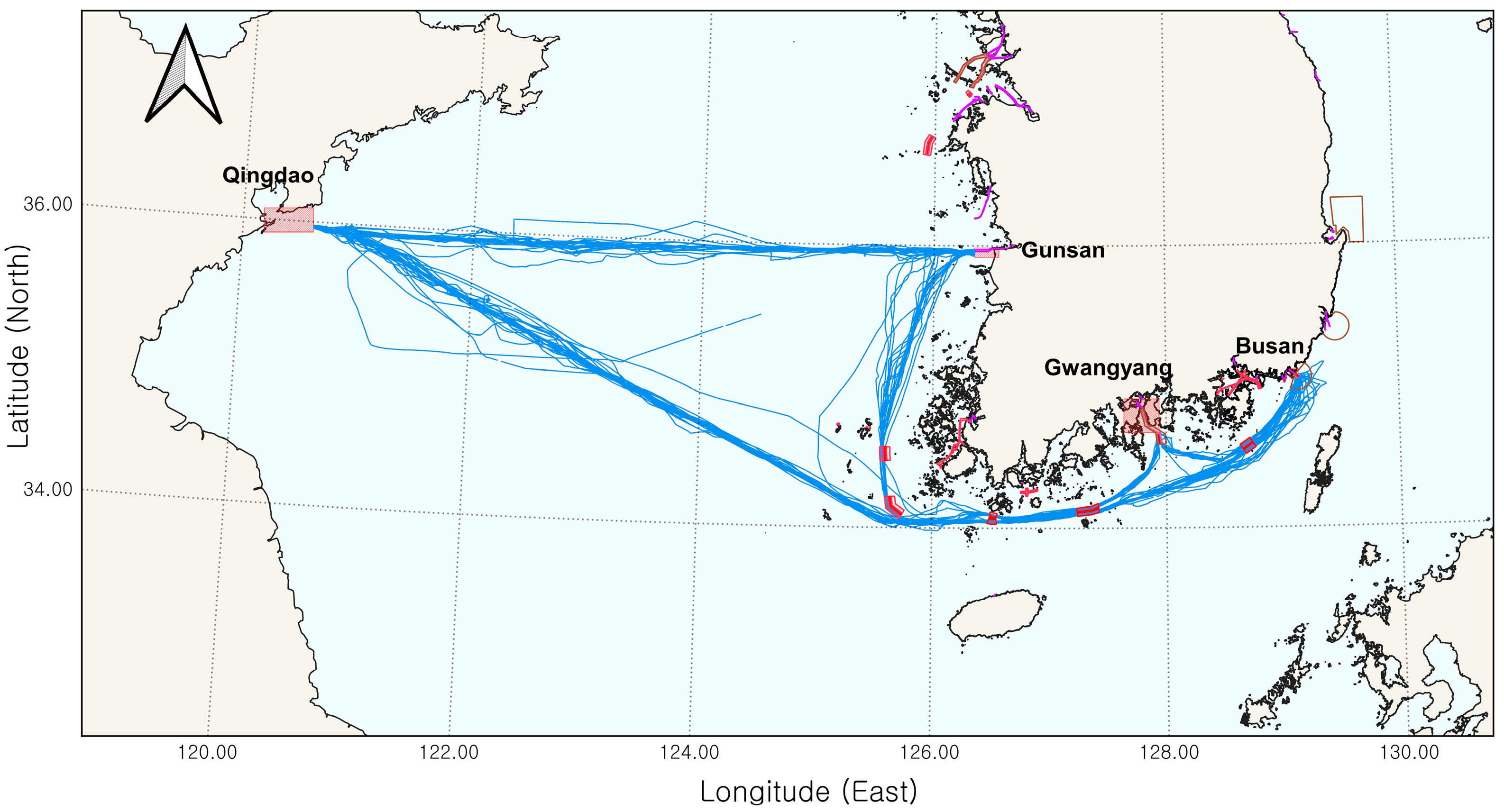
The target ship’s trajectory data were reported every 10 s from aboard the ship. We collected data for a period of 6 months, from 1 February to 31 July 2023, and the navigation period between departing from Busan and entering Busan again is about a week. Figure 2 presents a visualization of the ship-trajectory data collected for this study. These data include information such as the time stamp, latitude, longitude, SOG, transverse SOG, speed through water (STW), transverse STW, relative wind direction, absolute wind direction, COG, ship heading, water depth, rudder angle, draft, and engine data, among others. The additional data, such as wind and rudder angle, were collected using onboard sensors, which extend beyond the scope of AIS data. However, similar to models that use AIS data, in this study, we utilized only the time stamp, latitude, longitude, SOG, and COG for the analysis. This decision aligns with most previous studies [11,12,13,14,15,16] focusing on these AIS-provided variables due to their availability and proven utility in ship-route prediction models. Future research could explore including additional variables to further enhance model performance.

2.1.2. Ship-Trajectory Clustering

We classified the ship-trajectory data used in this study into port-to-port segments using a K-means clustering algorithm. The K-means clustering identifies the centroid of each cluster and assigns each data point to the nearest centroid, thereby grouping the data accordingly [19]. In this study, we vectorized the ship trajectories based on their starting points [start_latitude, start_longitude] and ending points [end_latitude, end_longitude]. Using K-means, we then grouped the vectorized trajectories into four clusters, corresponding to the segments between ports.

K-means was selected for its simplicity, computational efficiency, and effectiveness in grouping spatial data based on proximity. Given the nature of ship trajectories, which their start and end points can effectively describe, K-means provided a straightforward approach to minimize intra-cluster distances. While other clustering methods, such as DBSCAN or hierarchical clustering, could be considered, K-means was particularly suitable for this application due to the relatively small size of the dataset and the clear spatial separation of trajectory groups.

2.2. Data Preprocessing

After clustering the ship-trajectory data, we extracted only the trajectories departing from Gunsan Port and arriving at Busan Port. We focused the analysis on this route because it includes the most frequent course changes and the most complex sections of the target ship’s trajectory. We then preprocessed these extracted trajectories for use in the ship-route prediction algorithm.

First, to focus on vessels in navigation, we removed data points where the target ship was berthed, anchored, or drifting [2]. In particular, drifting scenarios often occur when the sea area is influenced by external forces such as currents or wind. These situations may result in irregular movements, including SOG exceeding 2 knots. Or, the ship reduces its speed intentionally to adjust its arrival time at the next port. As such, to ensure consistency in the analysis and focus on data corresponding to ships in operation, we excluded data points where the SOG was less than 3 knots, based on the criteria in Table 1 [8].

We employed interpolation to fill in the data gaps caused by removing these data and by missing values due to data-transmission errors. We used a linear interpolation method with a 10 s interval for consistency with the time intervals in the original dataset. Linear interpolation was selected because ship trajectories typically exhibit smooth changes in position and speed over short intervals, making this method appropriate for estimating intermediate points. Furthermore, it maintains the temporal integrity of the data without introducing additional computational complexity, which is crucial for efficient preprocessing. While other interpolation methods, such as spline or polynomial interpolation, could be considered, they may introduce unnecessary overfitting or distortions in the trajectory data.

Additionally, we scaled the data to prepare them for the ship-route prediction algorithm. In this study, we applied min–max scaling to the input variables, including the latitude, longitude, SOG, and COG data. Min–max scaling was chosen because it normalizes the variables to a consistent range, typically between 0 and 1, which prevents any single variable from dominating the training process. This step is particularly beneficial for LSTM models, as they are sensitive to the scale of input data, and normalization helps stabilize gradient calculations during optimization. By applying min–max scaling, we ensured that the input variables were treated equally, improving the overall performance and convergence of the prediction model.

2.3. Methods

In the ship-trajectory data used in this study, the position, SOG, and COG change over time. Recurrent neural networks (RNNs) are designed to process sequential information in data effectively, making them well suited for handling continuous time-series data [6,20]. However, RNNs are affected by the vanishing-gradient problem, where the memory of past data is lost over time and is not reflected in future data [20,21]. This limitation poses a significant challenge for ship-trajectory prediction, as it relies on retaining information about past movements to predict future routes accurately. To address this limitation of traditional RNNs, we designed an LSTM network with a structure that retains prior information [22]; this structure is shown in Figure 3. LSTM utilizes gated mechanisms to selectively remember or forget information, enabling them to capture long-term dependencies in sequential data. This makes them particularly suitable for ship-route prediction, where sequential dependencies, such as changes in position, speed, and direction over time, are critical for model performance.

The LSTM comprises several gates that control the long-term memory, known as the cell state ($C_t$), and the short-term memory, referred to as the hidden state ($h_t$), over time. The forget gate ($f_t$) determines which information from the previous cell state ($C_{t-1}$) should be discarded. It processes the current input ($X_t$) and the previous hidden state ($h_{t-1}$) through a sigmoid function (σ), outputting a value between 0 and 1. This value is then multiplied by the cell state to decide which information to retain or discard

$$f_t=\mathsf{\sigma }\left(W_f·\left[h_{t-1},X_t\right]+b_f\right),$$

(1)

where $W$ is weight, $b$ is the bias term added to account for data shifts and improve the flexibility of the gate, and $t$ is time. This mechanism ensures that irrelevant or outdated information is efficiently removed from the memory, allowing the model to focus on the most critical data.

The input gate ($i_t$) decides whether to add new information to the cell state. It combines a sigmoid function and a tanh function, appropriately transforming the input and reflecting it in the cell state. The new candidate information (${\widehat{C}}_t$) is calculated using the tanh function, and it is combined with the information passed through the input gate to form the new cell state ($C_t$):

$$i_t=\sigma \left(W_i·\left[h_{t-1},X_t\right]+b_i\right),$$

(2)

$${\widehat{C}}_t=tanh\left(W_c·\left[h_{t-1},X_t\right]+b_c\right), \mathrm{and}$$

(3)

$$C_t=f_t\times C_{t-1}+i_t\times {\widehat{C}}_t.$$

(4)

The input gate plays a critical role in selectively updating the cell state with new information while preserving relevant past information. This allows the model to dynamically adapt to changing input patterns.

The output gate ($o_t$) determines the next hidden state ($h_t$). It processes the current input ($X_t$) and the previous hidden state ($h_{t-1}$) through a sigmoid function to form the output gate, which is then multiplied by the cell state transformed by the tanh function to produce the final hidden state ($h_t$). This hidden state is passed on to the next LSTM cell:

$$o_t= \sigma \left(W_o·\left[h_{t-1},X_t\right]+b_o\right) \mathrm{and}$$

(5)

$$h_t=o_t\times tanh\left(C_t\right).$$

(6)

The output gate determines what portion of the cell state should be exposed as the hidden state, ensuring that only the most relevant information is passed forward. This mechanism allows the LSTM to effectively manage short-term and long-term dependencies in sequential data.

Time-series data exhibit the characteristics of continuous change over time; thus, for time-series forecasting, it is more appropriate to base predictions on recent data. Using older records to predict recent changes can be inappropriate [23]. One common practice for addressing this issue is to use the sliding-window technique. As illustrated in Figure 4, a sliding window employs a fixed-size time window and moves it continuously across the data to predict future values based on past data [24]. This approach enables the model to learn patterns that may exist between consecutive data points, allowing for more accurate forecasting of time-series trends. In this study, we set the sliding window size to 10. This size was chosen to ensure the model focuses on the most recent data while retaining enough information to capture meaningful temporal patterns, thereby optimizing the prediction accuracy.

2.4. Method for Evaluating the Model

To evaluate the accuracy of the LSTM-based ship-route prediction model proposed in this study, we compared the actual and estimated values for the ship’s $i$-th position ($pos{i}_i$). We calculated the root mean square error (RMSE) and the mean absolute error (MAE) between these two quantities as follows:

$$RMSE=\sqrt{{\displaystyle \frac{{{\displaystyle \sum }}_{i=1}^n{\left(pos{i}_i^{actual}-pos{i}_i^{estimated}\right)}^2}{n}}} \mathrm{and}$$

(7)

$$MAE={\displaystyle \frac{1}{n}}{{\displaystyle \sum }}_{i=1}^n\left|pos{i}_i^{actual}-pos{i}_i^{estimated}\right|.$$

(8)

RMSE and MAE were chosen because they effectively quantify the prediction error in continuous data, making them particularly suitable for evaluating time-series models like LSTM. RMSE emphasizes larger errors due to its quadratic nature, providing insight into significant deviations in predictions, while MAE provides an average measure of absolute errors, offering a more intuitive understanding of overall prediction accuracy.

In addition, we evaluated the accuracy of the ship-route prediction model by calculating the average actual distance between $pos{i}_i^{actual}$ and $pos{i}_i^{estimated}$ using the haversine distance formula [25]:

$$haversine\theta =si{n}^2\left({\displaystyle \frac{\theta }{2}}\right).$$

(9)

The differences between the actual and predicted values of the latitude and longitude are $\Delta lat=\left(la{t}_i^{actual}-la{t}_i^{estimated}\right)$ and $\Delta long=\left(lon{g}_i^{actual}-lon{g}_i^{estimated}\right)$, and we converted these differences into radians. In addition, we calculated a quantity a using the haversine function based on $\Delta lat$ and $\Delta long$:

$$a=haversine\Delta lat+cos\left(la{t}_i^{estimated}\right)\cos \left(la{t}_i^{actual}\right)\mathrm{haversine}\Delta long.$$

(10)

Using this quantity, we calculated central angle c, which represents the angle between two points at the center of the spherical Earth:

$$c=2·\mathrm{atan}2\left(\sqrt{a},\sqrt{1-a}\right)$$

(11)

With $R$ representing the radius of the Earth, we obtained the final distance $d$ by multiplying the central angle $c$ by $R$, as shown in Equation (12):

$$\begin{gathered} d=R·c=2r· \\ arcsin\sqrt{si{n}^2\left({\displaystyle \frac{\Delta lat}{2}}\right)+cos\left(la{t}_i^{estimated}\right)\cos \left(la{t}_i^{actual}\right)si{n}^2\left({\displaystyle \frac{\Delta long}{2}}\right)}. \end{gathered}$$

(12)

The average actual distance used as an evaluation metric in this study is then defined as follows:

$$\overline{d}={\displaystyle \frac{1}{n}}{{\displaystyle \sum }}_{i=1}^n{d}_i.$$

(13)

The haversine distance formula was selected to measure geospatial errors, which are critical for understanding the practical implications of the model’s predictions in real-world navigation scenarios. By providing a direct measurement of the distance between predicted and actual positions on a spherical Earth, this metric complements RMSE and MAE, ensuring a comprehensive evaluation of the model’s performance.

3. Results

3.1. Results of Trajectory Clustering and Interpolation

In this study, we employed K-means clustering to classify the trajectories of the target ship, which periodically sails the route Busan–Gwangyang–Qingdao–Gunsan, into port-to-port segments. We divided the trajectories into the four clusters shown in Figure 5.

Among the four ship-trajectory segments shown in Figure 5, we designated the Gunsan–Busan route the target trajectory. This route was selected due to its frequent course changes and navigational complexities, including varying traffic densities and environmental conditions. These features make it a suitable case for testing the robustness and accuracy of the prediction model, as they introduce realistic challenges that a ship might encounter during actual operations. By focusing on this route, we aimed to ensure that the model could handle complex trajectories effectively, which is essential for its practical applicability to other maritime scenarios. It consists of 24 voyages, with 23 used as training data and one as test data. To align with the scheduling of the destination port (Busan Port), we excluded data with SOG < 3 knots, which correspond to periods in which the ship was drifting, anchored, or reducing speed. To address the gaps resulting from these exclusions, we used linear interpolation to provide interpolated data at the same 10 s intervals. The results are shown in Figure 6. A comparison between the raw data before excluding SOG < 3 knots and the data after exclusion is provided in Figure A1. We also extracted the latitude, longitude, SOG, and COG data as input variables for the ship-route prediction algorithm and applied min–max scaling to them.

3.2. Evaluation of Ship-Route Prediction Models

In this study, we utilized an LSTM network to develop ship-route prediction models. To compare the performance of different models, we designated seven models for experimentation. We tested these models under the same hyperparameter settings, including a window size of 10, an epoch size of 20, and a batch size of 32. Additionally, we used the adaptive-moment-estimation (Adam) optimizer to minimize the loss function. The rationale for selecting these hyperparameters, based on a grid search, and additional experiments on sliding-window steps, is detailed in Appendix B.

The seven models are the following:

• Model 1: Basic ship-route prediction model that excludes SOG < 3 knots data;
• Model 2: Model 1 with the addition of a time-difference variable;
• Model 3: Ship-route prediction model using the interpolated training data;
• Model 4: Model 3 with a sliding-window step of 2;
• Model 5: Model 3 with prediction 20 s ahead;
• Model 6: Model 3 with prediction 30 s ahead;
• Model 7: Model 3 with prediction 60 s ahead.

We used the RMSE, MAE, and $\overline{d}$ to evaluate the performance of each model, and the experimental results are shown in

Table 3. The experimental results of ship-route prediction models.

Model	RMSE	MAE	$\overline{\mathit{d}}$ (km *)
1	0.002851	0.001730	0.265459
2	0.017656	0.011007	1.811709
3	0.000999	0.000672	0.101036
4	0.002440	0.001729	0.272371
5	0.003508	0.001938	0.292881
6	0.002380	0.001402	0.217426
7	0.038665	0.021802	3.262413

* Kilometers.

. Model 1 exhibits relatively good prediction performance even without interpolation, with a low RMSE (0.002851), MAE (0.001730), and $\overline{d}$ = 0.265 km. The time-difference variable in Model 2 represents the time interval between the timestamp of the current data point and the previous data point, capturing variations in the original dataset’s temporal spacing. Model 2 has higher values of RMSE and MAE than Model 1, indicating that adding the time-difference variable resulted in reduced accuracy. Model 3 achieved the best performance, with the lowest RMSE (0.000999), MAE (0.000672), and $\overline{d}$ = 0.101 km, demonstrating that using interpolated training data significantly improved the prediction accuracy. Model 4 yields a slightly lower performance than Model 3, with slightly higher values of RMSE and MAE, indicating that setting the window step to 2 impacted the results. Models 5 and 6 predicted 20 s and 30 s ahead, respectively, with Model 6 achieving better accuracy, as reflected by its smaller $\overline{d}$ (0.217 km vs. 0.293 km). Model 7, which predicts 60 s ahead, exhibits the highest RMSE (0.038665) and MAE (0.021802), with $\overline{d}$ = 3.262 km, showing that the accuracy decreases as the prediction interval increases.

Using Model 3, the most accurate model, we identified which segments were well-predicted and which showed significant errors during the prediction of the Gunsan–Busan route. Figure 7 compares the actual ship trajectory for the test data (green points) with the trajectory predicted by Model 3 (red points). The enlarged sections highlight the early trajectory after departing from Gunsan Port, the segment passing through the traffic-separation scheme near Maenggol Gundo, a segment with deleted data, and the section just before entering Busan Port. In some areas, there are discrepancies between the actual and predicted routes, with particularly noticeable deviations near the complex areas around Busan Port. A focused visualization showing the predicted points connected to form a curve is provided in Figure A2, highlighting a zoomed-in portion of the trajectory for better clarity. Figure 8 shows the point-wise distance differences between the test data and the predictions made by Model 3, normalized by the ship’s length (134.67 m). The x-axis represents the time step (index), and the y-axis indicates the ratio of the distance difference to the ship’s length. While the prediction error is somewhat large in the early stages, it stabilizes to less than 1 during the middle segment. However, the error increases again toward the end, reaching a maximum ratio of over 5 near time step 8000, just before arriving at Busan Port.

4. Discussion

The LSTM-based ship-route prediction model developed in this study demonstrated stable performance in experiments conducted on the Gunsan–Busan route. In particular, Model 3, which utilized the interpolated training data, exhibited the best predictive performance, achieving the lowest values of RMSE and MAE. Previous studies [7,8,9,11,12,13,14,15,16,26] have shown that the uneven collection intervals of AIS data and data noise are key challenges that negatively affect the accuracy of prediction models. The present study effectively addresses these issues by utilizing evenly spaced onboard sensor data collected at 10 s intervals, thus avoiding this limitation of AIS data and enabling more accurate time-series predictions.

Unlike previous studies [11,12,13,14,15,16], which have focused primarily on short-distance ship-route predictions, the present study provides a foundation for predicting complete ship trajectories from port to port. These results offer valuable input for the management and decision-making processes involved in liner vessel operations, as accurate route predictions can contribute to reducing port congestion, improving fuel efficiency, and lowering carbon emissions.

Additionally, we found that the prediction errors increase significantly just before entering a port. This observation aligns with the findings of Ogura et al. [27], which indicated that environmental factors, such as maritime traffic congestion and sudden weather changes, are major contributors to reduced prediction accuracy near ports. This suggests that future models should integrate dynamic environmental data, such as real-time traffic density or weather conditions, to mitigate these issues.

The results revealed that the model performed slightly better for 30 s predictions than for 20 s predictions, which can be attributed to the inherent variability in ship trajectories and the temporal dependencies captured by the LSTM model. Slightly longer intervals may provide smoother trajectory patterns, improving short-term prediction accuracy. However, prediction accuracy decreased significantly for 60 s intervals, highlighting the limitations of the current architecture for long-term forecasting. To address the reduced accuracy of long-term predictions, future research should explore advanced models, such as attention mechanisms or hybrid architectures, which are better suited for retaining relevant information over extended periods. Additionally, incorporating environmental variables, such as wind and water depth, and comparing the performance of other RNN architectures, such as gated recurrent units or attention-based models, could further enhance the predictive capability of ship-route models.

By comparing our results with the existing literature, this study highlights the importance of using evenly spaced onboard sensor data. This study lays the groundwork for extending ship-route prediction research to larger datasets and more diverse operational scenarios.

5. Conclusions

This study developed LSTM-based ship-route prediction models and evaluated them using liner vessel trajectory data collected at 10 s intervals. By addressing the challenges posed by uneven data-collection intervals and noise in traditional AIS data, the proposed approach demonstrates the potential for enhancing the accuracy of ship-trajectory time-series predictions.

The results show that Model 3, which uses interpolated data, achieved the best performance, highlighting the importance of evenly spaced training data. Furthermore, the focus on predicting entire port-to-port routes provides a foundation for improving operational efficiency in maritime transportation, with potential applications such as reducing port congestion, optimizing fuel consumption, and lowering carbon emissions.

However, this study has some limitations. Prediction errors increased near ports due to complex routing, schedule adjustments, and environmental factors. This is likely because the model relies on interpolated data at consistent intervals, which may not fully capture the irregularities and complexities of real-world AIS data. For instance, AIS data often exhibit irregular intervals due to varying reporting frequencies, and environmental factors such as weather and maritime traffic further complicate predictions. Additionally, the model’s performance decreased for longer prediction intervals. Future research should address these challenges by developing algorithms tailored for ship movements near ports, where environmental disturbances, such as maritime traffic, water depth, and weather conditions, significantly affect predictions. Incorporating such environmental variables could provide more accurate forecasts in these complex areas.

Furthermore, future work should explore advanced RNN architectures to improve predictive accuracy and investigate strategies to minimize performance degradation over longer prediction intervals. In particular, adapting the model to handle raw AIS data with irregular intervals and integrating real-time environmental data could enhance its robustness and practical applicability. Evaluating the model under diverse maritime conditions and routes would further demonstrate its adaptability and generalizability. Moreover, a comparative analysis of AIS data and onboard sensor data could further validate the model’s robustness.

The findings of this study have the potential to be applied to various routes and vessel types, contributing to the advancement of maritime traffic safety and operational efficiency.

References

- Bi, J.; Cheng, H.; Zhang, W.; Bao, K.; Wang, P. Artificial intelligence in ship trajectory prediction. J. Mar. Sci. Eng. 2024, 12, 769. [Google Scholar] [CrossRef]
- Lee, H.-T.; Choi, H.-M.; Lee, J.-S.; Yang, H.; Cho, I.-S. Generation of ship’s passage plan using data-driven shortest path algorithms. IEEE Access. 2022, 10, 126217–126231. [Google Scholar] [CrossRef]
- Lee, H.-T.; Kim, M.-K. Optimal path planning for a ship in coastal waters with deep Q network. Ocean Eng. 2024, 307, 118193. [Google Scholar] [CrossRef]
- Abebe, M.; Noh, Y.; Kang, Y.-J.; Seo, C.; Kim, D.; Seo, J. Ship trajectory planning for collision avoidance using hybrid ARIMA-LSTM models. Ocean Eng. 2022, 256, 111527. [Google Scholar] [CrossRef]
- Lee, J.-S.; Kim, T.-H.; Park, Y.-G. Maritime Transport Network in Korea: Spatial-Temporal Density and Path Planning. J. Mar. Sci. Eng. 2023, 11, 2364. [Google Scholar] [CrossRef]
- Shin, G.-H.; Yang, H. Vessel trajectory prediction at inner harbor based on deep learning using AIS data. J. Mar. Sci. Eng. 2024, 12, 1739. [Google Scholar] [CrossRef]
- Lee, H.-T.; Lee, J.-S.; Yang, H.; Cho, I.-S. An AIS data-driven approach to analyze the pattern of ship trajectories in ports using the DBSCAN algorithm. Appl. Sci. 2021, 11, 799. [Google Scholar] [CrossRef]
- Kim, H.-C.; Son, W.-J.; Lee, J.-S.; Cho, I.-S. Identification of maritime areas with high vessel traffic based on polygon shape similarity. IEEE Access 2024, 12, 92253–92267. [Google Scholar] [CrossRef]
- Liu, X.; Du, H.; Yu, J. A forecasting method for nonequal-interval time series based on recurrent neural network. Neurocomputing 2023, 556, 126648. [Google Scholar] [CrossRef]
- Emmens, T.; Amrit, C.; Abdi, A.; Ghosh, M. The promises and perils of automatic identification system data. Expert Syst. Appl. 2021, 178, 114975. [Google Scholar] [CrossRef]
- Tang, H.; Yin, Y.; Shen, H. A model for vessel trajectory prediction based on long short-term memory neural network. J. Mar. Eng. Technol. 2022, 21, 136–145. [Google Scholar] [CrossRef]
- Murray, B.; Perera, L.P. An AIS-based deep learning framework for regional ship behavior prediction. Reliab. Eng. Syst. Saf. 2021, 215, 107819. [Google Scholar] [CrossRef]
- Qian, L.; Zheng, Y.; Li, L.; Ma, Y.; Zhou, C.; Zhang, D. A new method of inland water ship trajectory prediction based on long short-term memory network optimized by genetic algorithm. Appl. Sci. 2022, 12, 4073. [Google Scholar] [CrossRef]
- Wang, S.; Li, Y.; Xing, H. A novel method for ship trajectory prediction in complex scenarios based on the spatio-temporal feature extraction of AIS data. Ocean Eng. 2023, 281, 114846. [Google Scholar] [CrossRef]
- Venskus, J.; Treigys, P.; Markevičiūtė, J. Unsupervised marine vessel trajectory prediction using the LSTM network and wild bootstrapping techniques. Nonlinear Anal. Model. Control 2021, 26, 718–737. [Google Scholar] [CrossRef]
- Gao, D.W.; Zhu, Y.S.; Zhang, J.F.; He, Y.K.; Yan, K.; Yan, B.R. A novel MP-LSTM method for ship trajectory prediction based on AIS data. Ocean Eng. 2021, 228, 108956. [Google Scholar] [CrossRef]
- Dulebenets, M.A.; Pasha, J.; Abioye, O.F.; Kavoosi, M. Vessel scheduling in liner shipping: A critical literature review and future research needs. Flex Serv. Manuf. J. 2021, 33, 43–106. [Google Scholar] [CrossRef]
- Asghari, M.; Jaber, M.Y.; Mirzapour Al-e-Hashem, S.M.J. Coordinating vessel recovery actions: Analysis of disruption management in a liner shipping service. Eur. J. Oper. Res. 2023, 307, 627–644. [Google Scholar] [CrossRef]
- Son, W.-J.; Cho, I.-S. Analysis of Trends in Mega-Sized Container Ships Using the K-Means Clustering Algorithm. Appl. Sci. 2022, 12, 2115. [Google Scholar] [CrossRef]
- Tian, X.; Suo, Y. Research on Ship Trajectory Prediction Method Based on Difference Long Short-Term Memory. J. Mar. Sci. Eng. 2023, 11, 1731. [Google Scholar] [CrossRef]
- Bengio, Y.; Simard, P.; Frasconi, P. Learning long-term dependencies with gradient descent is difficult. IEEE Trans. Neural Netw. 1994, 5, 157–166. [Google Scholar] [CrossRef] [PubMed]
- Hochreiter, S.; Schmidhuber, J. Long short-term memory. Neural Comput. 1997, 9, 1735–1780. [Google Scholar] [CrossRef] [PubMed]
- Fang, Z.; Crimier, N.; Scanu, L.; Midelet, A.; Alyafi, A.; Delinchant, B. Multi-zone indoor temperature prediction with LSTM-based sequence to sequence model. Energy Build. 2021, 245, 111053. [Google Scholar] [CrossRef]
- Wang, J.; Jiang, W.; Li, Z.; Lu, Y. A new multi-scale sliding window LSTM framework (MSSW-LSTM): A case study for GNSS time-series prediction. Remote Sens. 2021, 13, 3328. [Google Scholar] [CrossRef]
- Sinnott, R.W. Virtues of the Haversine. Sky Telesc. 1984, 68, 158. [Google Scholar]
- Xu, H.; Rong, H.; Soares, C.G. Use of AIS data for guidance and control of path-following autonomous vessels. Ocean Eng. 2019, 194, 106635. [Google Scholar] [CrossRef]
- Ogura, T.; Inoue, T.; Uchihira, N. Prediction of Arrival Time of Vessels Considering Future Weather Conditions. Appl. Sci. 2021, 11, 4410. [Google Scholar] [CrossRef]
Figure 1.
Flowchart of this study.
Figure 2.
Ship-trajectory data used in this study. The blue indicates ship trajectories, the red areas represent the Traffic Separation Schemes (TSSs), and the purple marks port entry and departure routes.
Figure 3.
Structure of the LSTM network. See text for definitions of symbols.
Figure 4.
Example of a sliding window.
Figure 5.
Results of K-means clustering applied to the ship-trajectory data: orange, Busan to Gwangyang; brown, Gwangyang to Qingdao; green, Qingdao to Gunsan; blue, Gunsan to Busan. The red areas in the figure represent Traffic Separation Schemes (TSSs), and the purple marks port entry and departure routes.
Figure 6.
Gunsan to Busan ship-trajectory data used in this study: gray, training data; blue, training data with interpolation; green, test data. The red areas represent the Traffic Separation Schemes (TSSs), and the purple marks port entry and departure routes.
Figure 7.
Comparison of test data with results estimated using Model 3: green, test-trajectory data; red dots, estimated trajectory data. The red areas represent the Traffic Separation Schemes (TSSs), and the purple marks port entry and departure routes.
Figure 8.
Point-wise distance difference (normalized by ship’s length) between the test data and the results obtained using Model 3. The blue line represents the normalized distance differences over time step.