
Comparative Study on Hydrodynamic Characteristics of Under-Water Vehicles Near Free Surface and Near Ice Surface

Abstract
1. Introduction
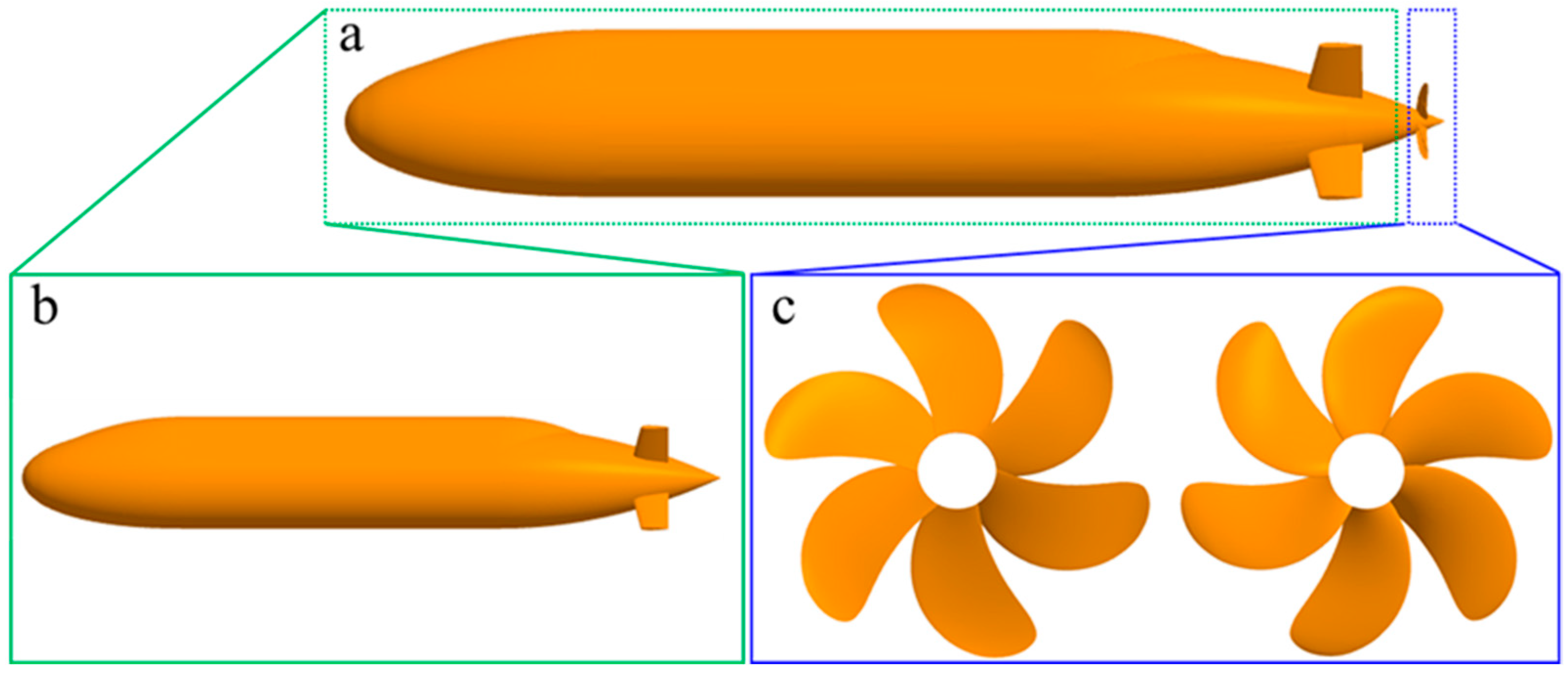
2. Research Model
3. Numerical Method
3.1. Control Equation and Turbulence Model
3.2. Free Surface Treatment
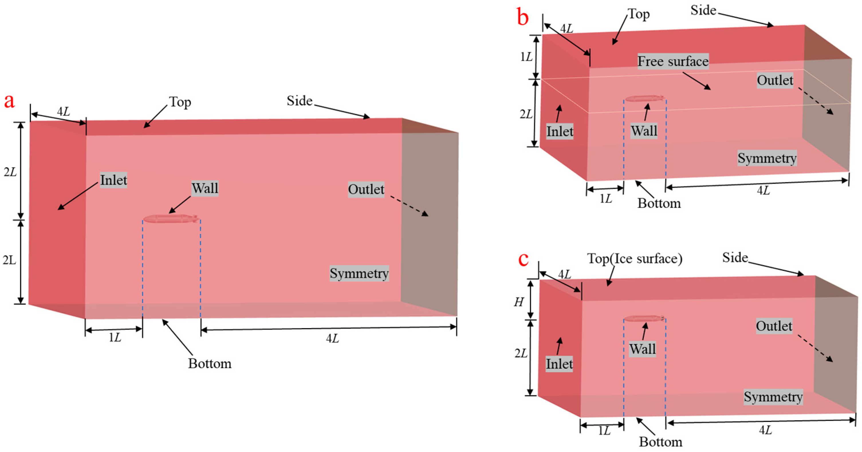
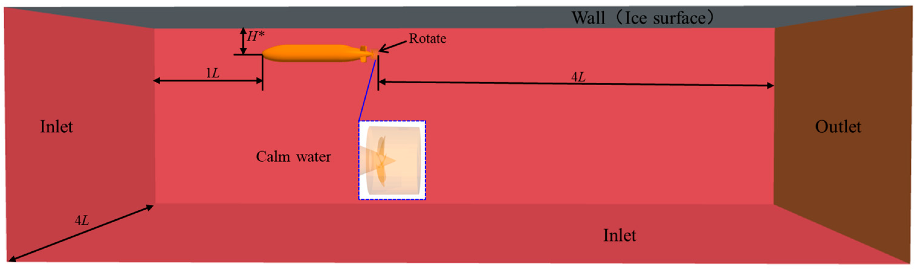
3.3. Computational Domain and Boundary Conditions
3.4. Time Step and Time Scale
3.5. Grid Convergence Analysis and Results Verification
4. Comparative Analysis with or Without Appendages
5. Calculation of Operating Conditions and Analysis of the Results (Without a Propeller)
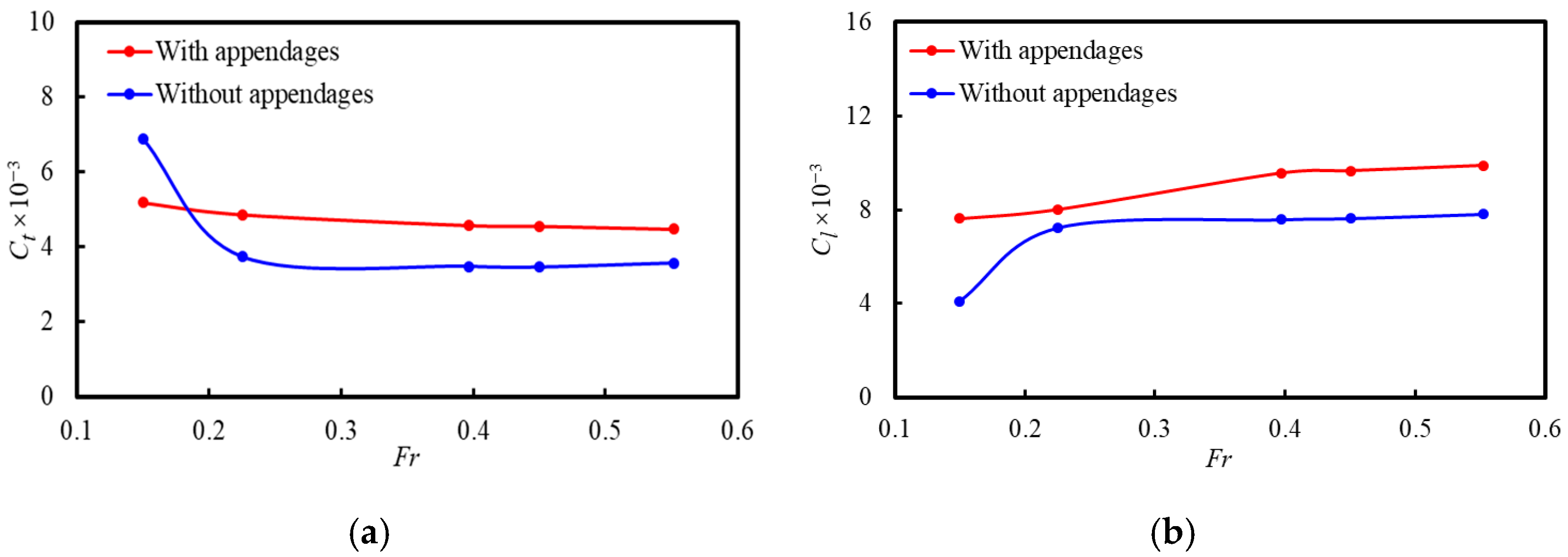
5.1. Resistance Coefficient Results and Analysis
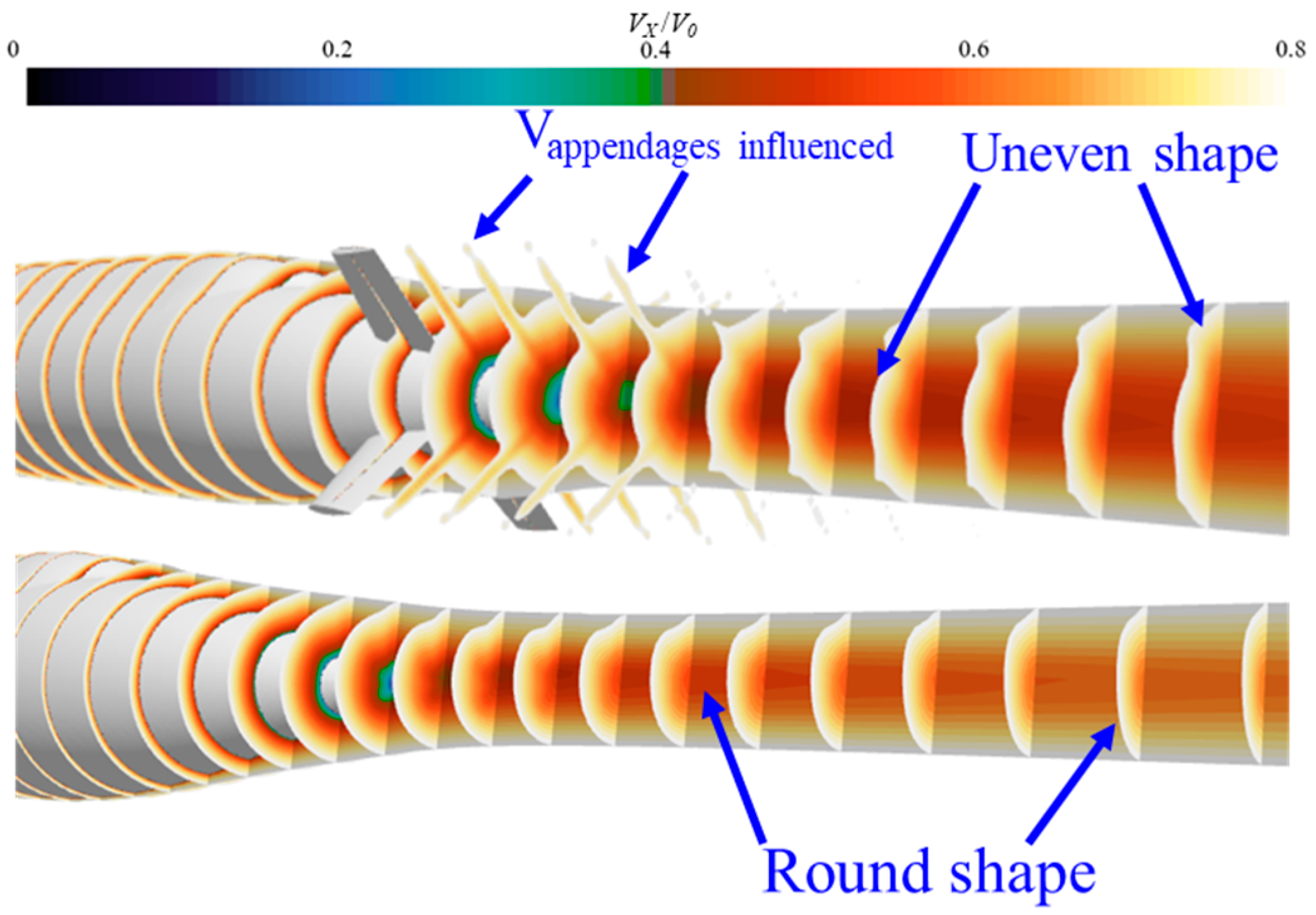
5.2. Velocity Field Analysis
5.3. Pressure Field
6. Comparison of Different Operating Conditions in Self-Propulsion
6.1. Model of Self-Propulsion Condition
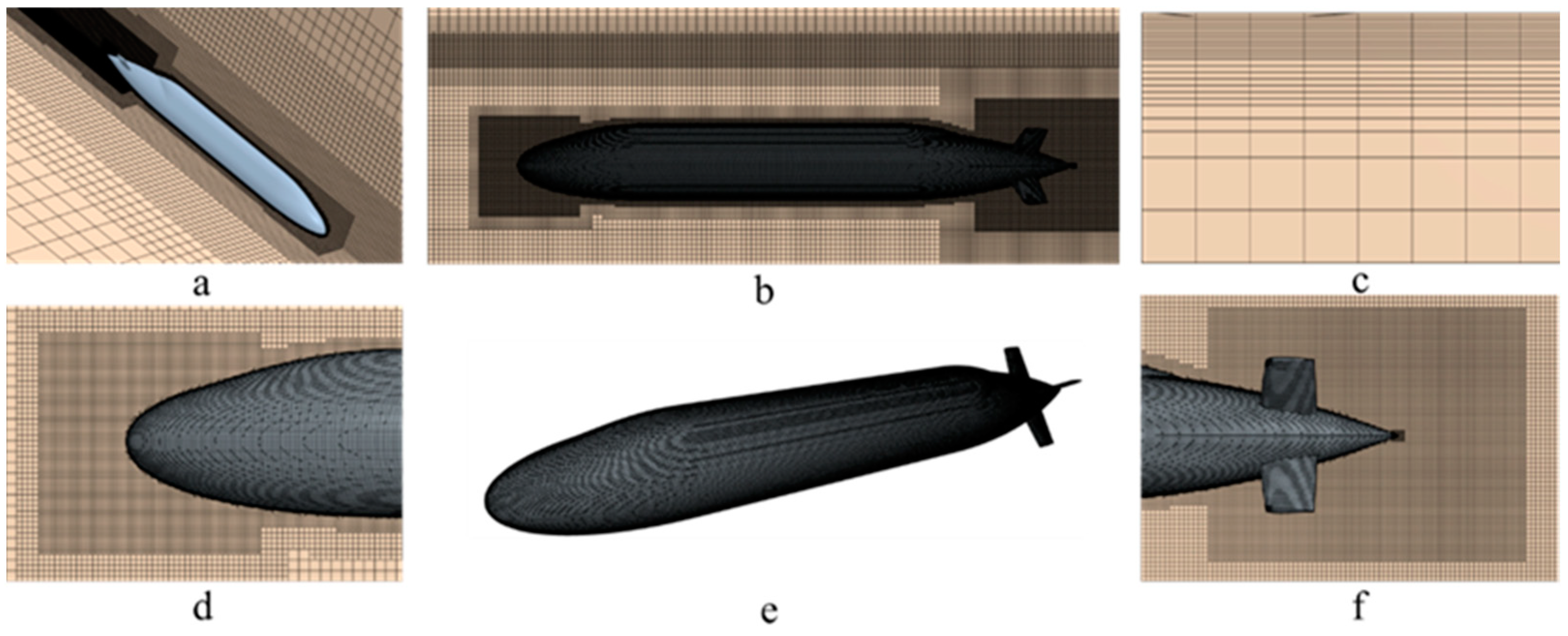
6.2. Computational Domains and Meshing at Self-Propulsion Condition
6.3. Meshing Sensitivity Study Under Self-Propulsion Condition
7. Calculations Conditions and Result Analysis Under Self-Propulsion Condition
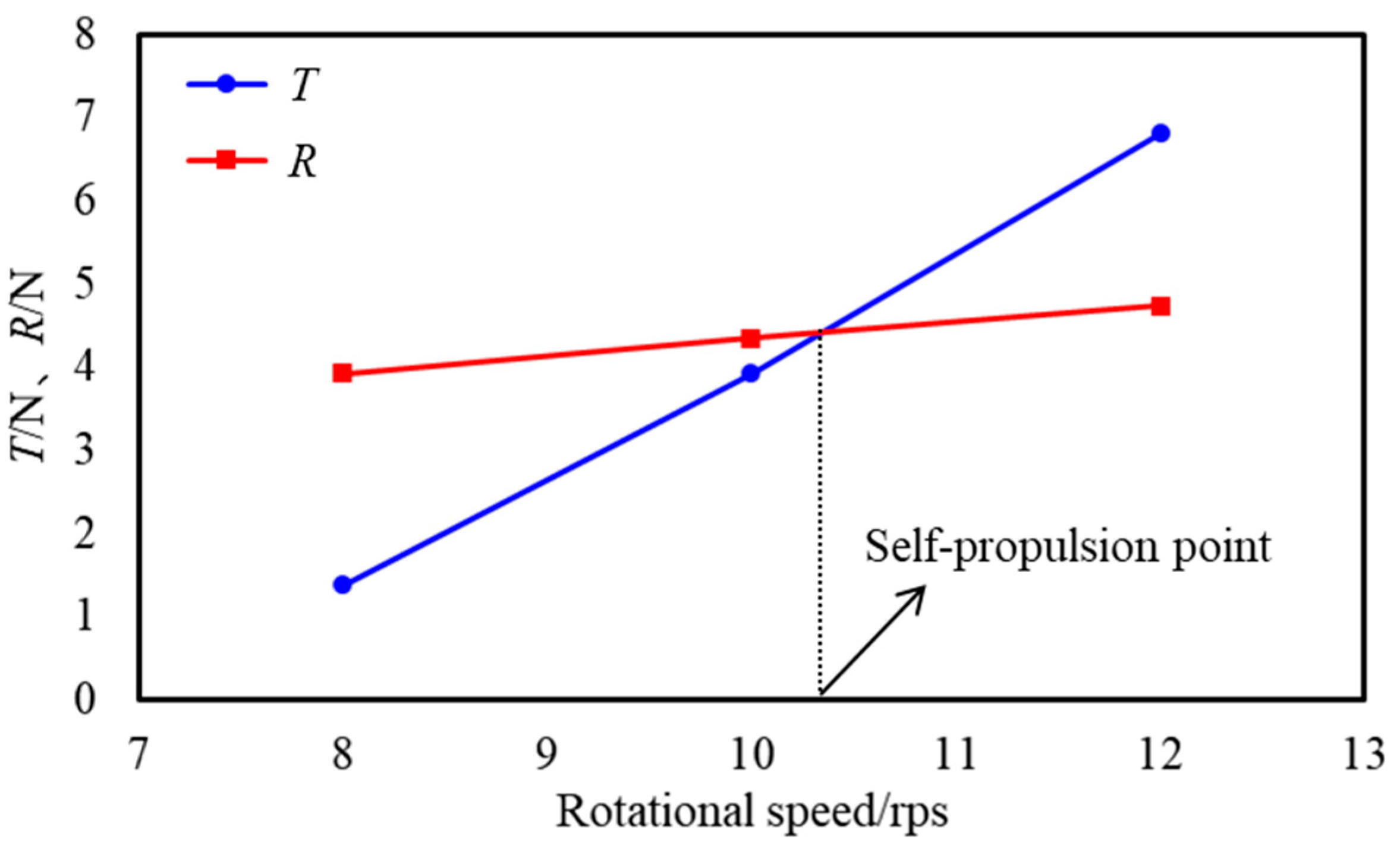
7.1. Rotational Speed at Self-Propulsion Point Under Different Self-Propulsion Conditions
7.2. Velocity Field Under Different Self-Propulsion Conditions
7.3. Pressure Field Under Different Self-Propulsion Conditions
8. Conclusions
- (1)
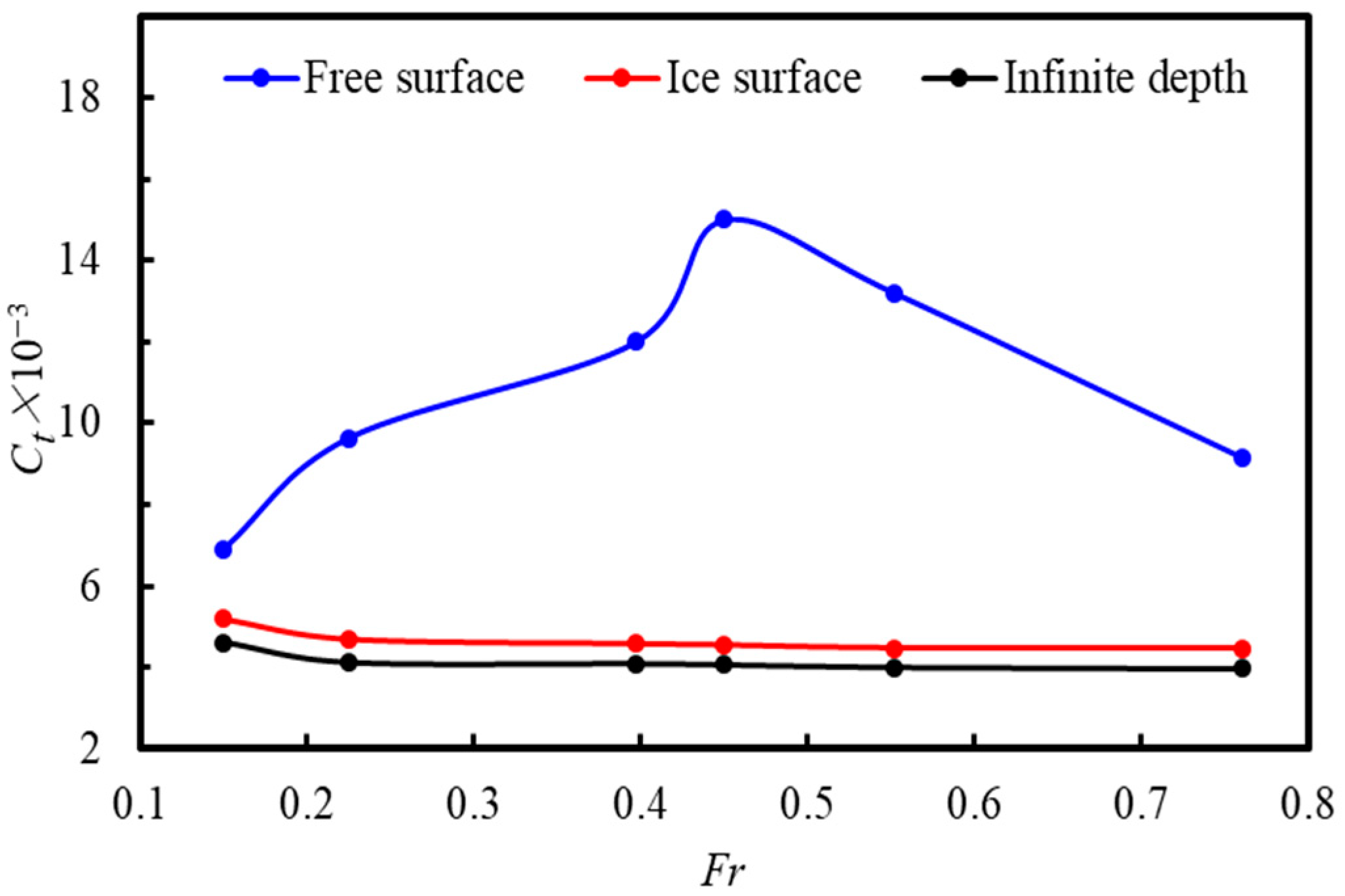
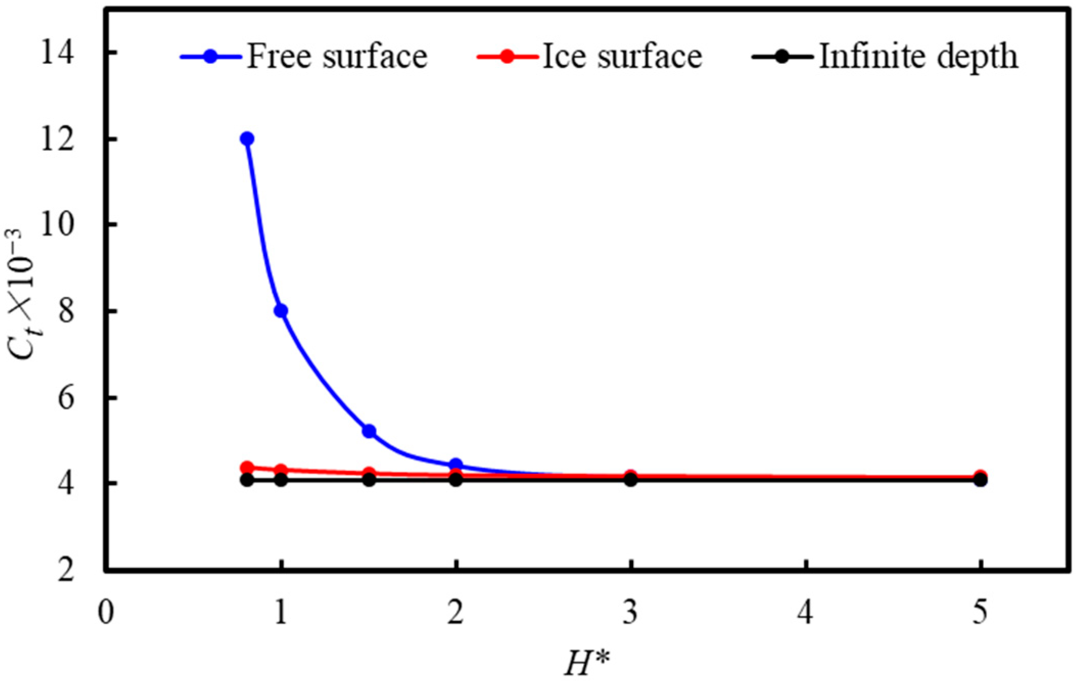
- During navigation near the free surface, the resistance coefficient of the vehicle is significantly greater than that observed during navigation at infinite depth and near the ice surface due to the influence of the free surface. The resistance coefficient decreases as the distance from the ice surface and the free surface increases. When the navigation depth exceeds 2D, the influence of the ice surface on the BB2 vehicle can be disregarded. Additionally, when H ≥ 3D, the influence of the free surface on the BB2 vehicle can also be ignored.
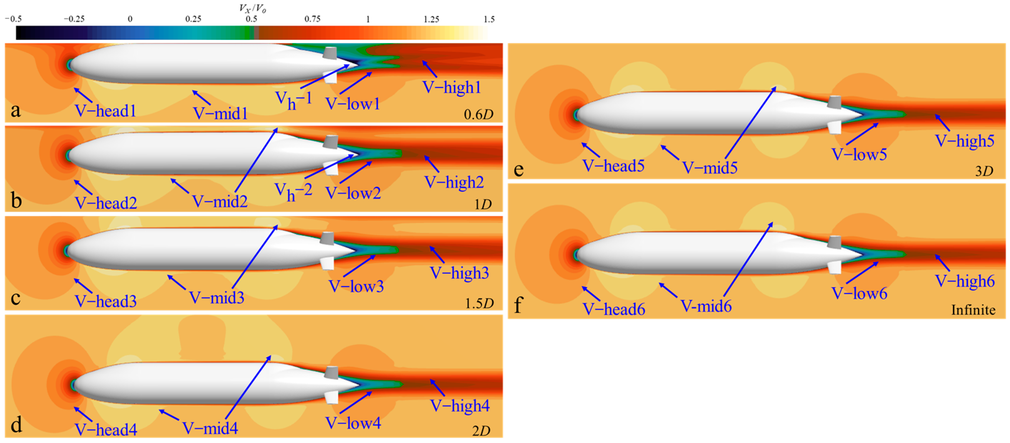
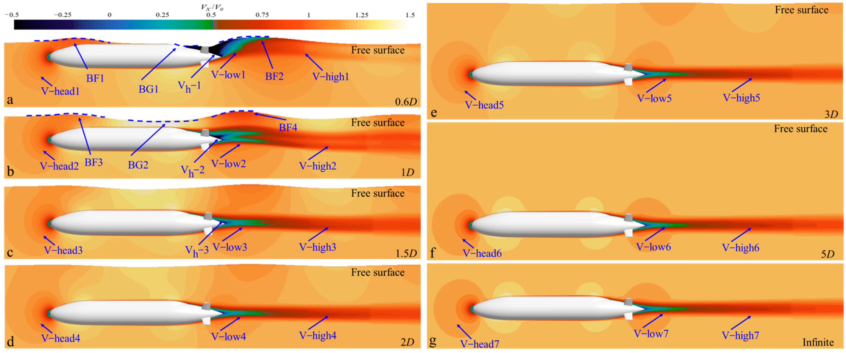
- (2)
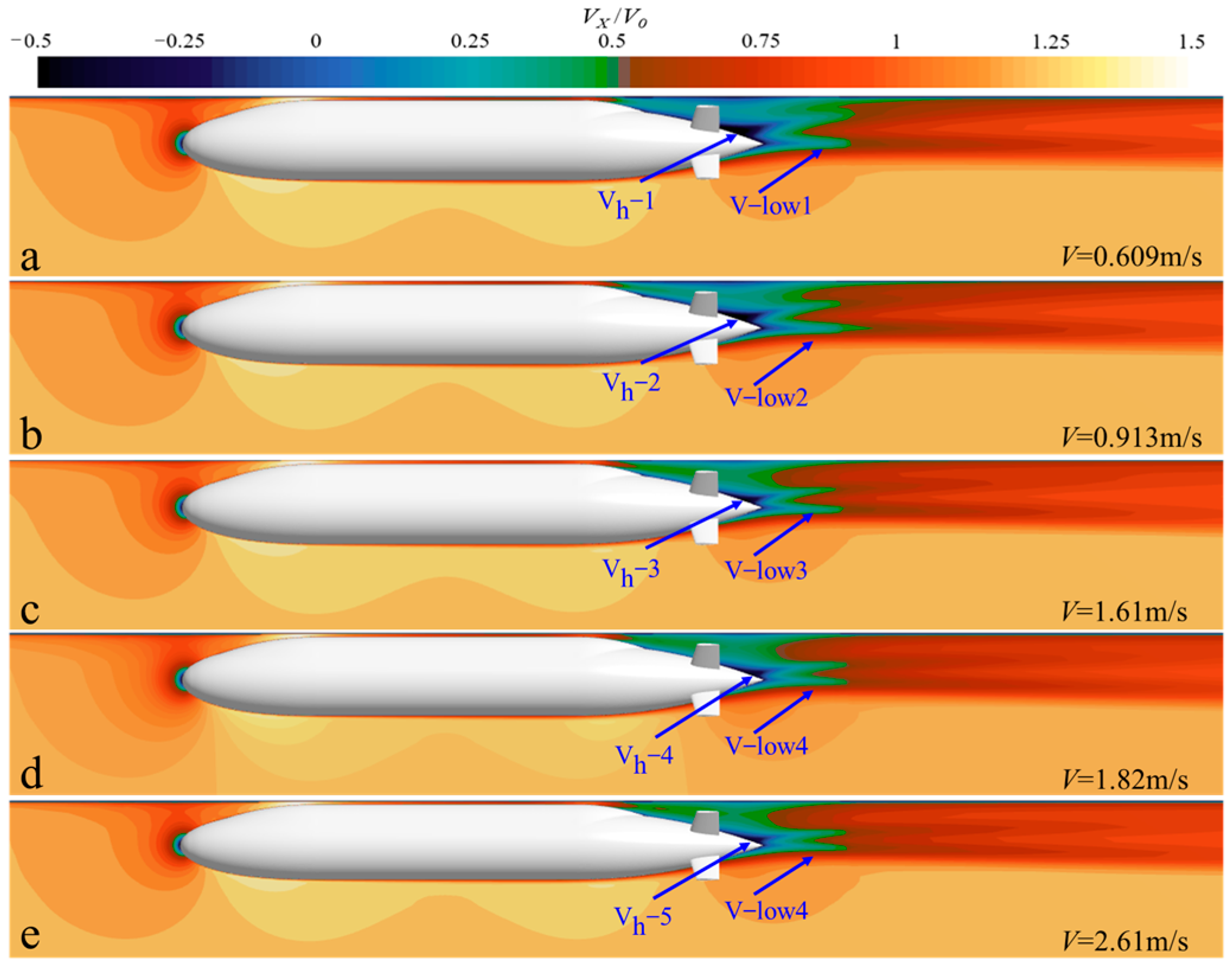
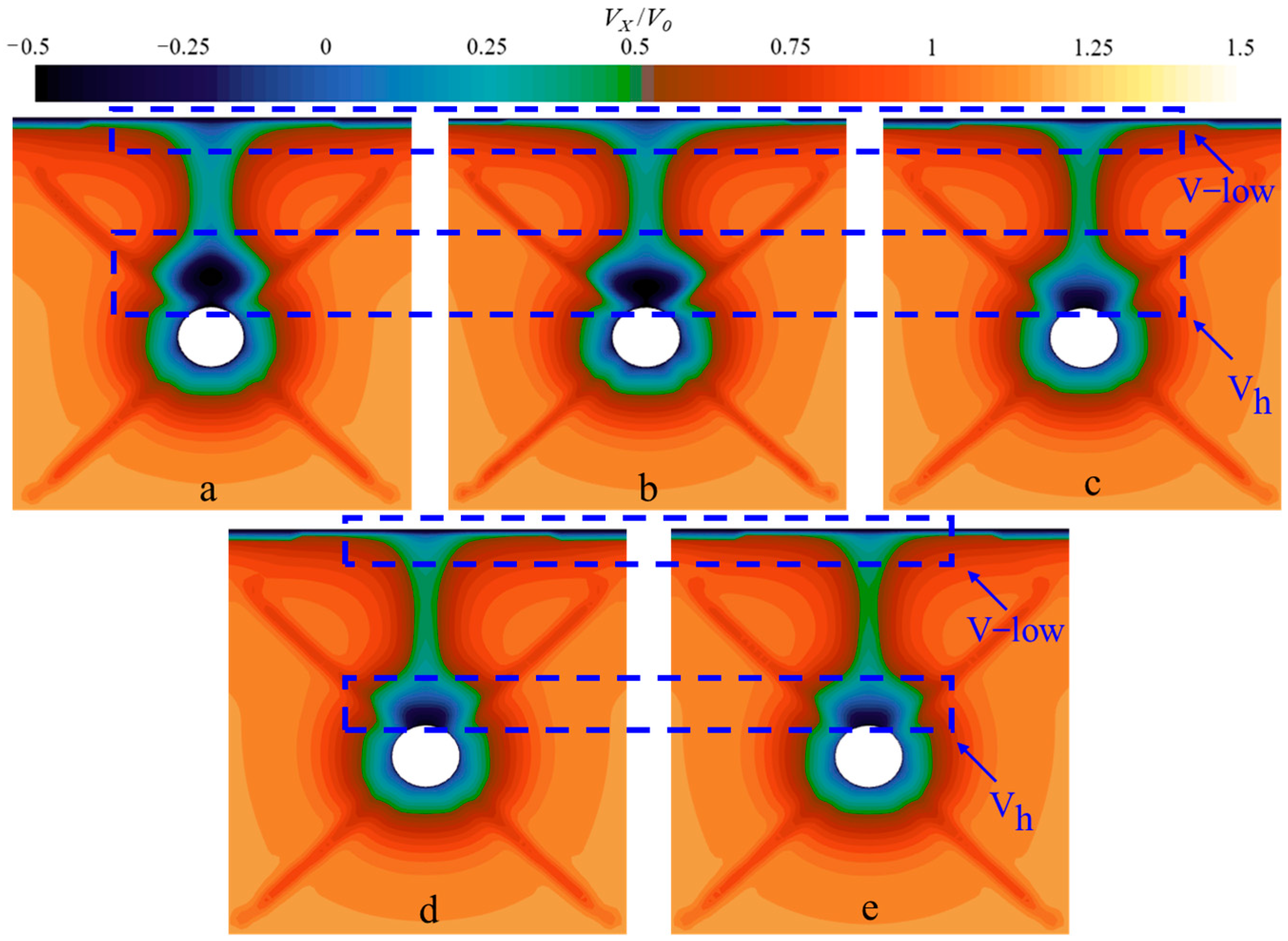
- Regardless of navigation near the continuous ice layer or near the free surface, the velocity field distribution of BB2 remains consistently asymmetric. During navigation near the ice surface, the ice surface has a significant adsorption effect on the wakefield of BB2. As the velocity increases, the adsorption effect gradually weakens. When the navigation depth is greater than 2D, the influence of the ice surface on the velocity field of BB2 gradually weakens.
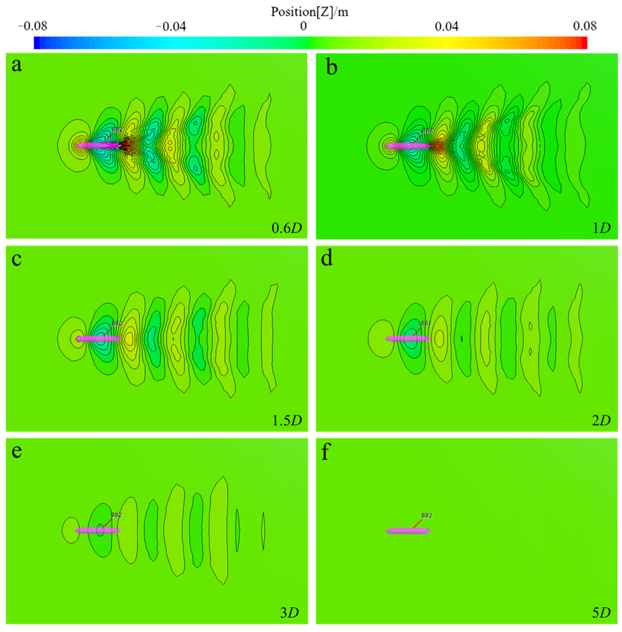
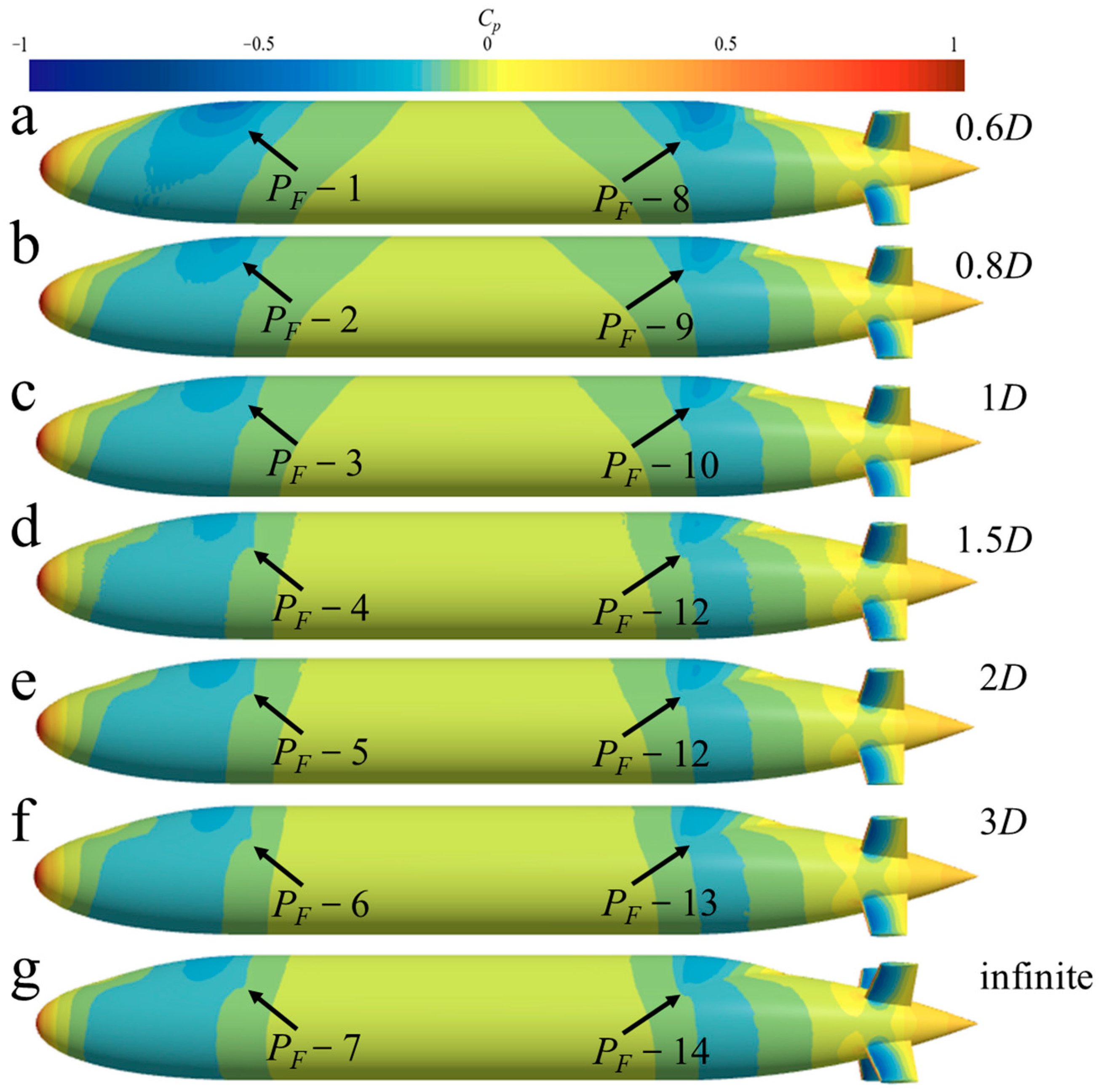
- (3)
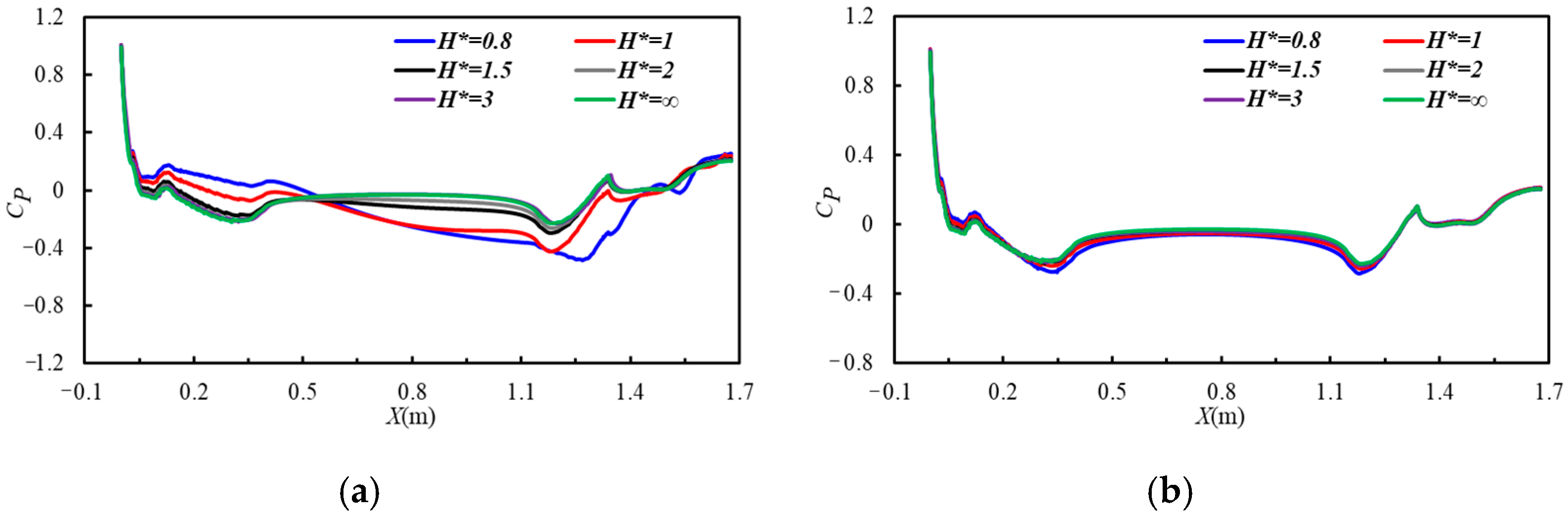
- During navigation near the continuous ice layer, negative pressure zones are observed at both the head and tail of BB2. The extent of these negative pressure zones gradually decreases with increasing distance from the ice surface. In contrast, when navigating near the free surface, the peaks and troughs of the free surface, there is a positive pressure zone at the tail. The influence of wave generation on the pressure field of BB2 is significantly greater than that of the ice surface.
- (4)
- During self-propulsion, when the diving depth H = 1D, due to the energy dissipation caused by wave generation at the free surface results in a significantly higher rotational speed at the self-propulsion point compared with that observed during self-propulsion near the ice surface. Consequently, the influence of the free surface on the vehicle’s velocity and pressure fields is marked greater than that of the ice surface.
Author Contributions
Funding
Institutional Review Board Statement
Informed Consent Statement
Data Availability Statement
Conflicts of Interest
References
- Li, Z.G.; Zhang, A.Q.; Yu, J.C. The Application Of Underwater Vehicles In Polar Expedition. Chin. J. Polar Res. 2004, 16, 135–144. [Google Scholar]
- Kukulya, A.; Plueddemann, A.; Austin, T.; Stokey, R.; Purcell, M.; Allen, B.; Littlefield, R.; Freitag, L.; Koski, P.; Gallimore, E. Under-ice operations with a REMUS-100 AUV in the Arctic. In Proceedings of the IEEE/OES Autonomous Underwater Vehicles, Monterey, CA, USA, 1–3 September 2010. [Google Scholar]
- Mcphail, S.D.; Pebody, M. Autosub-1. A distributed approach to navigation and control of an autonomous underwater vehicle. In Proceedings of the Seventh International Conference on Electronic Engineering in Oceanography, 1997, ‘Technology Transfer from Research to Industry’, Southampton, UK, 23–25 June 1997. [Google Scholar]
- Song, D.; Liu, H. Present Status and Key Technology of Autonomous Underwater Vehicle for Investigation in Polar Region. Mar. Electr. Electron. Eng. 2020, 40, 4. [Google Scholar]
- Li, Y.P.; Li, S.; Zhang, A.Q. Research status of autonomous/remotely controlled underwater vehicles. J. Eng. Stud. 2016, 8, 217–222. [Google Scholar]
- He, J.F. Briefing on China’s 36th Antarctic Scientific Expedition. Chin. J. Polar Res. 2020, 32, 3. [Google Scholar]
- Zhao, N. China’s 36th Antarctic Expedition (4) Underwater robots help Antarctic scientific expeditions. Sci. Explor. 2020, 9, 26–27. [Google Scholar]
- Tolliver, J.V. Studies on Submarine Control for Periscope Depth Operations. In Thesis Collect; PN Book: Stansted, UK, 1997. [Google Scholar]
- Sahin, I.; Crane, J.W.; Watson, K.P. Application of a panel method to hydrodynamics of underwater vehicles. Ocean Eng. 1997, 24, 501–512. [Google Scholar] [CrossRef]
- Jagadeesh, P.; Murali, K.; Idichandy, V.G. Experimental investigation of hydrodynamic force coefficients over AUV hull form. Ocean Eng. 2009, 36, 113–118. [Google Scholar] [CrossRef]
- Jagadeesh, P.; Murali, K. Rans Predictions of Free Surface Effects on Axisymmetric Underwater Body. Eng. Appl. Comput. Fluid Mech. 2010, 4, 301–313. [Google Scholar] [CrossRef]
- Shariati, S.K.; Mousavizadegan, S.H. The effect of appendages on the hydrodynamic characteristics of an underwater vehicle near the free surface. Appl. Ocean Res. 2017, 67, 31–43. [Google Scholar] [CrossRef]
- Wang, L.; Bi, Y.; Zhou, G.L.; Xiang, G.; Zhou, Y.P. Numerical study on submarine’s hydrodynamic performance for near-surface conditions. Ship Sci. Technol. 2021, 043, 83–88. [Google Scholar]
- Bai, T.; Xu, J.; Wang, G.D.; Yu, K.; Hu, X.H. Analysis of resistance and flow field of submarine sailing near the ice surface. Chin. J. Ship Res. 2021, 16, 13. [Google Scholar]
- Luo, W.; Jiang, D.; Wu, T.; Liu, M.; Li, Y. Numerical simulation of the hydrodynamic characteristics of unmanned underwater vehicles near ice surface. Ocean Eng. 2022, 253, 111304. [Google Scholar] [CrossRef]
- Wang, H.; Fang, E.; Hong, L. Numerical analysis of underwater hydrodynamic characteristics of submarine bare hull model. J. Harbin Eng. Univ. 2024, 1, 1–9. [Google Scholar]
- Liu, G.; Hao, Z.; Bie, H.; Wang, Y.; Ren, W.; Hua, Z. Control mechanism of a vortex control baffle for the horseshoe vortex around the sail of a DARPA SUBOFF model. Ocean Eng. 2023, 275, 114166. [Google Scholar] [CrossRef]
- Hao, Y.; Ding, J.; Bian, C.; Zhao, P.; Xia, L.; Wang, X.; Liu, H. Deep graph learning for the fast prediction of the wake field of DARPA SUBOFF. Ocean Eng. 2024, 309, 118353. [Google Scholar] [CrossRef]
- Liefvendahl, M.; Troëng, C. Computation of cycle-to-cycle variation in blade load for a submarine propeller using LES. In Proceedings of the Proc Second International Symposium on Marine Propulsors, Hamburg, Germany, June 2011. [Google Scholar]
- Chase, N.; Carrica, P. CFD simulations of a submarine propeller and application to self-propulsion of a submarine. Ocean Eng. 2013, 60, 68–80. [Google Scholar] [CrossRef]
- Sezen, S.; Dogrul, A.; Delen, C.; Bal, S. Investigation of self-propulsion of DARPA Suboff by RANS method. Ocean Eng. 2018, 150, 258–271. [Google Scholar] [CrossRef]
- Zhang, N.; Zhang, S.-l. Numerical simulation of hull/propeller interaction of submarine in submergence and near surface conditions. J. Hydrodyn. 2014, 26, 50–56. [Google Scholar] [CrossRef]
- Özden, Y.A.; Özden, M.C.; Demir, E.; Kurdoglu, S. Experimental and numerical investigation of DARPA Suboff submarine propelled with INSEAN E1619 propeller for self-propulsion. J. Ship Res. 2019, 63, 235–250. [Google Scholar] [CrossRef]
- Wang, L.; Martin, J.E.; Felli, M.; Carrica, P.M. Experiments and CFD for the propeller wake of a generic submarine operating near the surface. Ocean Eng. 2020, 206, 107304. [Google Scholar] [CrossRef]
- Li, P.; Wang, C.; Han, Y.; Qi, Y.F.; Wang, S.M. The Study Aboout The Impact of the Free-Surface on the Performance of the Propeller Attached at the Stern of a Submarine. Chin. J. Theor. Appl. Mech. 2021, 53, 2501–2514. [Google Scholar]
- Lungu, A. A DES-based study of the flow around the self-propelled DARPA Suboff working in deep immersion and beneath the free-surface. Ocean Eng. 2022, 244, 110358. [Google Scholar] [CrossRef]
- Kim, D.-J.; Kwon, C.-S.; Lee, Y.-Y.; Kim, Y.-G.; Yun, K. Practical 6-DoF manoeuvring simulation of a BB2 submarine near the free surface. Ocean Eng. 2024, 312, 119334. [Google Scholar] [CrossRef]
- Ding, Y.; Li, X.-R.; Yan, Y.; Wang, W.-Q. Investigation of the self-propulsion performance of a submarine with a pump-jet propulsor in a surface wave–current coupling environment. Ocean Eng. 2024, 312, 119306. [Google Scholar] [CrossRef]
- Hirt, C.W.; Nichols, B.D. Volume of fluid (VOF) method for the dynamics of free boundaries. J. Comput. Phys. 1981, 39, 201–225. [Google Scholar] [CrossRef]
- Luo, W. Study on the Resistance and Wake Field Characteristics of Ship-Ice-Water Coupling in Ice Floe Areas. Ph.D Thesis, Harbin Engineering University, Harbin, China, 2019. [Google Scholar]
- Carrica, P.M.; Kim, Y.; Martin, J.E. Near-surface self propulsion of a generic submarine in calm water and waves. Ocean Eng. 2019, 183, 87–105. [Google Scholar] [CrossRef]
- Roy, C.J.; Heintzelman, C.; Roberts, S.J. Estimation of Numerical Error for 3D Inviscid Flows on Cartesian Grids. In Proceedings of the 45th AIAA Aerospace Sciences Meeting and Exhibit, Reno, NV, USA, 8–11 January 2007. [Google Scholar]
- Huang, S.; Liu, W.; Luo, W.; Wang, K. Numerical simulation of the motion of a large scale unmanned surface vessel in high sea state waves. J. Mar. Sci. Eng. 2021, 9, 982. [Google Scholar] [CrossRef]
- Dawson, E. An Investigation into the Effects of Submergence Depth, Speed and Hull Length-to-Diameter Ratio on the Near Surface Operation of Conventional Submarines. Master’s Thesis, University of Tasmania, Hobart, Australia, 2014. [Google Scholar]
- McHale, M.; Friedman, J.; Karian, J. Standard for Verification and Validation in Computational Fluid Dynamics and Heat Transfer; The American Society of Mechanical Engineers: New York, NY, USA, 2009; Volume 20, p. 100. [Google Scholar]
- Wei, M.; Chiew, Y.-M. Impingement of propeller jet on a vertical quay wall. Ocean Eng. 2019, 183, 73–86. [Google Scholar] [CrossRef]
- Roache, P.J. Quantification of Uncertainty in Computational Fluid Dynamics. Ann. Rev. Fluid Mech. 1997, 29, 123–160. [Google Scholar] [CrossRef]
- Pan, Y.-C.; Zhang, H.-X.; Zhou, Q.-D. Numerical simulation of unsteady propeller force for a submarine in straight ahead sailing and steady diving maneuver. Int. J. Nav. Archit. Ocean Eng. 2019, 11, 899–913. [Google Scholar] [CrossRef]


| Overall Length [m] | 1.679 |
| Diameter (D) [m] | 0.23 |
| Truncated Model Length (LM) [m] | 1.607 |
| Star of parallel midbody aft of leading edge [m] | 0.383 |
| End of parallel midbody aft of leading edge [m] | 1.149 |
| Wetted Surface Area (S) [m2] | 1.041 |
| Hull Prismatic Coefficient | 0.785 |
| Boundary Name | Boundary Conditions | ||
|---|---|---|---|
| Infinite Depth | Near Free Surface | Near Ice Surface | |
| Inlet/Bottom Side/Symmetry | Velocity inlet | Velocity inlet, velocity based on flat VOF wave along the X-direction | Velocity inlet |
| Outlet | Pressure outlet | Pressure outlet, based on flat VOF wave hydrodynamic pressure | Pressure outlet |
| Wall | No slip, impenetrable and fixed wall | No slip, impenetrable and fixed wall | No slip, impenetrable and fixed wall |
| Top | Velocity inlet | Velocity inlet, velocity based on flat VOF wave along the X-direction | No slip, impenetrable wall with X-direction velocity (ice surface) |
| Velocity [m/s] | Basic Size | Number of Meshes | Experimental Results [N] | Numerical Results [N] | Error |
|---|---|---|---|---|---|
| 1.61 | 0.05 | coarse | 4.516 | 4.612 | 2.12% |
| 0.03 | medium | 4.516 | 4.57 | 1.20% | |
| 0.01 | fine | 4.516 | 4.515 | −0.02% |
| Variables | RG | PG | UG |
|---|---|---|---|
| Resistance | 1.31 | 1.12 | 0.0038 |
| H | Fr | With Appendages | Without Appendages | ||
|---|---|---|---|---|---|
| Ct × 10−3 | Cl × 10−3 | Ct × 10−3 | Cl × 10−3 | ||
| 0.6 D | 0.15 | 5.19 | 7.63 | 6.9 | 4.1 |
| 0.2250 | 4.87 | 8.02 | 3.74 | 7.23 | |
| 0.397 | 4.58 | 9.56 | 3.48 | 7.58 | |
| 0.45 | 4.56 | 9.66 | 3.46 | 7.63 | |
| 0.552 | 4.48 | 9.88 | 3.57 | 7.81 | |
| Items | Geometric Parameter | Unit |
|---|---|---|
| blades | 6 | piece |
| Dpro | 0.118 | m |
| Dhub/Dpro | 0.2 | - |
| AE/AO | 0.80 | - |
| P0.7Rpro | 0.997 | - |
| Velocity [m/s] | Number of Meshes | R [N] | T [N] |
|---|---|---|---|
| 1.61 | coarse-1 | 3.97 | 4.40 |
| medium-1 | 3.92 | 4.34 | |
| fine-1 | 3.88 | 4.30 |
| Variables | RG | PG | UG |
|---|---|---|---|
| R | 0.8 | 2 | 0.0017 |
| T | 0.67 | 2 | 0.0013 |
| H | Conditions | Rotational Speed [rps] | T [N] | R [N] | Rotational Speed at Self-Propulsion Point [rps] |
|---|---|---|---|---|---|
| 0.6D | Free surface | 13 | 8.83 | 10.5 | 13.94 |
| 15 | 12.96 | 11.07 | |||
| 17 | 17.93 | 11.85 | |||
| Ice surface | 8 | 1.46 | 4.45 | 10.77 | |
| 10 | 3.89 | 4.9 | |||
| 12 | 7.02 | 5.42 | |||
| 1D | Free surface | 9 | 2.76 | 6.32 | 11.95 |
| 11 | 5.47 | 6.89 | |||
| 13 | 8.94 | 7.36 | |||
| Ice surface | 8 | 1.37 | 4.11 | 10.6 | |
| 10 | 3.79 | 4.57 | |||
| 12 | 6.89 | 5.07 | |||
| 2D | Free surface | 8 | 2.2 | 4.93 | 10.46 |
| 10 | 4.6 | 5.21 | |||
| 12 | 7.72 | 5.7 | |||
| Ice surface | 8 | 1.379 | 3.92 | 10.450 | |
| 10 | 3.82 | 4.38 | |||
| 12 | 6.88 | 4.95 | |||
| ∞ | Infinite | 8 | 1.379 | 3.92 | 10.459 |
Disclaimer/Publisher’s Note: The statements, opinions and data contained in all publications are solely those of the individual author(s) and contributor(s) and not of MDPI and/or the editor(s). MDPI and/or the editor(s) disclaim responsibility for any injury to people or property resulting from any ideas, methods, instructions or products referred to in the content. |
© 2024 by the authors. Licensee MDPI, Basel, Switzerland. This article is an open access article distributed under the terms and conditions of the Creative Commons Attribution (CC BY) license (https://creativecommons.org/licenses/by/4.0/).
Share and Cite
Xu, P.; Chen, J.; Guo, Y.; Luo, W. Comparative Study on Hydrodynamic Characteristics of Under-Water Vehicles Near Free Surface and Near Ice Surface. J. Mar. Sci. Eng. 2024, 12, 2131. https://doi.org/10.3390/jmse12122131
Xu P, Chen J, Guo Y, Luo W. Comparative Study on Hydrodynamic Characteristics of Under-Water Vehicles Near Free Surface and Near Ice Surface. Journal of Marine Science and Engineering. 2024; 12(12):2131. https://doi.org/10.3390/jmse12122131
Chicago/Turabian StyleXu, Pei, Jixiang Chen, Yingchun Guo, and Wanzhen Luo. 2024. "Comparative Study on Hydrodynamic Characteristics of Under-Water Vehicles Near Free Surface and Near Ice Surface" Journal of Marine Science and Engineering 12, no. 12: 2131. https://doi.org/10.3390/jmse12122131
APA StyleXu, P., Chen, J., Guo, Y., & Luo, W. (2024). Comparative Study on Hydrodynamic Characteristics of Under-Water Vehicles Near Free Surface and Near Ice Surface. Journal of Marine Science and Engineering, 12(12), 2131. https://doi.org/10.3390/jmse12122131