1. Introduction
Unmanned surface vehicles (USVs), also known as Autonomous Surface Vessels (ASVs), are capable of autonomous navigation and operations. They are often deployed in complex and harsh oceanic environments, which necessitate robust autonomous navigation capabilities. This autonomous navigation serves as the foundation for subsequent tasks such as collision avoidance, automatic docking, target tracking, and formation control. Among these capabilities, autonomous trajectory tracking is a critical aspect that highlights the USV’s navigational proficiency. When navigating dynamic ocean environments with significant wave and wind disturbances, USVs face time-varying external interferences and limitations due to their underactuated nature, leading to reduced navigational stability and increased difficulty in trajectory tracking. Over the years, researchers have relentlessly explored the trajectory tracking control mechanisms of USVs under wave and wind conditions.
Do K. D. [
1] investigated the trajectory tracking control of USVs in the presence of wind and wave disturbances using the Serret–Frenet frame. An adaptive robust trajectory tracking controller for underactuated USVs was developed by designing nonlinear observers for the lateral velocity and yaw rate based on nonlinear backstepping and the Lyapunov stability theory [
2].
Sun [
3] designed an exponentially stable trajectory tracking controller for USVs based on the dynamic surface control theory. Aguiar A. P. [
4] researched trajectory tracking control for USVs using switching control techniques, while Fahimi F. [
5] proposed a robust sliding mode trajectory tracking control method. Harmouche M. [
6] addressed the lack of speed measurement feedback in the trajectory tracking of USVs by proposing a control method based on observer technology and backstepping. Katayama H. [
7] introduced a straight-line trajectory tracking control method for underactuated vessels with semi-global uniform asymptotic stability, utilizing nonlinear sampled-data control theory, state feedback, output feedback control techniques, and observer technology [
8,
9]. However, the aforementioned methods, including optimal control, feedback linearization, and backstepping, require precise modeling to achieve high control accuracy [
10]. The motion model of a USV is affected by variables such as speed and load, making precise modeling challenging. Moreover, disturbances from wind, waves, and currents during navigation complicate the path-following control of USVs. Therefore, in real oceanic environments, control algorithms based on deterministic models or those with non-adaptive control parameters often fail to achieve the desired control performance.
The PID control algorithm remains dominant in ship autopilot systems because of its simplicity and reliability. However, when USVs experience substantial time-varying disturbances, the effectiveness of fixed-parameter PID algorithms is not satisfactory. Researchers have sought to enhance the effectiveness through improving the adaptability of PID parameters [
11]. Most efforts are focused on combining PID with other theories such as fuzzy control and neural networks to achieve the adaptive tuning of PID parameters.
Adaptive PID controllers adjust PID parameters dynamically during the process of tracking a desired heading, significantly enhancing the algorithm’s dynamic response. However, due to model uncertainties and external disturbances, a discrepancy between the estimated and actual system outputs often exists. Hu Zhiqiang [
12] proposed an online self-optimizing PID heading control algorithm, which facilitates the online adjustment of control parameters and exhibits robust performance and interference resistance.
Genetic algorithms (GAs), known for their stable global optimization capabilities, are frequently used for parameter tuning in various USV path controllers. Liu [
13] has demonstrated the use of GA for the online tuning of PID parameters to implement adaptive PID control. However, these controllers face challenges such as prolonged parameter optimization times, which can impact the real-time applicability on actual vessels. Designing crossover and mutation operators within the optimization process can shorten the optimization time and enhance the algorithm’s real-time performance [
14].
Fuzzy logic control translates expert knowledge into fuzzy rules; it can effectively address the impacts of model uncertainties and random disturbances on USV path-following control. In practical applications, fuzzy logic is often used for the parameter tuning of PID controllers and sliding mode controllers due to its rapid response and real-time performance [
15,
16]. Liu [
15] has established fuzzy rules according to path point errors, heading errors, and error differentials to improve control smoothness. However, the accuracy of fuzzy controllers mainly depends on the complexity of the fuzzy rules, which is generally constructed based on expert knowledge and dynamic models, so complex rules may lead to computational challenges [
17].
Peng Yan [
18] researched the challenges faced by USV systems, such as large inertia, long time delays, nonlinearity, difficulty in precise modeling, and susceptibility to external disturbances like waves. The study revealed that traditional PID control often fails to achieve satisfactory trajectory tracking performance. Consequently, a PID cascade controller based on generalized predictive control (GPC-PID) was designed to separately control the heading and steering motions of USVs, providing enhanced resistance to external disturbances. Additionally, radial basis function (RBF) neural networks can approximate model uncertainties and external disturbances affecting PID parameters, thus improving the robustness and interference resistance of the controller. RBF neural networks are frequently employed to model the impact of internal and external disturbances on PID parameters.
Reinforcement Learning (RL) has been extensively applied in control systems [
19]. Its capability to operate without precise mathematical models and its self-learning abilities make it particularly effective in addressing challenges related to model uncertainties and unknown disturbances in USV trajectory tracking control [
20,
21]. Neural networks were utilized within sliding mode controllers to tune controller parameters, with RL employed to evaluate the tuning efficacy [
22]. This approach enabled the self-learning of neural network parameters, addressing the low model accuracy requirement of sliding mode control while mitigating its chattering issue.
Sun [
3] explored trajectory tracking control for underactuated USVs under unknown disturbances using neural network control technologies. Another study [
23] employed Q-learning for PID parameter tuning, demonstrating that this controller can effectively resist external disturbances and facilitate the motion control of mobile robots through experiments. Bertaska [
24] developed a multi-mode switching controller using Q-learning, which intelligently switches controllers based on the environment and the operational state of the USV, enhancing control performance across different conditions.
Magalhaes [
25] proposed a RL control method based on Q-learning that mimics fish swimming motions to control the fins and tail of an unmanned underwater vehicle (UUV) for trajectory tracking. Bian [
26] employed neural network controllers for ship trajectory tracking control; however, such learning methods require the pre-acquisition of reliable ship navigation sample data. Deep Q Networks (DQNs), which incorporate experience replay and fixed Q-targets, significantly enhance the stability and expressiveness of complex RL problems [
27]. However, DQNs remain constrained to discrete action or state spaces based on Q-learning, making them challenging to apply to the continuous control problem of USV motion under dynamic wave conditions, where low control precision can lead to chattering.
Wu [
28] modeled the trajectory tracking problem as a Markov Decision Process (MDP) based on the maneuvering characteristics and control requirements of ships. The DDPG algorithm was used as the controller, and offline learning methods were applied for controller training. Simulation tests showed promising results, although the simulation environment lacked environmental disturbances. Woo [
29] introduced a trajectory tracking controller based on Deep Reinforcement Learning (DRL), allowing USVs to learn navigation experiences during voyages. In repetitive trajectory tracking simulations, the control strategy was trained to enable adaptive interaction with the environment, achieving trajectory following. However, this method directly employed DRL as the control strategy rather than adaptive parameter matching, which lacks the mature performance of classical control algorithms. Additionally, it did not leverage the dynamic performance of USVs within the controller, but treated it as a black box, which demands high-quality training data. Without comprehensive training data, the control performance may not meet expectations.
The analysis above highlights several key issues in the current trajectory tracking control methods for USVs: Firstly, many existing algorithms fail to consider the impact of time-varying environmental disturbances. Secondly, when employing machine learning algorithms for training USV motion controllers, acquiring sample data poses significant challenges, and the quality of these training samples greatly influences the performance of machine learning-based controllers. Thirdly, when using RL algorithms such as Q-learning for controller training, these approaches typically use a black box method to compensate for time-varying and difficult-to-quantify environmental disturbances. However, the motion and control models established by these methods are based on discrete mathematical models with low precision. Fourthly, directly using RL as a controller, rather than for adaptive parameter tuning, fails to leverage the superior performance of classical control algorithms and relies entirely on black box processes, which preclude the utilization of USV dynamics within the controller.
To address these challenges, this paper proposes a trajectory tracking control algorithm for USVs that calculates PID control parameters based on an improved Deep Deterministic Policy Gradient (DDPG) algorithm. By integrating RL algorithms with classical control theory, this approach aims to enhance the adaptability of USV motion controllers. The subsequent sections of this paper are organized as follows:
Section 2 introduces the maneuvering motion model and parameters for USVs, the guidance law for path tracking, and the PID control algorithm employed.
Section 3 provides a detailed explanation of the proposed method for calculating PID parameters based on the improved DDPG algorithm and outlines the state, action, and reward settings for training the RL model.
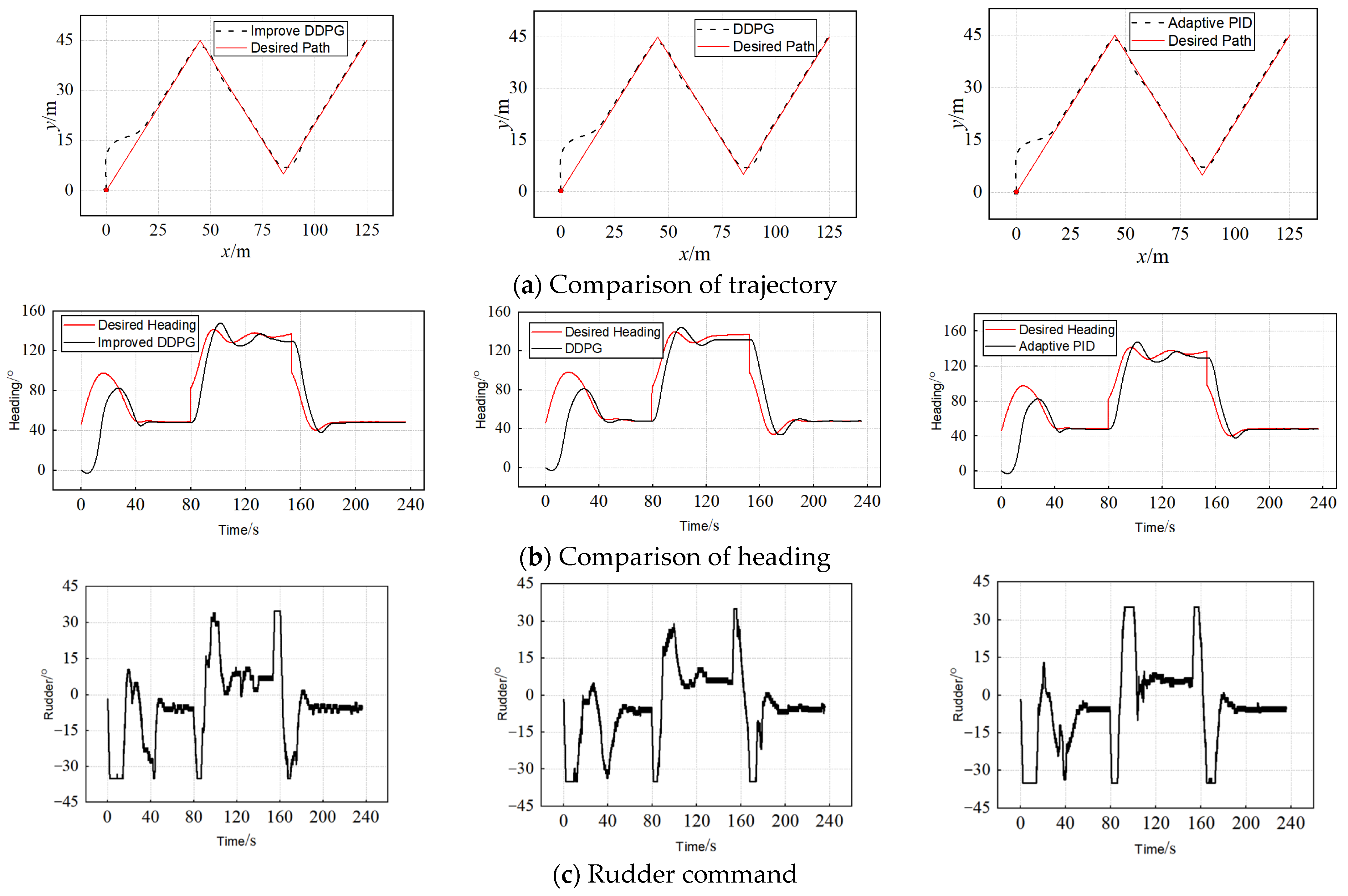
Section 4 presents the simulation results of various algorithms, demonstrating the superiority of the algorithm proposed in this study. In
Section 5, maneuvering experiment in wave conditions was conducted in a marine tank using the proposed algorithm, proving its feasibility and effectiveness.
3. PID Parameter Calculating Model Based on an Improved DDPG Algorithm
3.1. Algorithm Description
The tracking control process of USVs is a time-sequential decision-making problem characterized by MDPs. Thus, a USV can be regarded as an agent, with its motion control expressed in the form of . Herein, the details are as follows:
- a.
is the state transition matrix and refers to the probability of transitioning to the next state after applying action in the current state .
- b.
, the state set encompasses all states and exhibits the Markov property; that is, future states depend only on the current state and are independent of past states.
- c.
, the action set, comprises all possible actions that the agent can select. State transitions depend not only on the environment but also on the agent’s ability to guide state transitions by selecting different actions.
- d.
, the reward function, maps states and actions to rewards, reflecting preferences for different states.
Executing actions transitions the system from an initial state to a terminal state, forming a trajectory
, represented as
where
is the initial state,
is the terminal state, and
is the action chosen at time step i.
The aim is to maximize the cumulative reward
along the trajectory, expressed as
where
is the terminal time,
is the reward at time
, and
is the discount factor, with values ranging between 0 and 1.
To maximize the cumulative reward
, the policy
must be continuously optimized. The policy
maps states
to actions
, and the agent chooses actions based on the observed state according to the policy. The strategy that maximizes the cumulative reward is called the optimal policy, denoted as
.
where
is the expectation,
is the trajectory
based on policy
.
The goal of RL is to find the optimal policy
.
denotes the optimal action value function, can be used to provide the best action, and can be recursively expressed based on the Bellman equation:
where
denotes the next state derived from the environment transition probability
, and
represents the subsequent action obtained from the policy
.
, the best actions, can be recursively expressed by the Bellman equation.
In policy-based methods, the policy is denoted as
, where
represents a set of parameters constituting the policy. The goal is to maximize the expected return
, and gradient ascent is employed to update the parameters
and optimize the policy.
where
is the policy gradient.
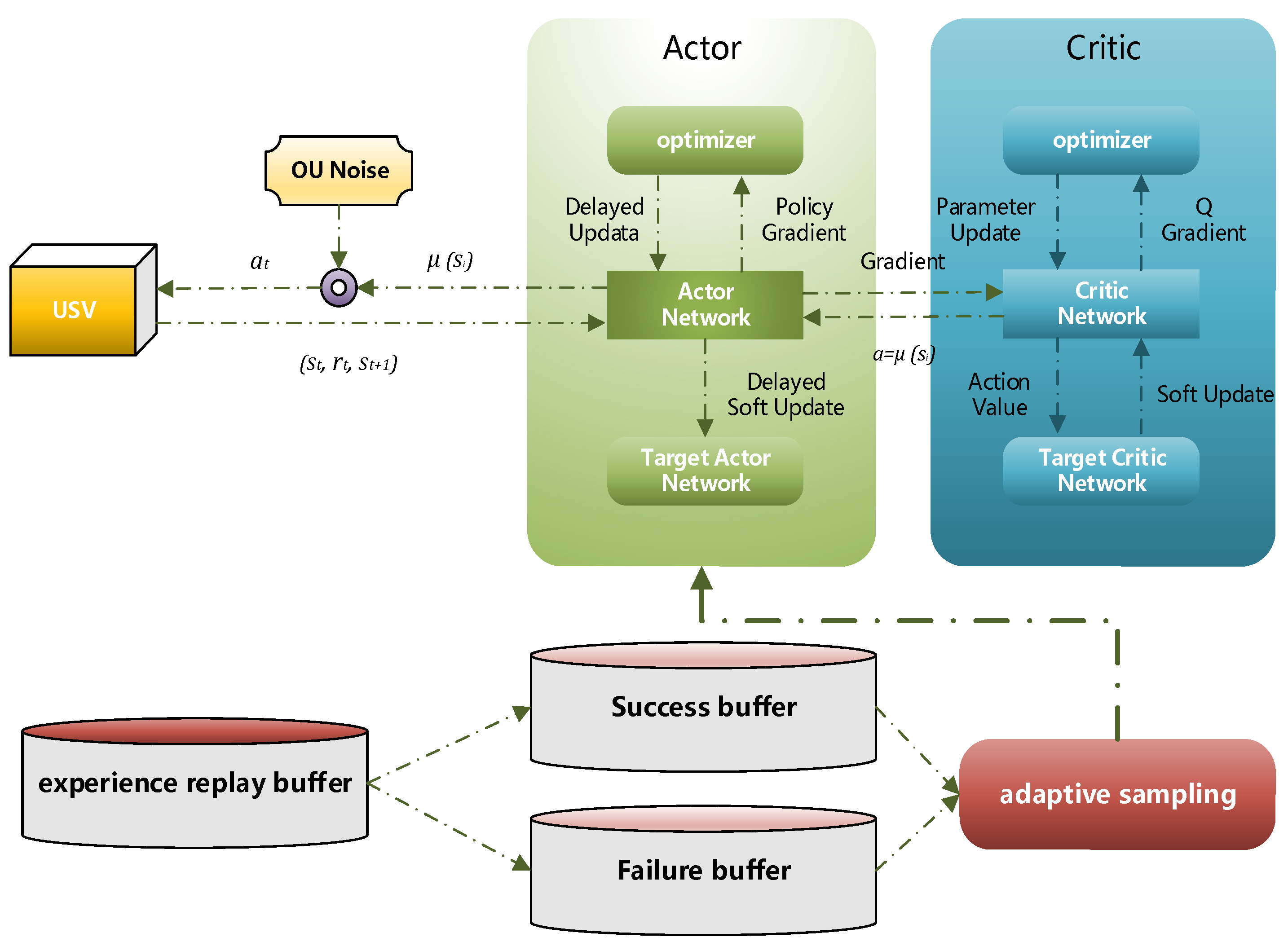
The improved DDPG algorithm in this study utilizes an Actor–Critic architecture, comprising four networks, detailed as follows:
- (1)
Current Actor Network
The input to the current Actor is the state space
, and the output is the action
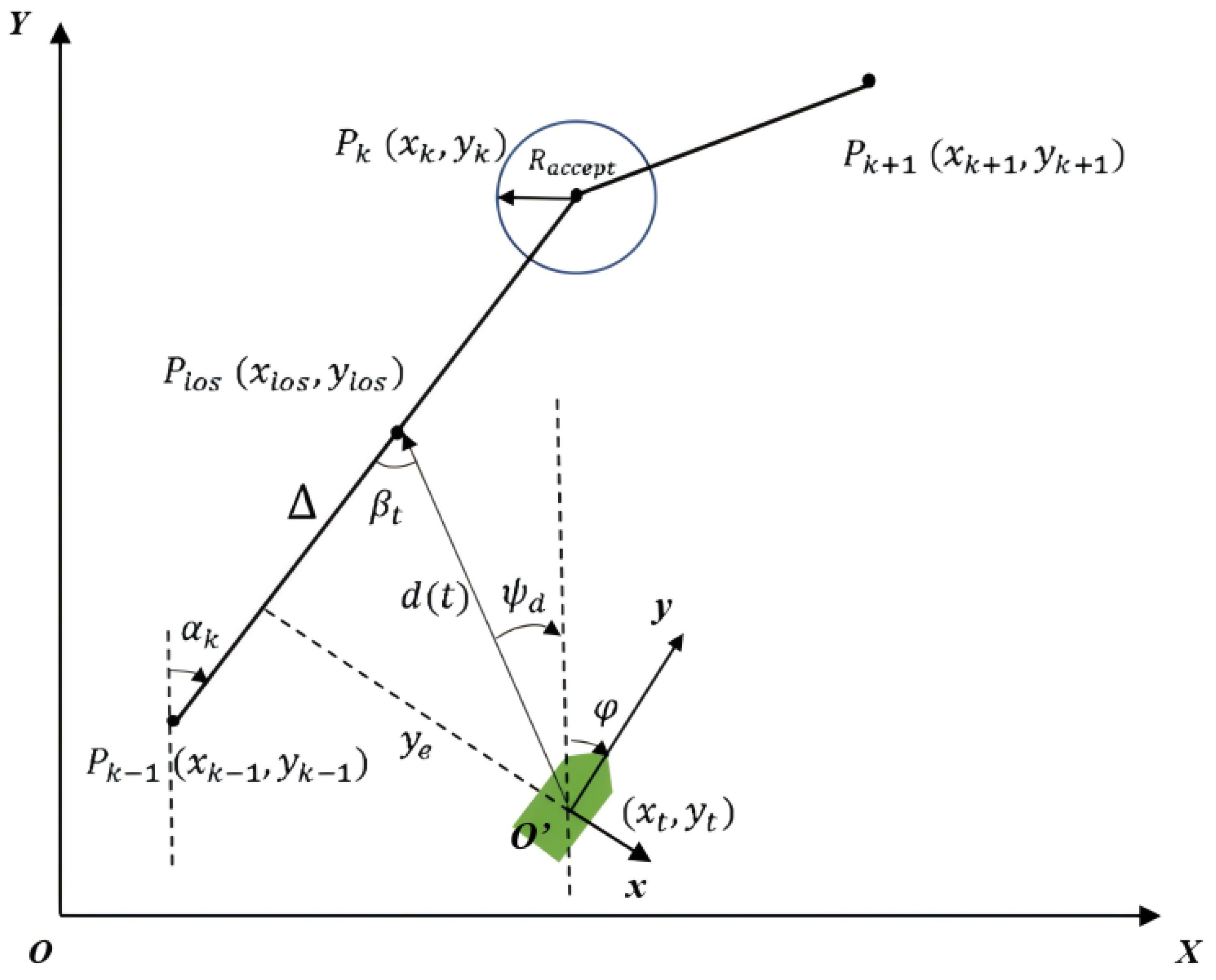
. In this study, the state space is defined as
where
and
are the longitudinal and lateral velocities,
is the yaw rate,
is the heading angle,
is the lateral deviation from the target trajectory,
is the rudder angle, and
is the inclination angle of the target trajectory. The action
is defined as
The objective of updating the Actor is to maximize the Q-value evaluated by the current Critic network. Thus, the gradient of the Actor is updated via backpropagation through the Critic’s gradient.
The Actor network architecture, as shown in
Figure 3, consists of an input layer, two hidden layers, and an output layer. The input layer has a dimension of 10, the two hidden layers contain 400 and 300 neurons, and the output layer has a dimension of 2. To extract features effectively, and also to prevent gradient saturation and vanishing problems, ReLU is used in the hidden layers and Tanh is used in the output layer.
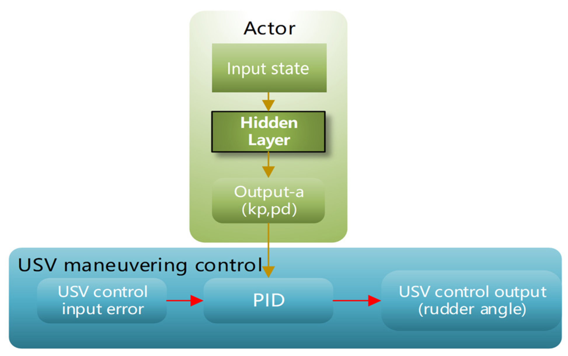
Figure 4 illustrated the relationship between the Actor network and USV motion controller. During training in the simulation system, the Actor outputs actions based on the input state through its neural network. These actions, representing PID control parameters, are utilized for USV motion control. The control deviation of the USV is used as input to obtain the USV control output variables, such as steering actions in heading control. Consequently, the USV executes steering actions, which are resolved through the rudder force model in the simulation environment, resulting in the USV’s subsequent motion posture.
- (2)
Target Actor Network
The Target Actor network generates target actions
, which are fed into the Target Critic network. The structure of the Target Actor mirror that of the current Actor network. Its weights are obtained via soft updates from the current Actor’s weights using Polyak averaging:
where
represents the target network parameters,
is the current network parameters, and
is a small coefficient. The arrow symbol used here is used to update
. This slow update process maintains the stability and relative independence of the target network, facilitating smoother changes that enhance algorithm stability and convergence.
- (3)
Current Critic network
The current Critic network evaluates the value of action
in state
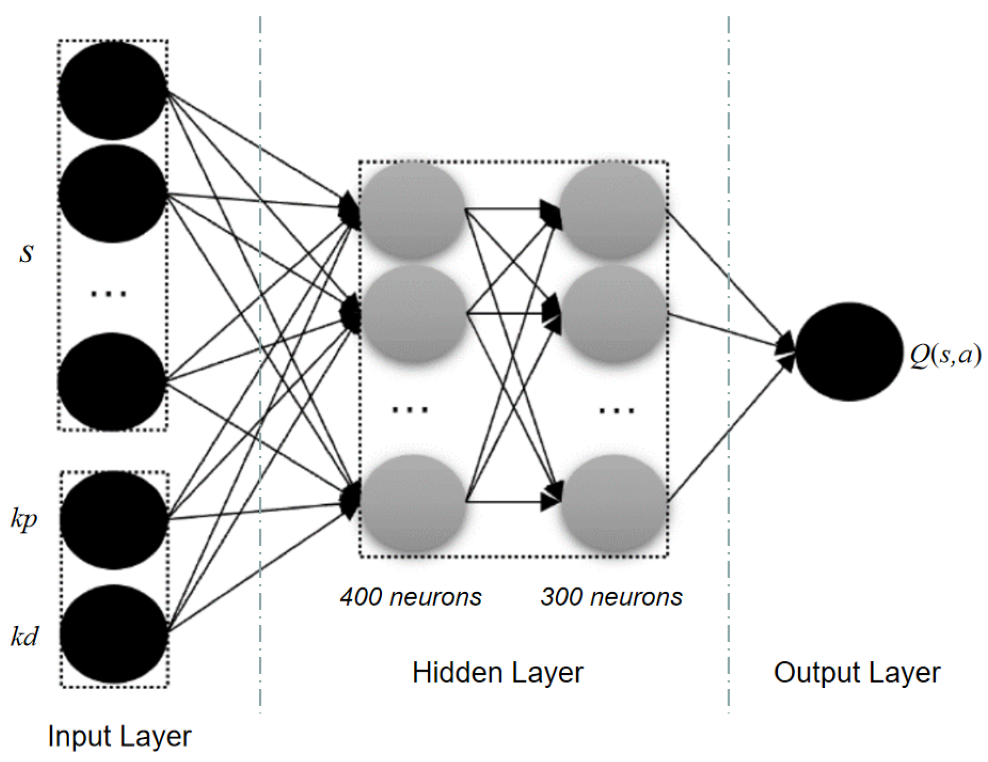
. Training the current Critic network requires target values, which are computed using the Target Critic and Target Actor networks. The current Critic is a feedforward neural network; its structure is depicted in
Figure 5. The input is a concatenation of the environmental state
and action
, outputting the state-action value
. The hidden layers contain 400 and 300 neurons, and the output layer dimension is 1, representing the state-action value.
- (4)
Target Value Network (Target Critic)
The Target Critic network calculates the target Q-value and, combined with the actual reward , computes the TD error, which is used to update the weights of the current Critic network. The structure of the Target Critic network mirrors that of the current Critic but is used for target updates. Its weights are also obtained through soft updates from the current Critic’s weights. The input consists of the environmental state and action , and the output is the state-action value .
3.2. Ornstein–Uhlenbeck (OU) Noise
OU noise is a time-correlated stochastic process initially used to describe Brownian motion in physics. In RL, it is employed to generate smooth and orderly noise sequences that aid in exploring the action space. The mathematical expression for the OU process is
where
is the value of the noise at time t,
is the parameter controlling the speed of noise regression to the mean,
is the long-term mean of the noise,
is the intensity of noise fluctuations, and
is the standard Brownian motion.
At each time step, the noise is updated according to the following OU process:
where
is a normal distribution with mean 0 and variance 1. When executing the strategy, the generated OU noise is added to the actions derived from the deterministic strategy.
3.3. Binary Experience Pool Based on Adaptive Batching
To address the slow training speed of the DDPG algorithm, the experience pool is divided into a success experience pool and a failure experience pool. To eliminate correlations between data, an adaptive batch size function is designed, where
experiences are sampled from each of the success and failure pools. New experience is gained from the environment (including the current state, action taken, reward received, next state, and termination status), and it is added to the buffer. During each current network training session, a random batch of experiences is sampled from the buffer, effectively breaking the temporal correlation between experiences and ensuring that training data are more independently and identically distributed.
In this context, represents the number of training iterations, and denotes the total number of training iterations set.
The overall algorithmic process is as follows:
- 1.
The Actor generates a set of actions, to which OU noise is added.
- 2.
The agent obtains the next state based on the current action and inputs it into the reward function. The data from is categorized into the successful experience pool or the failed experience pool based on success or failure.
- 3.
A sample of experiences is drawn from the experience pool, and both and are input into the Actor network, while are fed into the Critic network, where iterative updates are performed.
- 4.
The Target Actor network receives and ; inputs action and random noise into the agent, which interacts with the environment to obtain the next action ; and outputs it to the Target Critic network. The action values are then received to update the network.
- 5.
The Target Critic network receives
and
and calculates the Q-values. These values are then combined with the rewards to compute the labels used for iterative network updates. See
Figure 6.
3.4. Reward Definition and Analysis
Based on the maneuvering characteristics of USVs and the features of path tracking control, the reward function is defined as follows:
The reward function comprehensively considers both the lateral deviation and heading angle deviation in trajectory tracking, with the expectation that both deviations remain minimal. According to the reward setting, if the heading angle deviation is less than 0.1, the reward is 0. Conversely, if the heading angle deviation exceeds 0.1, a negative reward is generated, with the magnitude of the negative reward positively correlated with the consecutive heading angle deviations. This design aims to use RL to reduce the heading angle deviation. For lateral deviation, the requirement is to keep it within 1 m. Within this range, the lateral deviation reward is 0, but if it exceeds 1 m, a negative reward of −0.1 is applied, aiming to reduce lateral deviation through RL.
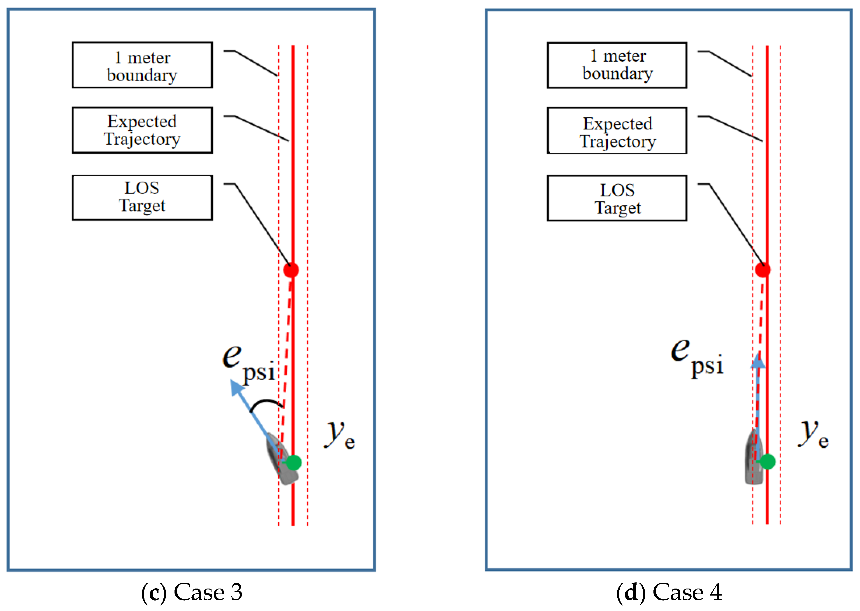
Below is an analysis of typical scenarios based on this reward setting (see
Figure 7):
- (a)
, : As illustrated in the scenario, both the lateral and heading angle deviations receive significant negative rewards (on the order of −0.1). During training, actions receiving nearly 0 rewards will be emphasized, guiding the USV to alter its heading angle toward the LOS target point and reduce lateral error. According to the reward setting, the priority between altering the motion direction toward the LOS target point and approaching the tracking trajectory to reduce lateral deviation is dynamically adjusted.
- (b)
, : In this scenario, the lateral deviation receives a significant negative reward (on the order of −0.1), while the negative reward for heading angle deviation is minor (close to 0). During training, actions with nearly 0 rewards are reinforced, guiding the USV to approach the tracking trajectory to reduce lateral error without excessively adjusting the heading angle, which could lead to increased lateral deviation and negative rewards for heading angle deviation. According to the reward setting, the priority between turning toward the LOS target point and approaching the tracking trajectory is dynamically adjusted.
- (c)
, : Here, the lateral deviation receives a minor negative reward (close to 0), while the heading angle deviation incurs a significant negative reward (on the order of −0.1). During training, actions yielding nearly 0 rewards are emphasized, guiding the USV to adjust its heading angle toward the LOS target to reduce the heading angle deviation. However, due to the inertia of USV motion and the narrow 1 m reward boundary for lateral deviation, if the heading angle deviation is substantial, the USV might overshoot the 1 m boundary during adjustment, resulting in oscillation around the tracking trajectory. To avoid this, the USV should not have excessive heading angle deviation when entering this scenario.
- (d)
, : In this case, both lateral and heading angle deviations receive minor negative rewards (close to 0). The USV’s trajectory tracking control tends to stabilize, meeting the tracking requirements and maintaining this condition despite wave disturbances. However, if the USV enters this scenario and maintains stability, there may exist a steady-state lateral error of less than 1 m. With 0 rewards for both lateral and heading angle deviations, this steady-state error might not be corrected. This issue can be addressed by dynamically changing the LOS target point, but this requires a longer training time.
5. Experimental Results and Analysis
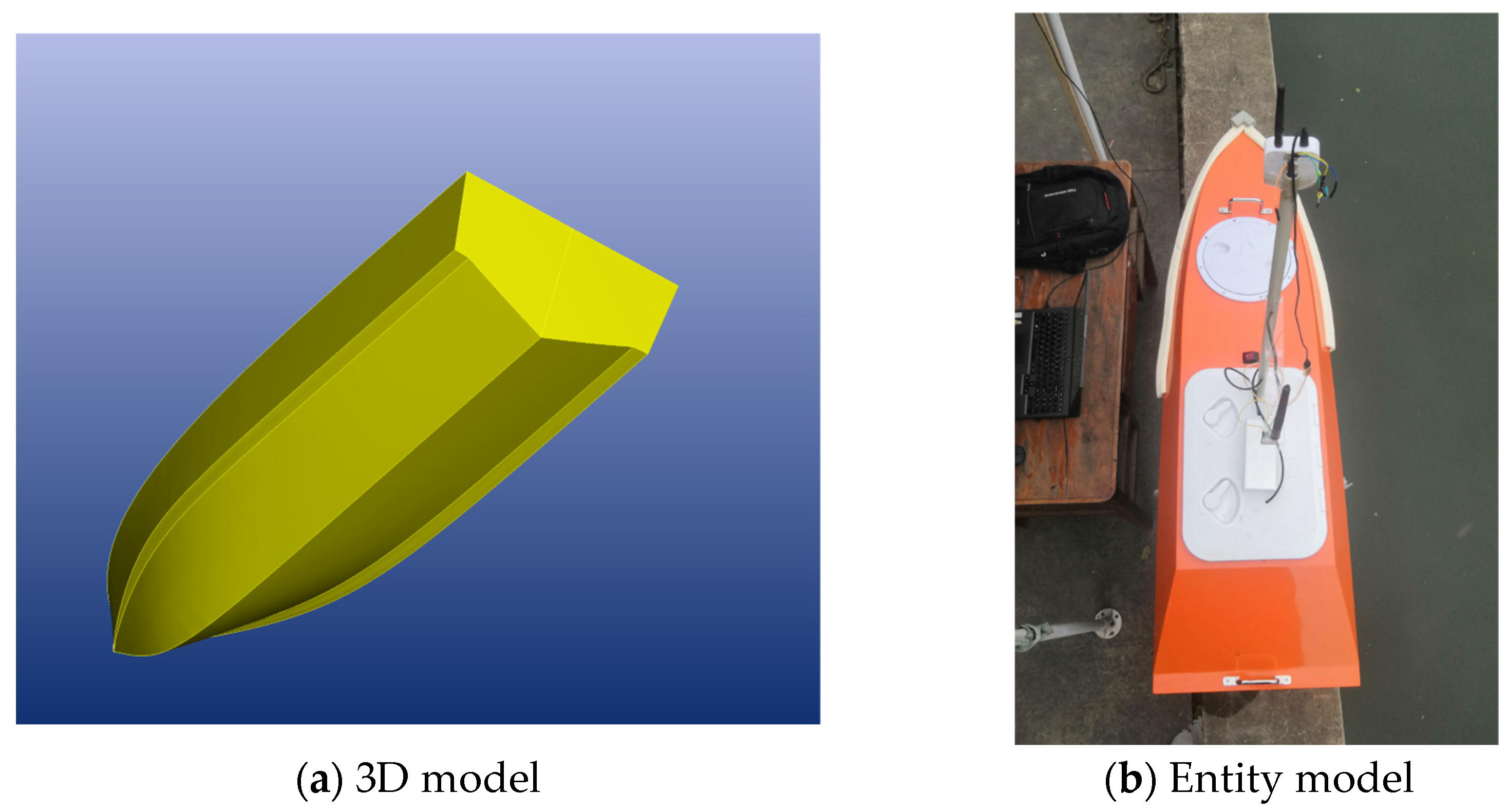
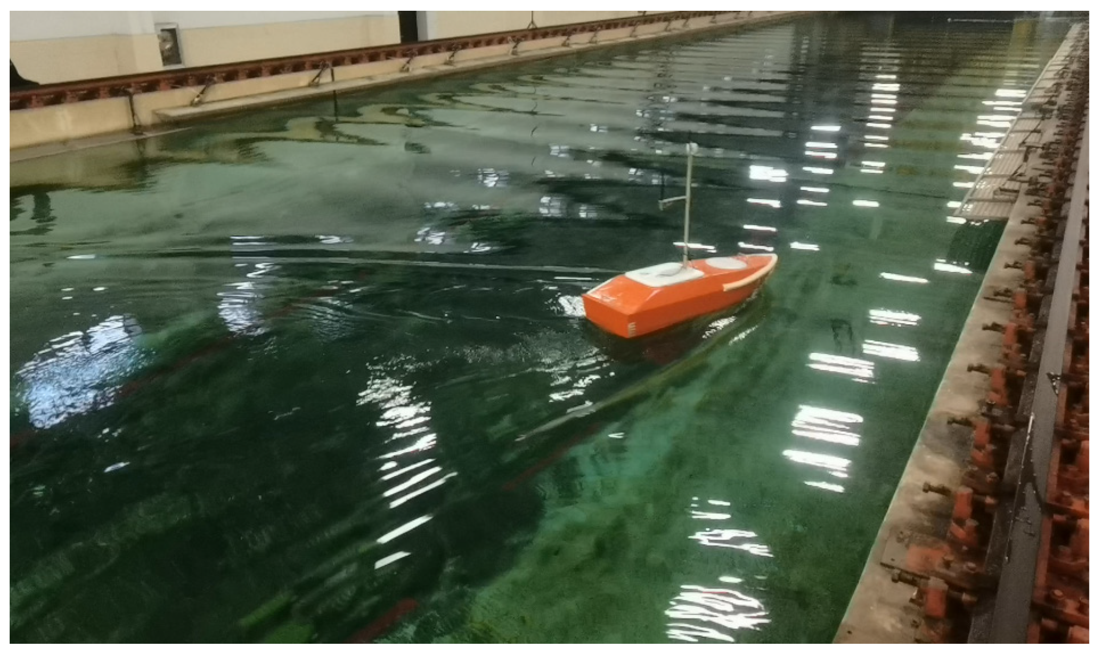
It is challenging to conduct curve tracking experiments due to the wave maker located in the ship towing tank, which has a limited width. Therefore, this study conducted Zigzag trajectory tracking control experiments under wave conditions only. The positioning equipment used was an indoor UWB system, and the USV was equipped with a gyroscope for heading, a servo motor for propeller adjustment, and a rudder servo for steering. The main control board was an STM32, facilitating wireless serial communication with the host computer. The host computer sent commands to the model ship, and the USV transmitted real-time sensor data back to the host for display. Simultaneously, the host computer performed control calculations based on the collected data, utilizing the proposed improved DDPG algorithm for calculating PID parameters.
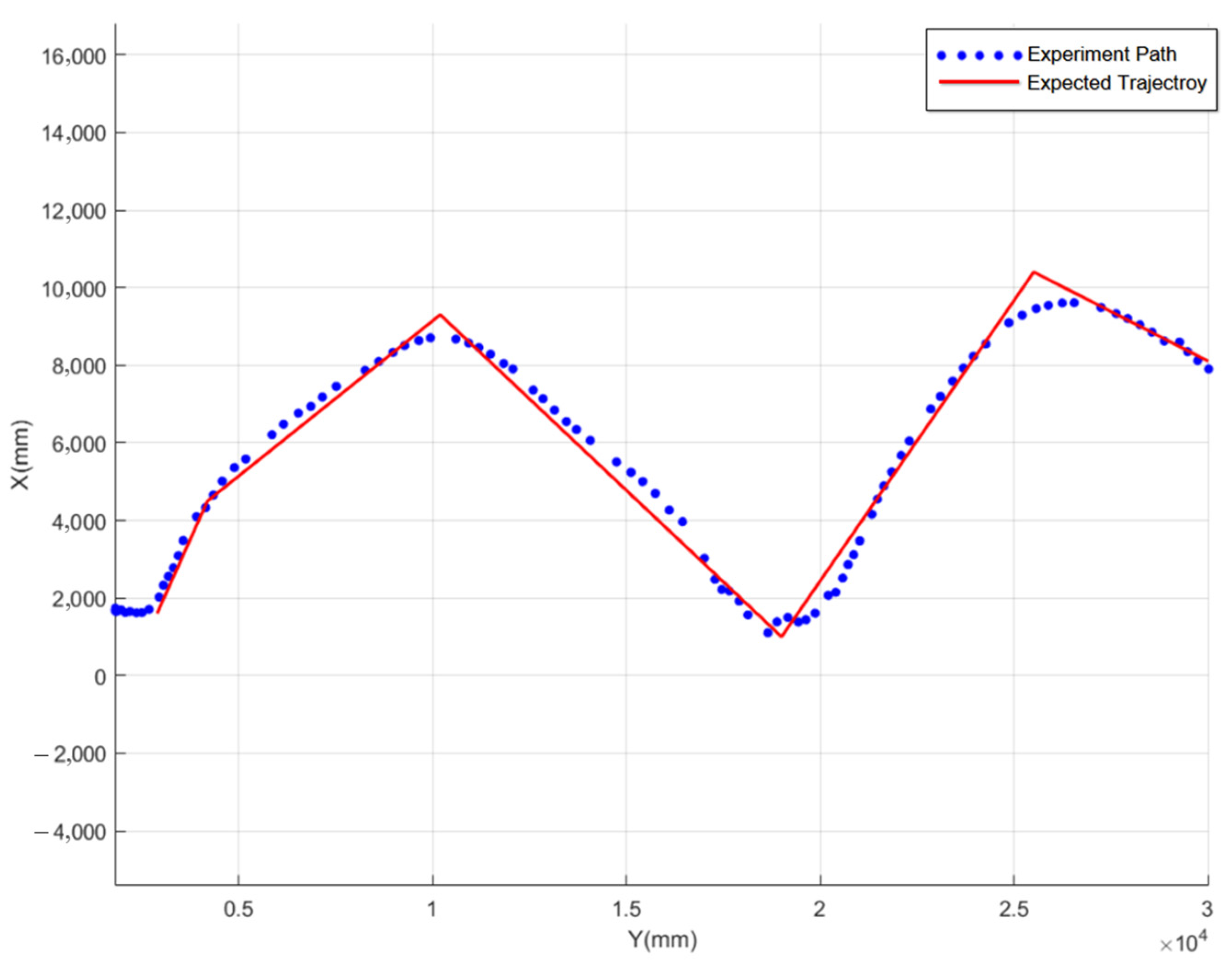
The experiment involved six irregular trajectory points. Initially, the propeller speed was adjusted in still water to achieve a USV speed of 0.8 [m/s], corresponding to a Froude number of 0.21. The USV’s heading was adjusted based on its real-time position relative to the first target point of the trajectory. Once the wave-making machine established a stable waveform with the desired amplitude and wavelength, intelligent control was activated on the host computer. The USV dynamically adjusted its rudder angle according to the algorithm, ensuring movement along the trajectory points. The aforementioned method was used to measure and record the motion data of the USV. The experimental process is depicted in
Figure 12, and the six trajectory points along with the USV’s motion trajectory are shown in
Figure 13.
The experiment demonstrated that, despite wave disturbances, the USV effectively tracked all trajectory points with a smooth path, achieving a maximum trajectory error of approximately 200 [mm]. This error is small and is primarily attributed to deviations in trajectory point acquisition caused by the UWB positioning accuracy and the resulting control deviations. Under the current hardware conditions and operating modes, the positioning accuracy was optimized using filtering techniques; however, it is still affected by equipment precision, UWB positioning methods, and electromagnetic interference from water waves and metal tracks in the tank. Despite these challenges, the experiment and error analysis indicate that the intelligent matching technique for control parameters based on the proposed method achieves an excellent control accuracy under existing conditions.
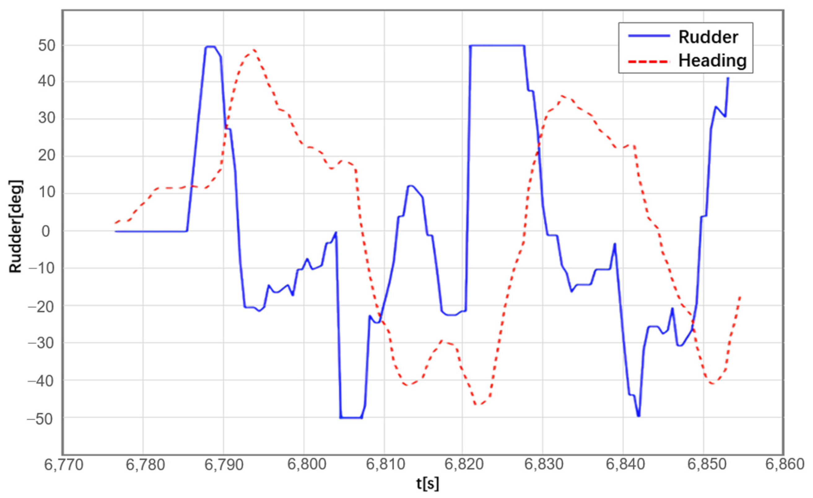
Figure 14 illustrates the real-time feedback of the rudder angle and the measured heading angle during the experiment. The changes in heading reveal five major trend adjustments required for path tracking, corresponding to the five segments in the actual trajectory. The heading changes were smooth, with a maximum rudder angle of 50 degrees at sharp turns along the target trajectory. The adaptive control yielded favorable results.
6. Conclusions
In this study, we present a novel algorithm that integrates DDPG with a PID controller to achieve path following in the presence of complex conditions, particularly wave interference. The algorithm begins by leveraging a 3-DOF MMG maneuvering motion model, which serves as the foundation for subsequent DDPG training. CFD simulations and regression analysis are employed to extract hydrodynamic derivatives and interaction coefficients necessary for precise motion prediction. We further detail the LOS guidance strategy, which directs the USV to follow a virtual target along the desired trajectory, with PID parameters adjusted dynamically via the DDPG framework.
The design of both the Actor and Critic networks is carefully structured, and to address the issue of slow training speeds in DDPG, we implement a dual-experience pool, separating the successful and failed experiences. Additionally, an adaptive batch size function is introduced to minimize data correlations, further enhancing the training efficiency. The reward function is rigorously formulated to account for both the lateral deviation and heading angle deviation, and its effectiveness is thoroughly examined under various operating conditions.
Simulations and experimental trials involving path following in Zigzag and turning maneuvers, conducted under wave disturbance, demonstrate the algorithm’s robust performance. The USV maintained superior tracking accuracy, even under continuously varying wave directions, highlighting the algorithm’s strong generalization capabilities and robustness.
Two key practical insights emerge from this work: First, the desired trajectory must align with the USV’s maneuvering limits. Trajectory points that exceed the USV’s steering capabilities, especially under full rudder conditions, will render the target trajectory unattainable in the presence of external disturbances. This not only compromises tracking performance but also hinders the Reinforcement Learning process. Second, while improving tracking accuracy, setting excessively small thresholds for error in the reward function can lead to instability in the neural network. Lowering the static error threshold makes successful experiences more difficult to achieve, thereby slowing the agent’s learning rate and significantly increasing the training time.
