Trajectory-Following Control of an Unmanned Aerial–Aquatic Vehicle under Complex Coupling Interferences

Abstract

This article explores trajectory-following control for an unmanned aerial–aquatic vehicle (UAAV) navigating complex ocean disturbances and the interplay of air–seawater coupling factors. First, leveraging the backstepping technology, an adaptive algorithm is proposed to tackle the attitude and position following. Additionally, a nonlinear observer is crafted to estimate complex ocean disturbances. The UAAV model, characterized by six degrees of freedom (DOF) and nonlinear properties, experiences significant pose changes when emerging from water, underscoring the critical importance of precise pose control. Finally, stability analysis and numerical simulations are demonstrated to verify the feasibility and validity of the proposed control strategies.

1. Introduction

Over the past few decades, the challenges associated with designing manned vehicles, characterized by complex layouts, high costs, and low efficiency, have prompted a rapid and distinct development of unmanned vehicles. This evolution is particularly notable in the realms of unmanned aerial vehicles (UAVs) and unmanned underwater vehicles (UUVs) [1,2,3]. To enhance the exploration and utilization of marine resources, as well as to meet military requirements, countries worldwide are consistently advancing diverse and innovative unmanned platforms [4]. Traditional UAVs typically operate within a single medium, posing challenges in adapting to the progressively complex task requirements. This led to the emergence of an amphibious air–water cross-media vehicle capable of efficiently functioning in two distinct media conditions.

Proposing the military four-in-one safety concept encompassing sea, land, air, and space as the ultimate frontier of security underscores the paramount importance of UAV development. This is particularly significant, with a spotlight on the recently introduced cross-medium vehicle concept [5,6]. On the civilian front, traditional underwater robots and drones deployed on ships face limitations, especially in tasks like marine resource surveys. The emergence of transmedia vehicles, however, provides a positive direction in this area. Additionally, the UAAV, as a cross-medium vehicle, offers a distinct advantage over underwater vehicles. It can transition into the air to reduce drag when high-speed travel is necessary [7]. Hence, maneuver control of cross-medium vehicle systems has evolved into a captivating subject, given its vast potential applications in missile launches, environmental monitoring, and submarine surfacing [8,9,10].

In terms of motion control, the UAAV performs alternating maneuvers in both air and water, resulting in abrupt changes in propeller forces and rudder moments. In reference [11], an aerodynamic and hydrodynamic model of angular motion was established for a transmedia vehicle featuring a quadrotor layout. Building upon this, a method was introduced for stabilizing water emergence control of a transmedia vehicle in the longitudinal plane. The study delves into the impacts of additional mass and inertial forces on the water emergence process during transmedia motion. Moreover, disturbances in the liquid and intricate collisions between the vehicle and the liquid can negatively impact the motion control of the UAAV, therefore compromising the stability and overall performance of the vehicle. During the execution of a water-exit maneuver, a trajectory tracking controller is established according to [12] to meet the requirements for a large-angle water outlet.

The backstepping control method proves more effective in addressing the nonlinearity issue in motion control [13,14,15]. Conversely, the adaptive control algorithm demonstrates a lesser sensitivity to changes in the model parameters of the controlled object. When combined with insights into control-method switching, the application of these methods to cross-medium vehicle control problems becomes profoundly significant for advancing research in cross-medium vehicle control.

The UAAV consistently contends with intricate external disturbances originating from wind, waves, and currents. Particularly at the water–air interface in oceans and lakes, it tends to be more susceptible to external environmental influences. Consequently, the maneuverability of the UAAV in such conditions is notably hampered by the coupling hydrodynamics. Throughout the water emergence process, the UAAV undergoes significant changes in fluid dynamics and is additionally influenced by external factors, notably wind and waves [16]. The critical stage for the UAAV is the exit phase at the water surface and air juncture, where the external environment is exceptionally complex, leading to inevitable interference. Therefore, considering these external interferences, ensuring effective maneuver control of the vehicle becomes imperative.

To enhance the control capabilities, a disturbance observer was developed specifically for the disturbances caused by wind and waves [17,18,19]. Building upon this, the environmental load associated with wind and waves in the subsequent moment was estimated and integrated into the vehicle’s controller, enabling the determination of the vehicle’s motion state. The interference observer not only assesses the external environmental load on the vehicle but also provides a level of compensation to enhance the controller’s resistance to interference. To align the control research of the vehicle with the real scenario during this stage, adjustments were made to the kinematics and dynamics models of the vehicle in the exit phase. The interference forces and torques acting on the vehicle were meticulously analyzed and modeled [20]. This paper concentrates on the vehicle’s exit stage, where a trajectory tracking controller is designed. The interference estimation results are then compared with pre-designed interference to evaluate the interference estimator’s effectiveness. Finally, simulation verification of the motion control process is conducted.

Currently, there is a scarcity of studies addressing maneuver control issues for UAAVs that account for complex disturbances at the air–seawater interface. The primary challenge in this domain lies in the fact that the unknown and intricate environment can hinder the vehicle’s proper and smooth movement. Notably, the UAAV may experience thrill, leading to the unstable movement of the entire system. In response to these challenges, this article introduces an adaptive backstepping control algorithm integrated into a disturbance observer scheme for the UAAV system, considering the presence of coupling disturbances. In comparison to existing works, the innovations of this study can be summarized as follows:

(1) We will introduce an adaptive backstepping control scheme designed for the fixed-wing UAAV system. Unlike conventional backstepping approaches [14,15], our method dynamically accommodates changing system dynamics, enhancing its adaptability and performance in real-world applications. Moreover, the proposed control scheme exhibits remarkable robustness against complex coupling interferences, which holds significant importance in practical engineering applications. In contrast to PD control [11], backstepping control is a nonlinear technique that systematically addresses complex and nonlinear system dynamics. It employs a recursive design approach, developing the control law step by step, with a focus on canceling out nonlinearities and ensuring system stability.

(2) The kinematic and dynamic models of the UAAV are formulated by altering the order of Euler transformations to account for the motion characteristics during the water-exit process. Subsequently, the considerable nonlinearities and robust coupling inherent in the out-of-water phase, along with time-varying parameters, are addressed. The stability of UAAV control during the out-of-water motion phase was then verified.

(3) The disturbance force and moment resulting from wind and wave loads on the vehicle are analyzed and modeled. Given that the roll angle and bow angle can be approximated as small quantities, the fixed-wing cross-medium vehicle can be simplified as a 4-DOF model. Subsequently, a disturbance observer is designed to estimate wind and wave disturbance loads, which are then used as inputs for the external force of the UAAV dynamic system. Building upon the designed disturbance observer and controller, a mathematical model for wind and wave disturbances is established to facilitate stability analysis.

The structure for the remaining sections of this article is outlined as follows. Section 2 introduces the maneuvering model of the UAAV, encompassing both kinematic and kinetic models. Section 3 establishes models for external environmental disturbances, including winds and waves. The core processes of the motion control algorithm are detailed in Section 4. The effectiveness of the proposed control protocol is demonstrated through numerical simulations in Section 5. Finally, Section 6 provides concluding remarks.

2. The Maneuvering Model of UAAV

In this section, we will address a foundational concern by first presenting the kinematics and dynamics model of the UAAV. The kinematics and dynamics models of cross-medium vehicles can be categorized into three types based on the medium in which they operate: the underwater movement stage, the air flight stage, and the cross-medium emergence stage. In particular, the cross-medium emergence stage holds significance for the entire maneuver mission, serving as a cornerstone for subsequent research on control methods for cross-medium vehicles.

2.1. The Kinematic Model of UAAV

This subsection primarily delves into the motion modeling of the cross-medium vehicle, emphasizing that a well-founded motion model serves as the bedrock for subsequent research on control methods. The UAAV represents a novel aircraft capable of navigating in both air and underwater environments. Moreover, the precision of the motion model establishment directly impacts the accuracy of subsequent issues such as attitude control, speed control, and trajectory tracking. The kinematics and dynamics models of cross-medium vehicles are categorized based on the medium in which they operate, including the underwater movement stage, the air flight stage, and the cross-medium exit stage.

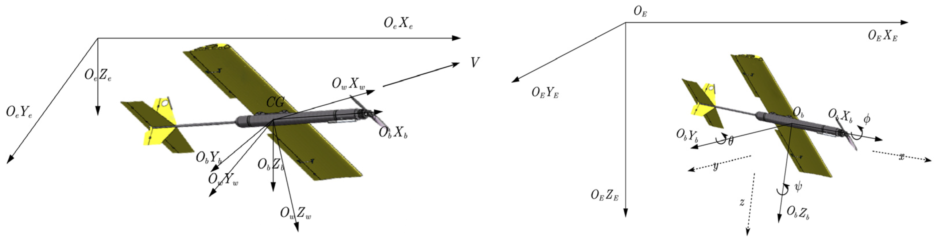
Modeling the UAAV system encompasses understanding both its dynamics and statics. Statics involves the equilibrium of the vehicle under uniform velocity or at a stationary position, while dynamics pertains to the accelerated motion of the vehicle. Kinematics focuses on the geometrical aspects of the vehicle’s motion, whereas kinetics addresses the forces responsible for the motion of the UAAV. Consequently, the motion of the UAAV in geodetic and body coordinate systems is illustrated in Figure 1.

Where $O_b-X_b{Y}_b{Z}_b$ represents the body coordinate system, $O_E-X_E{Y}_E{Z}_E$ represents the geodetic coordinate system, $O_w-X_w{Y}_w{Z}_w$ represents the velocity coordinate system.

In the delineation of the aforementioned coordinate system, the six degrees of freedom of the vehicle are described, encompassing both translational and rotational motion. The underwater gliding of the vehicle and the description of its six degrees of freedom movement can be referenced using the symbol system of the International Towing Tank Conference (ITTC) and the Society of Naval Architecture and Marine Engineering (SNAME) [21]. In particular, the motion model can be described as

$$\dot{\mathit{\eta }}=\mathit{J}\left(\mathit{\eta }\right)\mathit{v}$$

(1)

where $\mathit{J}(\eta )$ stands for the rotation matrix between $O_E-X_E{Y}_E{Z}_E$ and $O_b-X_b{Y}_b{Z}_b$, which is defined by:

$$\mathit{J}(\eta )=\left[\begin{array}{cccccc}\mathrm{c}\theta \mathrm{c}\psi -\mathrm{s}\varphi \mathrm{s}\theta \mathrm{s}\psi & -\mathrm{c}\varphi \mathrm{s}\psi & \mathrm{s}\theta \mathrm{c}\psi +\mathrm{s}\varphi \mathrm{c}\theta \mathrm{s}\psi & 0& 0& 0\\ \mathrm{c}\theta \mathrm{s}\psi +\mathrm{s}\varphi \mathrm{s}\theta \mathrm{c}\psi & \mathrm{c}\varphi \mathrm{c}\psi & \mathrm{s}\theta \mathrm{s}\psi -\mathrm{s}\varphi \mathrm{c}\theta \mathrm{c}\psi & 0& 0& 0\\ -\mathrm{c}\varphi \mathrm{s}\theta & \mathrm{s}\varphi & \mathrm{c}\varphi \mathrm{c}\theta & 0& 0& 0\\ 0& 0& 0& \mathrm{c}\theta & 0& \mathit{s}\theta \\ 0& 0& 0& \mathrm{s}\theta \mathrm{t}\varphi & 1& -\mathit{c}\theta \mathit{t}\varphi \\ 0& 0& 0& -\mathrm{s}\theta /\mathrm{c}\varphi & 0& \mathit{c}\theta /\mathit{c}\varphi \end{array}\right]$$

(2)

$\eta ={\left[{\eta }_1 {\eta }_2\right]}^{\mathrm{T}}$ is used to describe the position of the UAAV. $\dot{\eta }={\left({\dot{\eta }}_1 {\dot{\eta }}_2\right)}^{\mathrm{T}}$ denotes the velocity in the global coordinate system. ${\dot{\eta }}_1={\{\dot{x} \dot{y} \dot{z}\}}^{\mathrm{T}}$ stands for the linear velocity and ${\dot{\eta }}_2={\left\{\dot{\varphi } \dot{\theta } \dot{\psi }\right\}}^{\mathrm{T}}$ represents the rate of change in the Euler Angle. $v={\left(v_1 v_2\right)}^{\mathrm{T}}$ denotes the velocity in the body coordinate system, $v_1={\left\{u v w\right\}}^{\mathrm{T}}$ stands for the linear velocity, and $v_2={\left\{p q r\right\}}^{\mathrm{T}}$ represents the rotating angular velocity. $s,c,t$ denote the $\sin$, $\cos$, $\tan$, respectively. More specifically, $x y z$ express the linear displacement of surge, sway, and heave direction, respectively. $\varphi ,\theta ,\phi$ show the rotation angle in the above three directions. $u,\vartheta ,\omega .$ express the corresponding angular spin rate.

2.2. The Dynamics Model of UAAV

Professor Fossen [22] from Norway proposed a simplified version in vector form for the dynamic equation of six degrees of freedom for rigid bodies, which can be expressed as:

$$M_{RB}\dot{v}+C_{RB}\left(v\right)v={\tau }_{RB}$$

(3)

where $M_{RB}$ denotes the inertia matrix. $C_{RB}\left(v\right)$ represents the Coriolis force and centripetal force matrix. ${\tau }_{RB}={\left[X Y Z K M N\right]}^{\mathrm{T}}$ is the designed control force and moment, where $X Y Z$ is the longitudinal force, the lateral force, and the vertical force of the vehicle, and $K M N$ is the transverse moment, trim moment and yaw moment of the vehicle. Concretely, the inertia matrix can be expressed as follows:

$$M_{RB}=\left[\begin{array}{cc}\begin{array}{ccc}m& 0& 0\\ 0& m& 0\\ 0& 0& m\end{array}& \begin{array}{ccc}0& m{z}_G& -m{y}_G\\ -m{z}_G& 0& m{x}_G\\ m{y}_G& -m{x}_G& 0\end{array}\\ \begin{array}{ccc}0& -m{z}_G& m{y}_G\\ m{z}_G& 0& -m{x}_G\\ -m{y}_G& m{x}_G& 0\end{array}& \begin{array}{ccc}{I}_x& -I_{xy}& -I_{xz}\\ -I_{yx}& I_y& -I_{yz}\\ -I_{zx}& -I_{zy}& I_z\end{array}\end{array}\right]$$

(4)

where $M_{RB}$ satisfies the symmetric property and is a constant matrix, i.e., $M_{RB}=M_{RB}^{\mathrm{T}}>0,{\dot{M}}_{RB}=0$. Additionally, the Coriolis force matrix also can be shown as follows:

$$\begin{array}{r}{C}_{RB}(v)=[\begin{array}{ccc}0& 0& 0\\ 0& 0& 0\\ 0& 0& 0\\ -m\left(y_{G}q+z_{G}r\right)& m\left(y_{G}p+w\right)& m\left(z_{G}p-v\right)\\ m\left(x_{G}q-w\right)& -m\left(z_{G}r+x_{G}p\right)& m\left(z_{G}q+u\right)\\ m\left(x_{G}r+v\right)& m\left(y_{G}r-u\right)& -m\left(x_{G}p+y_{G}q\right)\end{array}\\ \begin{array}{ccc}m\left(y_{G}q+z_{G}r\right)& -m\left(x_{G}q-w\right)& -m\left(x_{G}r+v\right)\\ -m\left(y_{G}p-w\right)& m\left(z_{G}r+x_{G}p\right)& -m\left(y_{G}r-u\right)\\ -m\left(z_{G}p-v\right)& -m\left(z_{G}q+u\right)& m\left(x_{G}p+y_{G}q\right)\\ 0& -I_{yz}q-I_{xz}p+I_{z}r& I_{yz}r+I_{xy}p-I_{y}q\\ I_{yz}q+I_{xz}p-I_{z}r& 0& -I_{xz}r-I_{xy}q+I_{x}p\\ -I_{yz}r-I_{xy}p+I_{y}q& I_{xz}r+I_{xy}q+I_{y}q& 0\end{array}]\end{array}$$

(5)

3. External Environmental Disturbance

The impact of wind and waves on the control of the cross-medium vehicle during movement involves two primary aspects. First, during takeoff at a large angle in the exit strategy, the vehicle is susceptible to the effects of wind and waves. In this process, the vehicle approaches a vertical state, and the interference from waves and wind on the broad wing and shape results in significant disruptions during the water discharge process. Second, the body’s center of buoyancy changes with the fluctuation of draft caused by wave action, adversely affecting the vehicle’s attitude to stay above the water.

3.1. Wind Force Model

The disturbance force and torque induced by the wind load on the vehicle in the wind field can be calculated using the following equation:

$$\begin{gathered} f_{d,wind}=-\mathrm{sign}\left(v_{\mathrm{r}}\right)·C_{d,wind}·v_{\mathrm{r}}^2 \\ {\tau }_{d,\mathrm{wind}}=r_{wp}\times f_{d,wind} \end{gathered}$$

(6)

where $v_r=\left(v_1+v_2\times r_{\mathrm{wp}}\right)-R^{\mathrm{T}}{v}_w$ is the relative velocity of the vehicle body and the wind field at the center of wind pressure. $v_1$ is the linear velocity of UAAV, $v_2$ is the relative angular velocity, $R^{\mathrm{T}}$ is the rotation matrix of the vehicle from the inertial frame to the body coordinate system. $C_{d,wind}$ is the wind drag coefficient, representing the degree of influence of wind load on the resistance of the vehicle in the direction of the three axes of the UAAV system.

3.2. Wave Force Model

Drawing from the literature on linear wave theory [23], the load resulting from linear waves can be computed using pertinent knowledge from fluid mechanics [24]. The wave load on the cylindrical body and wing of an aircraft can be determined by the velocity potential function, wave surface function, and wave surface pressure distribution function corresponding to the characteristics of small amplitude long wave:

$$\Phi =\frac{{\zeta }_{a}g}{{\omega }_w}{e}^{-k_{w}z}\sin \left({\omega }_{w}t-k_{w}x\right)$$

(7)

$$\zeta =-{\zeta }_a\cos \left({\omega }_{w}t-k_{w}x\right)$$

(8)

$$p_{dyn}=-{\rho }_{water}\frac{\partial \Phi }{\partial t}$$

(9)

where ${\zeta }_a$ is the wave height relative to the horizontal plane $z=0$ in the inertial coordinate system, ${\omega }_w$ is the circular frequency unit of a wave is $\mathrm{rad}·{\mathrm{s}}^{-1}$; $k_w=2\pi /\lambda$ is the wavenumber of a wave, representing the wavenumber in each period with wavelength being $\lambda$; The circular frequency ${\omega }_w$ and wave number $k_w$ of a wave satisfy the dispersion relation $k_w={\omega }_w^2/g$ under wireless water depth.

Given the considerably small scale of the UAAV in comparison to the long peak waves of the ocean, the impact of loads resulting from incident waves can be disregarded [25]. The wave loads are primarily governed by the Froude-Krylov force, representing the perturbation force on an object under wave loading. This force is obtained through unit element re-integration when the wave pressure field is not influenced by the object in turn. Consequently, the disturbance force and moment due to wave loads on the vehicle can be calculated using the following equation:

$$f_{d,wave}=-{\displaystyle \underset{S_w}{\iint }{p}_{dyn}\overline{n}}dS$$

(10)

$${\tau }_{d,wave}=-{\displaystyle \underset{S_w}{\iint }\partial r\times \left(p_{dyn}\overline{n}dS\right)}$$

(11)

where $dS$ indicates that the UAAV is in the middle of a wave; $S_w$ denotes the wet surface area of the vehicle in the wave; $\overline{n}$ denotes the outward normal vector of the microelement; $\partial r$ denotes the spatial position of the microelement in the inertial coordinate system.

Up to this point, the interference force caused by wind and wave loads on the UAAV can be expressed using Equations (6) and (10), while the interference moment is expressed by Equations (7) and (11). Subsequently, the interference force and moment resulting from the corresponding assumed wave loads can be obtained using the following equation:

$$f_d=f_{d,wind}+f_{d,wave}$$

(12)

$${\tau }_d={\tau }_{d,wave}+{\tau }_{d,wind}$$

(13)

4. Control Algorithm Design

Given that the UAAV primarily focuses on positional quantities in the longitudinal plane during the water emergence process, the roll angle and bow angle can be approximated as small quantities, i.e., $\varphi =\psi =0$ and $p=r=0$. The kinematics and dynamics model can be simplified from Equations (1) and (3) to a mathematical model of longitudinal in-plane plus transverse displacement, i.e., a mathematical model of 4-DOF. The specific form of the state space can be expressed as:

$$\{\begin{array}{l}{\dot{x}}_1=f_1\left(x_1\right)x_2\hfill \\ {\dot{x}}_2=f_2\left(x_1,x_2\right)+Bu+d\hfill \\ y=x_1\hfill \end{array}$$

(14)

where $x_1={\left[x,y,z,\theta \right]}^{\mathrm{T}}$ is the state variable of the system, i.e., linear and angular displacements in the longitudinal plane in the geodetic coordinate system; $x_2={\left[u,v,w,q\right]}^{\mathrm{T}}$ are the first order state variables of the system, i.e., linear and angular velocities in the longitudinal plane of the body coordinate system; $y=x_1$ is the output of the system that indicates the position and attitude state of the vehicle. $u$ indicates the inputs to the control system, i.e., the inputs to the control forces and moments of the vehicle. $d$ indicates the disturbance of the control system. In this paper, the three phases use a unified disturbance to avoid the critical point in each phase of the control force, which appears to jump to ensure that the response of the control system is continuous. $B$ is the inverse of the quality matrix in the control system; $f_1\left(x_1\right)$ is the transformation matrix in the kinematic model equation in the case of 4-DOF, which is the transformation matrix of linear and angular velocities in the airframe coordinate system to the geodetic coordinate system position and attitude. $f_2\left(x_1,x_2\right)$ is the product of the inverse of the mass matrix in the control system and the forces and moments, including static forces: gravity and buoyancy, hydrodynamic forces: inertial and viscous forces [26], in addition to the control forces and moments, as well as the slight disturbance forces designed in this paper, i.e., $f_2\left(x_1,x_2\right)=M^{-1}\left(f_G+f_B+f_A+f_{\mu }+d\right)$.

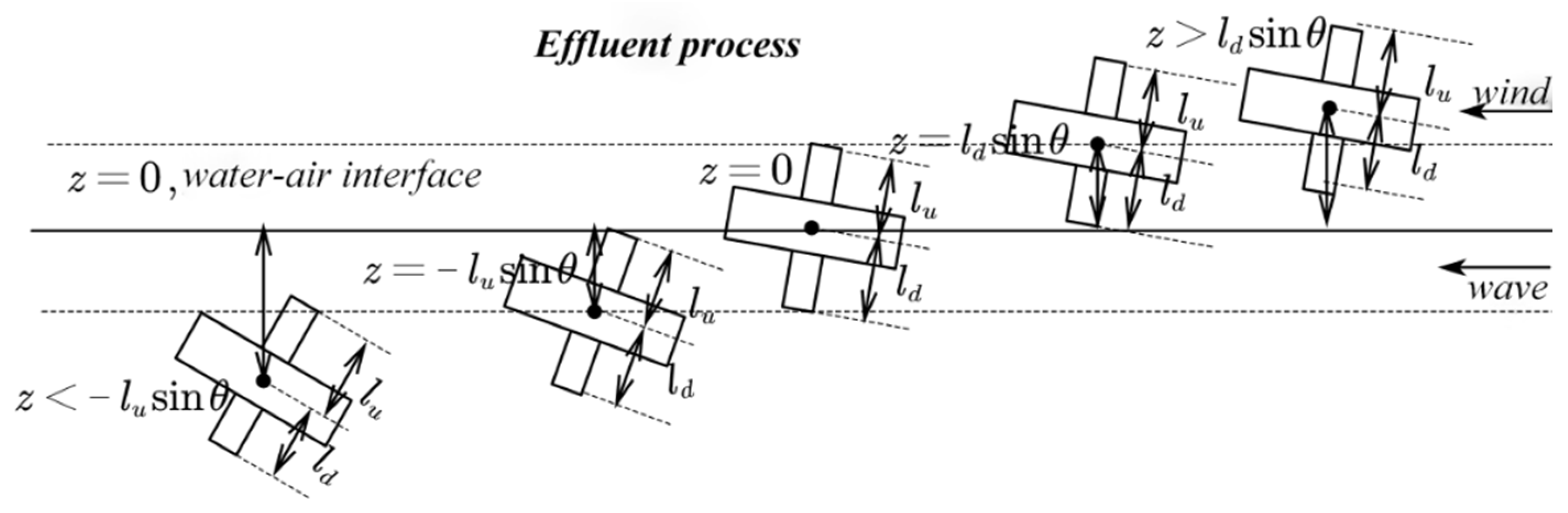
To facilitate a more effective analysis of the control laws during the out-of-water process, an equivalent approach is employed to conceptualize the navigator as comprising a cylindrical body and approximately rectangular wings. Define the distance from the center of mass to the upper and lower bottom surfaces as $l_u$ and $l_d$, respectively. $z$ is the height of the center of mass of the vehicle, defining $z=0$ as the interface between water and air; $z>0$ denotes air; $z<0$ denotes water. The emergent state is partly in the water and partly in the air and is expressed as a range of $z\in \left[-l_d\sin \theta ,l_u\sin \theta \right]$. The craft completely in the water is expressed as $z<-l_u\sin \theta$, and completely in the air is expressed as $z>l_d\cos \theta$. 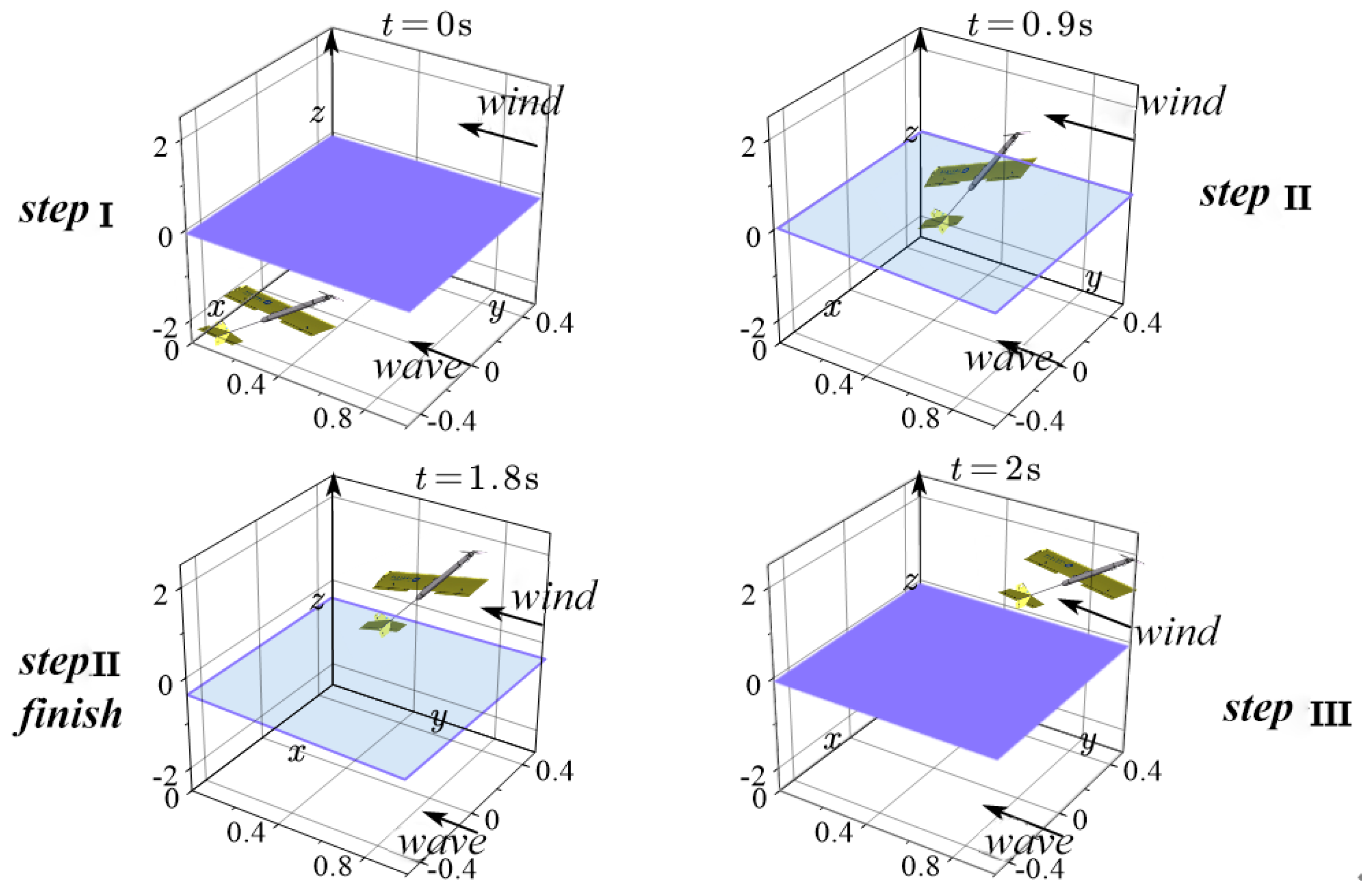Such situations are handled when the dynamics are written in a particular way, and a switched controller is designed [27] to tackle such dynamics. A schematic diagram of UAAV exiting the water across the medium in the presence of wind and wave disturbances is shown in Figure 2.

In what follows, the specific steps of the backstepping method of designing a control law will be stated.

Step 1: The error variable and Lyapunov function of the trajectory tracking controller are first defined as

$$e_1=x_1-x_{1d},V_1=0.5\ast e_1^2$$

(15)

where $x_{1d}$ denotes the desired exit trajectory of the navigator, for which the control system needs to guarantee a second-order continuously derivable; $V_1$ denotes the Lyapunov energy function of subsystem 1 used to determine whether the designed controller is asymptotically stable. Subsystem 1 is defined as

$${\dot{x}}_1=f_1\left(x_1\right){\alpha }_1$$

(16)

where ${\alpha }_1$ is the virtual control law and can be designed as

$${\mathit{\alpha }}_1=f_1^{-1}\left(x_1\right)\left(-k_1{\mathit{e}}_1+{\dot{\mathit{x}}}_{1d}\right)$$

(17)

where $k_1$ is the designed control parameter and satisfy $k_1>0$.

Define the new error variable $e_2=x_2-{\alpha }_1$, the derivative of the Lyapunov function of the system can be calculated as

$$V_1=e_1{\dot{e}}_1=-k_1{e}_1^2+f_1\left(x_1\right)e_1{e}_2$$

(18)

The asymptotic stability of the controller requires that the Lyapunov function be negatively determined, so the new error variable must be zero, and the design of the controller subsystem 2.

Step 2: Define the new error variable $e_2$ and the corresponding Lyapunov function as

$$e_2=x_2-{\alpha }_1,V_2=V_1+0.5e_2^2=0.5\left(e_1^2+e_2^2\right)$$

(19)

On the premise of ignoring the disturbance force, the actual system will be established. In the subsequent nonlinear disturbance, the observer will give the disturbance on the UAAV:

$${\dot{x}}_2=f_2\left(x_1,x_2\right)+Bu$$

(20)

Thus, the actual control law is designed as

$$\begin{gathered} u=B^{-1}\left(-k_2{e}_2-f_2\left(x_1,x_2\right)+{\dot{\alpha }}_1+f_1\left(x_1\right)e_1\right) \\ =M_{\eta }\left(\eta \right)\left(-k_2{e}_2-f_2\left(x_1,x_2\right)+f_1^{-1}\left(x_1\right)\left(-k_1{\dot{e}}_1+{\ddot{x}}_{1d}\right)+f_1\left(x_1\right)e_1\right) \end{gathered}$$

(21)

where $k_2$ is the designed control parameter and satisfy $k_2>0$ and the dimensions of the column matrix are related to the system.

Substituting the above-proposed controller into the Lyapunov function $V_2$, yields

$$\begin{array}{l}{\dot{V}}_2=-k_1{e}_1^T{e}_1+e_1^T{f}_1(x_1)e_2+e_2^T(f_2(x_1,x_2)+Bu)-e_2^T{\dot{\alpha }}_1\\ =-k_1{e}_1^T{e}_1-k_2{e}_2^T{e}_2\\ \le -K{V}_2\end{array}$$

(22)

where $K=\min \left\{2k_1,2k_2\right\}$.

To proceed, the Lyapunov function $V_2=0.5\left(e_1^2+e_2^2\right)$ of the actual system is satisfied to be negative definite, and the control law designed based on the backstepping method satisfies the asymptotic stabilization requirement of the closed-loop system.

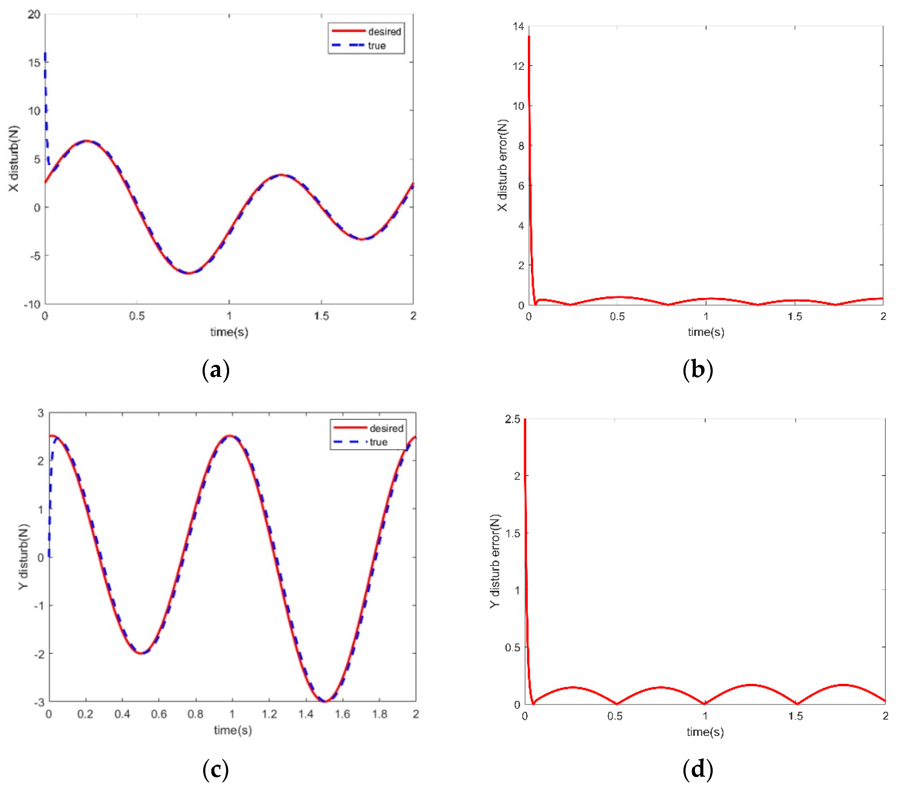
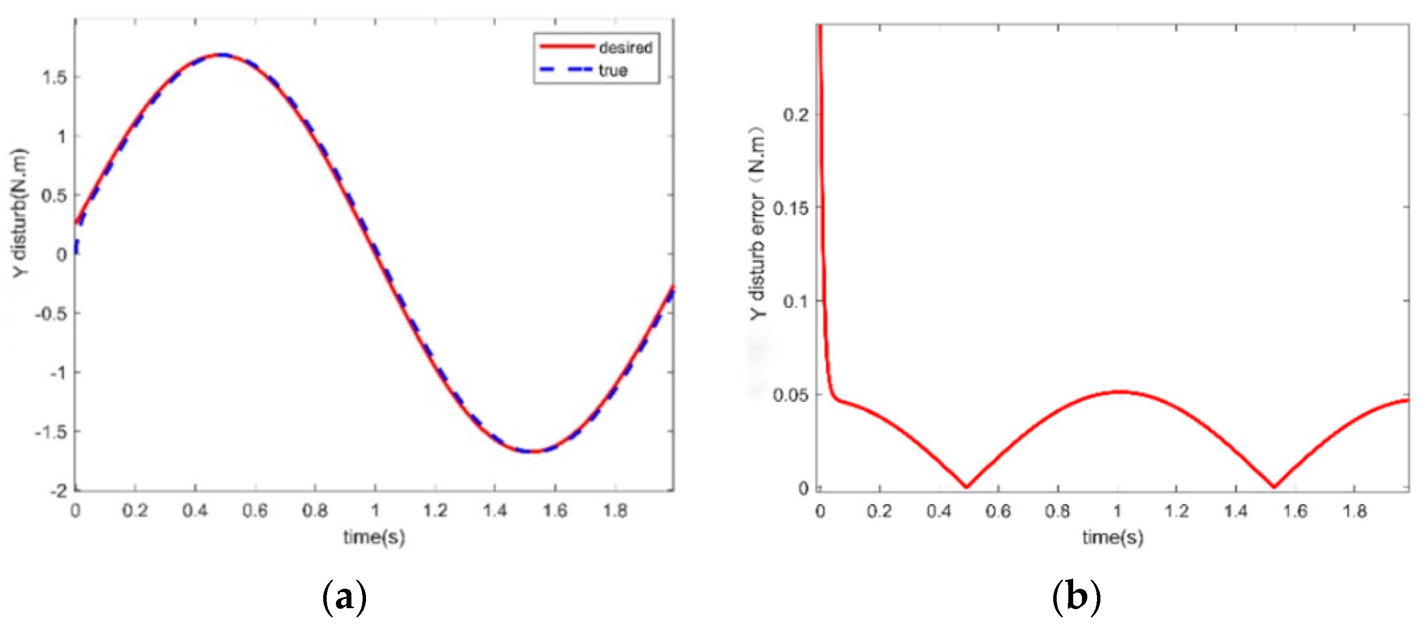
In what follows, the nonlinear disturbance observer will be established to estimate the interference forces and moments near the surface. Designing a nonlinear disturbance observer to estimate the effect of near-surface disturbances on the control system as follows:

$$\widehat{d}=\chi +p(x_1,x_2)$$

(23)

with

$$\dot{\chi }=-L(x_1,x_2)\chi +L(x_1,x_2)\left(G\left(x_1,x_2\right)-Bu-p(x_1,x_2)\right)$$

(24)

$$p(x_1,x_2)=c\left[\begin{array}{c}{\dot{x}}_{11}\\ {\dot{x}}_{11}+{\dot{x}}_{12}\end{array}\right]$$

(25)

in which $L(x_1,x_2)$ and $G(x_1,x_2)$ can be obtained by

$$L(x_1,x_2)f_1^{-1}(x_1){\ddot{x}}_1=\left[\begin{array}{cc}\frac{\partial p(x_1,x_2)}{\partial x_1}& \frac{\partial p(x_1,x_2)}{\partial {\dot{x}}_1}\end{array}\right]\left[\begin{array}{c}{\dot{x}}_1\\ {\ddot{x}}_1\end{array}\right]$$

(26)

$$G(x_1,x_2)=-f_1^{-1}(x_1){\dot{f}}_1(x_1)x_2-f_2(x_1,x_2)$$

(27)

where $\widehat{d}$ denotes the observation of the system disturbance by the nonlinear disturbance observer; $f_2(x_1,x_2)$ is the nonlinear term; $c$ is a large enough control parameter that can be adjusted by users. $x_{11}$ and $x_{22}$ satisfy $x_{11}={\left[\begin{array}{cc}x& y\end{array}\right]}^T$ and $x_{22}={\left[\begin{array}{cc}z& \theta \end{array}\right]}^T$.

Please see [28] for the convergence proof of the above observer.

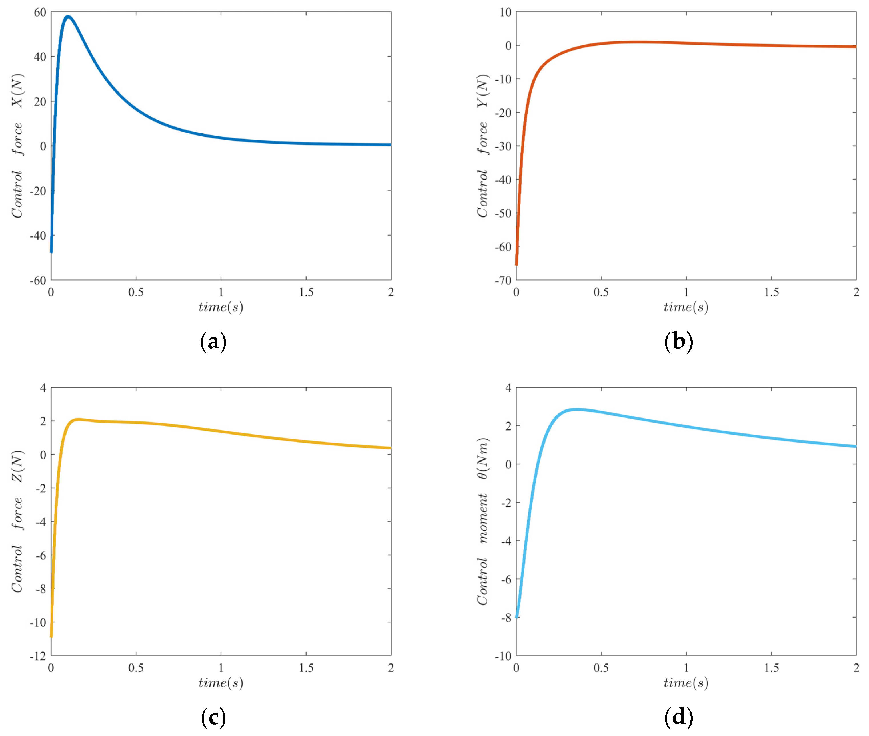
The controller is comprised of an inner loop for attitude control and an outer loop for position control. A nonlinear interferer is designed to estimate interference to the transmedia navigator, and the controller utilizes backstepping to achieve nonlinear control during the transmedia phase. Taking into account the coupling external handover interface disturbance, the final actual control law can be designed as follows:

$$\{\begin{array}{l}{\alpha }_1=f_1{\left(x_1\right)}^{-1}\left(-k_1{e}_1+{\dot{x}}_{1d}\right)\hfill \\ u=B^{-1}\left[-k_2{e}_2-f_2\left(x_1,x_2\right)-\widehat{d}+{\dot{\alpha }}_1^f-f_1^{\mathrm{T}}\left(x_1\right){\tilde{v}}_1\right]\hfill \end{array}$$

(28)

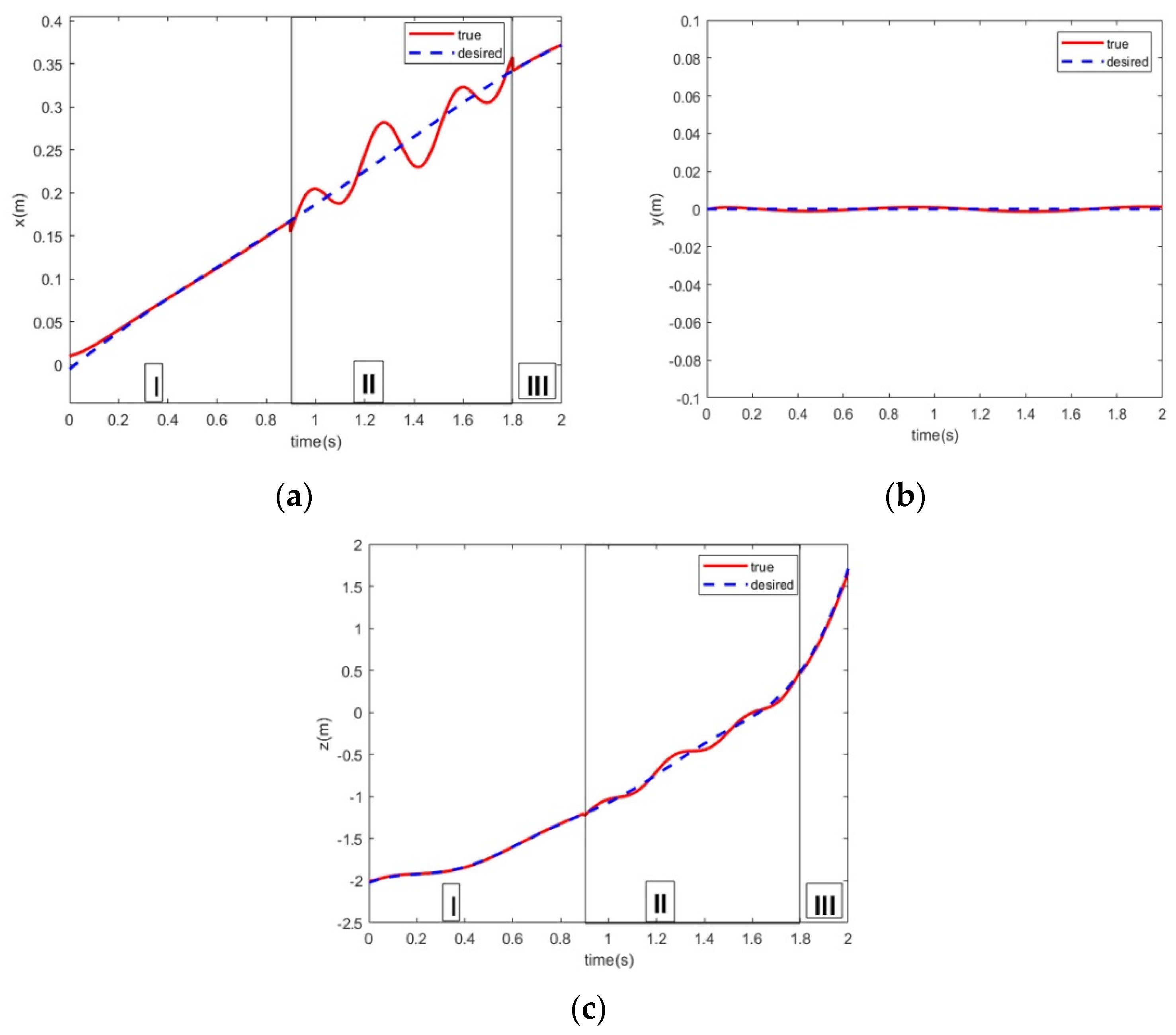
where $k_1$ and $k_2$ are the control parameters of the control law. Those are positive user-defined constants. $e_1$ and $e_2$ are the defining tracking error; ${\dot{x}}_{1d}$ is the derivative of the desired trajectory; $\widehat{\mathit{d}}$ is the estimates of nonlinear interference observers; ${\tilde{v}}_1$ and ${\tilde{v}}_2$ are the compensated tracking error. The design of the controller and control law for the UAAV in the out-of-water stage has been completed, laying the foundation for the subsequent motion control simulation.

Remark 1. 

For the designed control algorithm, the rule in parameter selections can be summarized as follows. According to the above theoretical analysis and the subsequent simulation experience, increasing $k_1$ and $k_2$ can improve the control accuracy and speed up the convergence, but also increase the control torque. Therefore, it is necessary to weigh the control performance, power consumption, and other indicators of the control system comprehensively.

Taking the derivative of $V_2$ and substituting the above-proposed controller into the Lyapunov function $V_2=\frac{1}{2}\left(e_1^T{e}_1+e_2^T{e}_2\right)$, yields

$$\begin{array}{ll}{\dot{V}}_2& =e_1^T{\dot{e}}_1+e_2^T{\dot{e}}_2\\ & =e_1^T\left(f_1(x_1){\alpha }_1+f_1(x_1)e_2-{\dot{x}}_{1d}\right)+e_2^T{\dot{e}}_2\\ & =-k_1{e}_1^T{e}_1+e_1^T{f}_1(x_1)e_2+e_2^T(f_2(x_1,x_2)+Bu+d)-e_2^T{\dot{\alpha }}_1\\ & =-k_1{e}_1^T{e}_1-(k_2-\frac{1}{2})e_2^T{e}_2+\Delta \\ & \le -\tilde{K}{V}_2+\Delta \end{array}$$

(29)

where $\tilde{K}=\min \left\{2k_1,2k_2-1\right\}$, $\Delta$ is the error resulting from the observer. Thus, it can be concluded that the error variable is stable. It is worth mentioning that the error converges to zero as long as $\tilde{K}{V}_2>\Delta$.

5. Numerical Simulation

For the UAAV described in (1) and (3), the trajectory tracking controller based on the disturbance observer adopts the same target trajectory to ensure that the vehicle can track the up-water trajectory under the disturbance of wind and wave loads, which is represented by the expected position and expected pitch angle. The actual combined wind and wave loads are designed as follows:

$$\{\begin{array}{l}{X}_{\mathrm{disturb}}=5\sin \left(2\pi ·t\right)+2.5\cos \left(\pi ·t\right)\hfill \\ Y_{\mathrm{disturb}}=2.5\cos \left(2\pi ·t\right)+0.5\sin \left(\pi ·t\right)\hfill \\ Z_{\mathrm{disturb}}=0.04\sin \left(3\pi ·t\right)+0.02\cos \left(0.5\pi ·t\right)\hfill \\ {\tau }_{\mathrm{disturb}}^{\mathrm{theta}}=1.5\sin \left(\pi ·t\right)+0.25\cos \left(0.5\pi ·t\right)\hfill \end{array}$$

(30)

5.1. Motion Control Simulation

The main content of this section is whether the desired trajectory of the predetermined vehicle can be tracked under the wave load shown in (30). Figure 3 shows the three-dimensional sequence diagram of the vehicle’s water emergence process under the disturbance of wind and wave loads.

Next, the expected trajectory is shown in (31)

$$\{\begin{array}{ll}{x}_d=\hfill & 2.264\sin \left(1.259t-0.3385\right)+1.98\sin \left(1.34t+2.755\right)\\ y_d=\hfill & 0\\ z_d=\hfill & 5.964\sin \left(1.993t-2.33\right)+47.18\sin \left(3.116t-0.02317\right)\\ & +43.15\sin \left(3.188t+3.064\right)+0.0819\sin \left(7.647t+2.479\right)\hfill \end{array}$$

(31)

In the above vehicle exit-water trajectory, the initial position of the vehicle is the key factor for the exit. The initial state of the vehicle is selected as $x_{d0}=0,y_{d0}=0,z_{d0}=-2 \mathrm{m}$, i.e., ${\eta }_{1d0}={\left[0 0 -2\right]}^{\mathrm{T}}$; The initial velocity is $v\left(0\right)={\left[0.169,0,0.1333\right]}^{\mathrm{T}}\mathrm{m}/\mathrm{s}$, Initial trim angle is ${\theta }_{d0}=0.698\mathrm{rad}$.

After many experiments in the simulation process, a set of parameters with better tracking effects is selected. Under environmental interference, the control parameters and the key parameters of the nonlinear function to be designed in the interference observer are $k_1=k_2=10$ and $c=50$. After the design of the above key parameters is completed, the motion control simulation under wind and wave load interference is carried out, and the simulation results are shown in Figure 4 and Figure 5.

In Figure 4, the position curve in the X-axis direction fluctuates and changes, mainly because the disturbed force in the emergence water stage is the superposition of disturbed force in the form of a sinusoidal curve, which is consistent with the real wave disturbance of the actual vehicle. In addition, the UAAV is in a state of large dip angle during the emergence process, which is greatly disturbed by wind and waves, resulting in the negative upward velocity along the X-axis and finally causing fluctuation.

The whole process of coming out of the water is divided into three stages: Stage 1 is when the vehicle is completely in the water, Stage 2 is when the vehicle is at the interface between water and air, and Stage 3 is when the vehicle is in the air, as shown in Figure 5a. At around 0.9 s, the propeller of the vehicle begins to emerge from the surface of the water, and at around 1.8 s, the vehicle is completely detached from the water, ending in two different medium states of water and air.

The simulation results reflect the position and attitude tracking of the vehicle in the process of water emergence. It can be concluded that the vehicle is significantly affected by wind and wave loads in the water emergence stage under the interference of wind and wave loads, and the tracking effect is better when the vehicle is in the single medium stage. The position diagram of the vehicle in three-dimensional space is shown in Figure 5b, which shows the change in the space position of the vehicle in three stages.

5.2. Simulation of Interference Estimation

Based on Equation (22), an estimation model was established to accurately estimate the disturbance force and torque of the vehicle in the process of water emergence and track the preset expected water emergence trajectory. The motion control simulation experiment of the vehicle under wind and wave interference is carried out to verify the position and attitude control performance of the designed controller under environmental interference. The simulation results of interference force estimation caused by wind and wave load of the vehicle in the process of water discharge are obtained, as shown in Figure 6. The estimated simulation results of the disturbance torque rotating around the Y-axis in the inertial coordinate system are shown in Figure 7.

As shown in Figure 6a,c,e, the simulation results of wind and wave load interference force estimation can reflect that the estimation results obtained by the designed interference observer are compared with the actual input interference force and torque. This reflects that the design of the interference controller can rapidly reduce the estimation error within 0.05 seconds. Figure 6b,d,f can be calculated, showing that after stabilization, the maximum error of the estimated results of the interference observer and the actual input results is less than 3%, indicating that the accuracy of the estimation of the interference observer is reasonable.

The simulation results of the disturbance torque estimation shown in Figure 7 can be analyzed and concluded. According to Figure 7a, it can be seen that the disturbance torque caused by wind and wave load is more accurate and responds faster than the disturbance force estimation. The error chart depicted in Figure 7b shows that compared with the force interference estimation, the initial error is smaller, and the time to reach the stable state of error is shorter.

The simulation results of the control signals shown in Figure 8 can be analyzed and concluded. According to Figure 8, it can be seen that the control signals are all bound and acceptable. Moreover, all the control signals have relatively large values at the beginning, and they converge to a small set with zero as the origin when the system is stable.

In summary, building upon the vehicle exit strategy, this section comprehensively addresses the control of the vehicle during the exit phase under the interference of wind and waves. It takes into account the impact of wind and wave interference estimated by the interference observation state and researches vehicle trajectory tracking.

6. Conclusions

The key contribution of this paper lies in tracking the water trajectory of a cross-medium vehicle when subjected to disturbances from wind and wave loads and estimating the disturbance using a disturbance observer. The process involves establishing a model for the disturbance force and moment caused by wind and wave loads. Subsequently, a disturbance observer is designed, and the impact of disturbance is incorporated based on the established dynamics model. Building upon this, the paper conducts simulations for the water emergence control of the UAAV under disturbance conditions, verifying the effectiveness of the designed controller in trajectory tracking amid disturbances. Finally, the disturbance force and torque on the vehicle due to wind and waves are estimated and validated, confirming the efficacy of the disturbance observer.

References

1. Chen, H.; Wang, X.; Li, Y. A survey of autonomous control for UAV. In Proceedings of the 2009 International Conference on Artificial Intelligence and Computational Intelligence, Shanghai, China, 7–8 November 2009; IEEE: Piscataway, NJ, USA, 2009; Volume 2, pp. 267–271. [Google Scholar]
2. Huang, B.; Zhang, S.; He, Y.; Wang, B.; Deng, Z. Finite-time anti-saturation control for Euler–Lagrange systems with actuator failures. ISA Trans. 2022, 124, 468–477. [Google Scholar] [CrossRef] [PubMed]
3. Huang, B.; Song, S.; Zhu, C.; Li, J.; Zhou, B. Finite-time distributed formation control for multiple unmanned surface vehicles with input saturation. Ocean Eng. 2021, 233, 109158. [Google Scholar] [CrossRef]
4. Kim, J.; Kim, S.; Ju, C.; Son, H.I. Unmanned aerial vehicles in agriculture: A review of perspective of platform, control, and applications. IEEE Access 2019, 7, 105100–105115. [Google Scholar] [CrossRef]
5. Wu, Y. Coordinated path planning for an unmanned aerial-aquatic vehicle (UAAV) and an autonomous underwater vehicle (AUV) in an underwater target strike mission. Ocean Eng. 2019, 182, 162–173. [Google Scholar] [CrossRef]
6. Wu, Y.; Li, L.; Su, X.; Gao, B. Dynamics modeling and trajectory optimization for unmanned aerial-aquatic vehicle diving into the water. Aerosp. Sci. Technol. 2019, 89, 220–229. [Google Scholar] [CrossRef]
7. Boniface, N. Design and Development of High Performance Unmanned Autonomous Aerial Vehicle (UAAV) Using MATLAB/Simulink in Civil Applications; Easy Chair: Manchester, UK, 2023. [Google Scholar]
8. Sujit, P.B.; Ghose, D. Optimal uncertainty reduction search using the k-shortest path algorithm. In Proceedings of the 2003 American Control Conference, Denver, CO, USA, 4–6 June 2003; IEEE: Piscataway, NJ, USA, 2003; Volume 4, pp. 3269–3274. [Google Scholar]
9. Biagini, M.; Corona, F.; Casar, J. Operational scenario modelling supporting unmanned autonomous systems concept development. In Proceedings of the Modelling and Simulation for Autonomous Systems: 4th International Conference, MESAS 2017, Rome, Italy, 24–26 October 2017; Revised Selected Papers 4. Springer International Publishing: Berlin/Heidelberg, Germany, 2018; pp. 253–267. [Google Scholar]
10. Wu, Y. A survey on population-based meta-heuristic algorithms for motion planning of aircraft. Swarm Evol. Comput. 2021, 62, 100844. [Google Scholar] [CrossRef]
11. Hernández-González, O.; Guerrero-Sánchez, M.-E.; Farza, M.; Ménard, T.; M’Saad, M.; Lozano, R. High gain observer for a class of nonlinear systems with coupled structure and sampled output measurements: Application to a quadrotor. Int. J. Syst. Sci. 2019, 50, 1089–1105. [Google Scholar] [CrossRef]
12. Ganesan, S.; Esakki, B. Computational fluid dynamic analysis of an unmanned amphibious aerial vehicle for drag reduction. Int. J. Intell. Unmanned Syst. 2020, 8, 187–200. [Google Scholar] [CrossRef]
13. Huang, B.; Zhou, B.; Zhang, S.; Zhu, C. Adaptive prescribed performance tracking control for underactuated autonomous underwater vehicles with input quantization. Ocean Eng. 2021, 221, 108549. [Google Scholar] [CrossRef]
14. Zhou, B.; Su, Y.; Huang, B.; Wang, W.; Zhang, E. Trajectory tracking control for autonomous underwater vehicles under quantized state feedback and ocean disturbances. Ocean Eng. 2022, 256, 111500. [Google Scholar] [CrossRef]
15. Li, Z.; Ma, X.; Li, Y. Robust trajectory tracking control for a quadrotor subject to disturbances and model uncertainties. Int. J. Syst. Sci. 2020, 51, 839–851. [Google Scholar] [CrossRef]
16. Guo, Y.; Liu, H.; Fan, X.; Lyu, W. Research progress of path planning methods for autonomous underwater vehicle. Math. Probl. Eng. 2021, 2021, 8847863. [Google Scholar] [CrossRef]
17. Xu, B.; Zhang, L.; Ji, W. Improved non-singular fast terminal sliding mode control with disturbance observer for PMSM drives. IEEE Trans. Transp. Electrif. 2021, 7, 2753–2762. [Google Scholar] [CrossRef]
18. Ye, J.; Roy, S.; Godjevac, M.; Reppa, V.; Baldi, S. Robustifying dynamic positioning of crane vessels for heavy lifting operation. IEEE/CAA J. Autom. Sin. 2021, 8, 753–765. [Google Scholar] [CrossRef]
19. Ye, J.; Roy, S.; Godjevac, M.; Baldi, S. Observer-based robust control for dynamic positioning of large-scale heavy lift vessels. IFAC-Pap. 2019, 52, 138–143. [Google Scholar] [CrossRef]
20. He, W.; Sun, Y.; Yan, Z.; Yang, C.; Li, Z.; Kaynak, O. Disturbance observer-based neural network control of cooperative multiple manipulators with input saturation. IEEE Trans. Neural Netw. Learn. Syst. 2019, 31, 1735–1746. [Google Scholar] [CrossRef] [PubMed]
21. Sname, T. Nomenclature for Treating the Motion of a Submerged Body through a Fluid; Society of Naval Architects and Marine Engineers: Alexandria, VA, USA, 1950; pp. 1–5. [Google Scholar]
22. Fossen, T.I. Guidance and Control of Ocean Vehicles. Doctor’s Thesis, University of Trondheim, Trondheim, Norway; John Wiley & Sons: Chichester, UK, 1999; ISBN 0471941131. [Google Scholar]
23. Hedges, T.S. An empirical modification to linear wave theory. Proc. Inst. Civ. Eng. 1976, 61, 575–579. [Google Scholar]
24. Toth, S.; Lake, B. Linear spin wave theory for single-Q incommensurate magnetic structures. J. Phys. Condens. Matter 2015, 27, 166002. [Google Scholar] [CrossRef]
25. Edition, F.; Journée, J.M.J.; Massie, W.W. Offshore Hydromechanics; Delft University of Technology: Delft, The Netherlands, 2001. [Google Scholar]
26. Zhou, B.; Huang, B.; Su, Y.; Wang, W.; Zhang, E. Two-layer leader-follower optimal affine formation maneuver control for networked unmanned surface vessels with input saturations. Int. J. Robust. Nonlinear Control 2023. [Google Scholar] [CrossRef]
27. Ye, J.; Roy, S.; Godjevac, M.; Baldi, S. A switching control perspective on the offshore construction scenario of heavy-lift vessels. IEEE Trans. Control Syst. Technol. 2020, 29, 470–477. [Google Scholar] [CrossRef]
28. Chen, W.-H.; Ballance, D.; Gawthrop, P.; O’Reilly, J. A nonlinear disturbance observer for robotic manipulators. IEEE Trans. Ind. Electron. 2000, 47, 932–938. [Google Scholar] [CrossRef]
Figure 1. Motion of UAAV in geodetic and body-fixed coordinate systems.
Jmse 12 00060 g001
Figure 2. Schematic diagram of the out-of-water phase.
Jmse 12 00060 g002
Figure 3. Three-dimensional time-series diagram of the water emergence process under wind and wave disturbances for cross-medium vehicles.
Jmse 12 00060 g003
Figure 4. Time response of positional trajectory tracking for out-of-water processes under environmental disturbances in transmedia vehicles. (a) X-axis position tracking results. (b) Y-axis position tracking results. (c) z-axis position tracking results.
Jmse 12 00060 g004
Figure 5. Schematic of attitude tracking time response and spatial 3D position of the cross-medium vehicle during water exit. (a) Simulation results of attitude tracking during the water-exit process. (b) Schematic diagram of the three-dimensional position tracking.
Jmse 12 00060 g005
Figure 6. Simulation results of interference force estimation for wind and wave loaded interference observer during the water emergence phase. (a) Estimation of wind and wave load disturbances in the X-axis. (b) Errors of disturbances estimation in the X-axis. (c) Estimation of wind and wave load disturbances in the Y-axis. (d) Errors of disturbances estimation in the Y-axis. (e) Estimation of wind and wave load disturbances in the z-axis. (f) Errors of disturbances estimation in the z-axis.
Jmse 12 00060 g006aJmse 12 00060 g006b
Figure 7. Simulation results of interference moment estimation for wind and wave loaded interference observer during the out-of-water phase. (a) Estimation of wind and wave disturbance moments around the Y-axis direction. (b) Error in estimation around Y-axis direction.
Jmse 12 00060 g007
Figure 8. Simulation results of control signals. (a) Control signal for x channel. (b) Control signal for y channel. (c) Control signal for z channel. (d) Control signal for θ channel.
Jmse 12 00060 g008
Disclaimer/Publisher’s Note: The statements, opinions and data contained in all publications are solely those of the individual author(s) and contributor(s) and not of MDPI and/or the editor(s). MDPI and/or the editor(s) disclaim responsibility for any injury to people or property resulting from any ideas, methods, instructions or products referred to in the content.