1. Introduction
Poor weather conditions, such as dense fog, heavy snow, and heavy rain, make it difficult to secure navigation routes, due to limited visibility. For example, during the five years from 2016 to 2020, there were 544 vessel accidents and 3652 casualties caused by sea fog in the Republic of Korea [
1]. Therefore, fog monitoring is important to prevent accidents on land and at sea [
2,
3], so that visibility meters are installed where vehicle traffic is heavy, such as in airports, major ports, and on highways. Visibility meters utilize optical sensors, which emit infrared rays and measure the amount of light source scattered in the atmosphere and the amount of light scattered by aerosols [
4]. Temperature sensors, humidity sensors, and other information aids the visibility estimates [
4].
Such advanced featured visibility meters are considerable expensive. However, serious errors exist in measured visibility data, in particular when the visibility data is measured at sea. Therefore, visibility data can be obtained by a well-trained observer, according to a guide from the World Meteorological Organization (WMO) [
5]. The Republic of Korea also has 23 observer measurement centers in different locations, although 291 places are measured by climate measurement systems [
6]. According to research in 2018 [
7], Lee compared the visibility data from trained observers and from visibility meters and the research found that visibility meters report more frequent fog and more dense fog, and this error is more obvious at sea compared to on land [
7]. For example, the measured data occasionally shows rapid changes in the intensity of fog, which is not an actual feature of a fog, as fog typically thickens gradually or weakens gradually. This causes a conflict of interest, e.g., frequent sea fog prevents ship operations, which effects people’s livelihoods, in particular the operators of small fishing vessels [
8]. Therefore, this paper proposes a method of estimating sea fog intensity using cameras rather than a visibility meter, since cameras provide identical visional information as human eyes do. Moreover, cameras are available at affordable prices so that the proposed algorithm can be rapidly applied and widely available. The proposed algorithm, called RDCP, provides more reliable visibility, in a way that is simple and easy to apply. The RDCP algorithm can be applied immediately to any type of existing cameras which are already mounted, without any additional costs, for sea fog and visibility estimation using the identical visional information as that received by observers.
Section 2 reviews the related literature, especially Dark Channel Prior (DCP), which is a fundamental component of the RDCP algorithm.
Section 3 explains the details of the RDCP algorithm and
Section 4 describes the experiments concerning RDCP and the results of this evaluation.
2. Literature Review
Image processing using cameras has been intensively studied for autonomous driving, drones, the defense industry, etc. The primary assumption of these studies is good weather conditions. Therefore, image processing in harsh weather conditions, such as at nighttime, in dense fog, during heavy rains, in storms, etc., is a separate study subject, and so this section reviews fog related research.
2.1. Fog Dehazing on Land
Dehazing or defogging algorithms have been developed in many studies, since fog has a significant influence on the performance of image processing algorithms. Dehazing studies can be categorized into two approach types. The first type increases the contrast of images; a mapping method according to pixel values (Xu, 2013) [
9] and an improved high boost algorithm (Ma, 2016) [
10] are in this category. The study in [
10] emphasizes the high frequency components of an image to enhance its clarity and contrast. This type of algorithm accurately restores the contrast of the image, which is degraded by fog; however, if the depth of the image is not properly considered, the contrast can be excessively increased. Here, the depth of an image is defined as the amount of color information contained in each pixel in an image. The second category estimates the depth of an image, e.g., Dark Channel Prior (DCP) (He, 2010) [
11], image-specific fusion (Wang, 2014) [
12], and a method using convolutional neural networks (Cai, 2016) [
13]. The study in [
13] utilizes deep learning to estimate depth information and utilize it for fog removal. This type of study estimates a transmission map or a depth map by considering both contrast and chromaticity, as well as visibility loss. However, these algorithms increase complexity and require greater computation volume.
2.2. Fog Dehazing in the Marine Enviornment
Fog removal algorithms on land and in a marine environment apply different approaches for dehazing. Fog removal studies on land consider geometric characteristics, such as roads, buildings and structures, and extract necessary data for fog removal from these environments. Fog removal studies in marine environments should consider complex optical phenomena, such as refraction and reflection of water, disturbance at sea level and in the air; therefore, fog removal in these environments is much more complex.
Hu (2019) [
14] proposes a light source decomposition algorithm to remove the light source-induced luminous effect from sea fog images and to recover objects covered by sea fog. First, the luminous effect of light from the input image is identified through a light source decomposition algorithm, and then light source information is extracted. This first step provides information about the origin and intensity of light and allows identification of the location and intensity of the light source that illuminates the object brightly. Next, the second step increases the visibility of the object by extracting the outline and details of the object covered by sea fog using separated light source information.
2.3. Sea Fog Visibility Estimation
For image processing studies related to fog images captured on land, dehazing is a major subject [
14,
15]. However, in terms of ocean fields, real-time visibility estimation is as important as dehazing. However, there are few studies on visibility estimation in sea fog images. Bae (2019) [
16] proposes a visibility estimation method combining DCP and the distance of a fixed object in a coastal area to estimate comprehensive visibility in a large area. Palvanov (2019) [
17] proposes a method of estimating visibility in sea fog images using a deep synthetic multiplication neural network. Most visibility estimation algorithms for ocean images are based on DCP, since the algorithm has long been verified and embedded in many different commercialized products, such as cameras for cars and CCTVs on roads. The next section discusses DCP in detail, along with some studies based on the DCL algorithm.
2.4. DCP
He [
11] proposes a light source decomposition algorithm, which removes the luminous effect on the light source from a fog image and recovers the object covered by the fog. The DCP algorithm is widely used in fog studies on land and in sea environments, and this algorithm can estimate visibility loss due to fog and effectively eliminate fog. DCP utilizes the fog model (Koschmieder, 1924) [
18] which is most commonly used to define the atmospheric scattering characteristics of fog images. The fog model is a mathematical model, which defines how fog scatters light and is used in different fog related studies.
While other existing algorithms require multiple images to remove fog, DCP is able to remove fog from a single image. However, a large amount of calculation is required to operate DCP, e.g., to relieve the blocking effect, additional techniques are added such as soft matting.
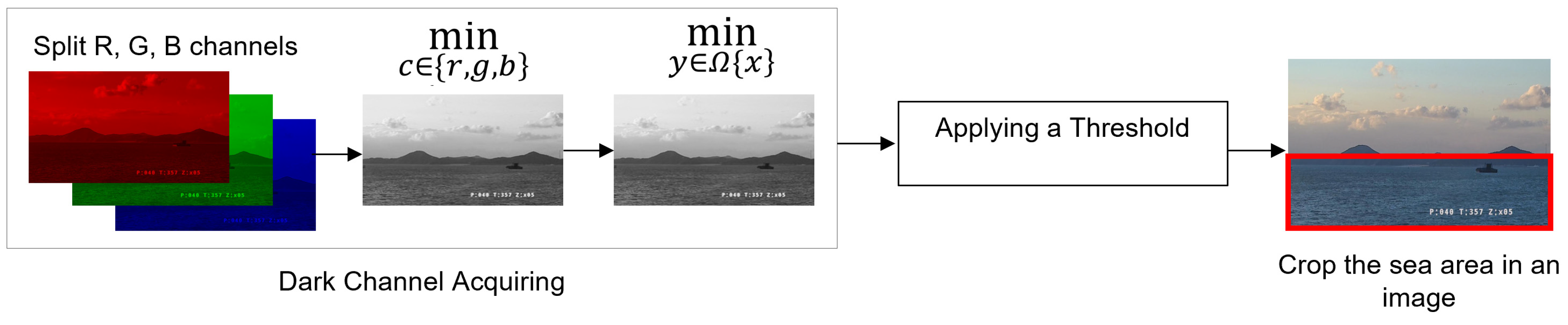
Figure 1 summarizes the main processes of DCP.
DCP uses an empirical assumption: in fog free images, most pixels tend to have very low brightness values in at least one of the three channels, i.e., Red (R), Green, (G), and Blue (B). As shown in
Figure 1, the first step of DCP is acquiring the Dark Channel (DC),
by (1), and
varies from 0 to 255
where
is a color channel,
represents
pixels, called local patch, centered at
, and
is a pixel in the local patch. The RDCP algorithm in this paper takes only the dark channel acquiring process of DCP, therefore further processes of DCP are not described here. Local patch size can vary depending on the size of the images; 15 × 15 is used in [
6] and the patch size is not a critical factor for the algorithm. In this paper, the experiments are conducted at 10 × 10.
There are many studies in restoring the visibility of images degraded by fog using the DCP algorithm. Huang (2014) [
19] proposed a technique to effectively overcome the visibility problem caused by fog by combining two main modules: the Haze Thickness Estimation (HTE) module and the Image Visibility Restoration (IVR) module. The HTE module is used to estimate fog thickening. It is effective in eliminating fog by identifying the loss of visibility due to fog and estimating the depth information of fog. The IVR module serves to restore the visibility of the image. This module solves the color problem caused by fog and the visibility problem of the image. It performs the process of improving the clarity and contrast of the image. Yang (2018) [
20] proposes estimation of the range of visibility, not by restoring fog. This study focuses on improving the DCP algorithm and estimating the range of visibility in combination with Grayscale Image Entropy (GIE) and Support Vector Machine (SVM). GIE is used in the field of image processing and computer vision, which is a statistical measurement method to measure image information, analyze the complexity of images, and measure the degree of disorder in the pixel value distribution of images. SVM is a supervised learning algorithm for classification and regression analysis used in the fields of machine learning and pattern recognition. These GIEs and SVMs are used to estimate the visibility of current road and traffic conditions and provide appropriate speed limits to improve traffic safety and reduce traffic congestion.
3. Reduced DCP
This paper proposes an algorithm called RDCP, which utilizes the initial step of DCP to estimate sea fog density and visibility. To estimate sea fog density in real-time, estimating from a single image is more helpful than processing multiple images, which means that DCP is suitable for the purpose of RDCP. However, DCP is a dehazing algorithm primarily for images on land and this implies significant calculations of DCP, which do not cause energy consumption problems, since the cameras are usually not battery operated on land. However, ocean facilities, such as buoys in the ocean environment, mostly operate under a highly limited power condition, therefore RDCP must estimate visibility while restricted to extremely low power supplies.
This study proposes using only the initial process of DCP because (1) we found the DC values of each pixel (
) are sufficient to estimate the sea fog density and visibility and (2) this leads to a reduction of algorithm complexity and computation requirements.
Figure 2 provides the diagram of RDCP. Here, DC value is defined in
Section 2.4 and (1) provides the equation for DC values. Further processes of RDCP are explained in the next subsections.
3.1. Applying a Threshold
The RDCP algorithm first acquires DC values ranging from 0 to 255 and uses these values for an index of fog intensity. DC values are compared in
Figure 3: the blue graph is a result of an image without sea fog in
Figure 4a, and the orange line with dense fog in
Figure 4b. Based on the empirical results of 320 images in four different locations, 100 is set as the threshold value in this paper. The possible DC values from 0 to 255 are applied by increasing in increments of 5. When 100 is applied, the difference in fog density achieves the most distinct results (results will be discussed in
Section 4.2). Therefore, 100 is chosen for the threshold value in this paper. In this example of the dense fog image (
Figure 4a), 44% of DC values are less than 100, whilst 1.4% of DC values of the no fog image (
Figure 4b) are more than 100. RDCP uses the percentage as a criterion of fog density, as it is clearly distinct according to fog density. The RDCP percentage is explained in (2).
3.2. Cropping a Sky Region
The disadvantage of DCP is that DCP does not work properly at sky regions in an image [
6], so the study manually cuts out the sky regions for the experiment dataset. Therefore, RDCP also crops the sky region from an image, which provides two primary benefits. First, it removes the ambiguity of DC values so that the estimation becomes more distinct according to the fog density. Second, it significantly decreases the number of pixels required for the calculation. There are various image processing algorithms to divide sea and sky in ocean images; however, this paper does not discuss cropping algorithms, since they are out of its scope. This paper uses the work of Jeon 2023 [
21] for the division of sky and sea regions in an image.
Figure 5 below provides an example of cropping only the sea area from the entire image.
4. Experiments and Evaluations
4.1. Experiment Datasets
Image-based fog studies usually use datasets of pairs of haze images and fog-free images for an identical scene. The datasets for research purposes usually use artificially synthesized images, since it is not easy to film and precisely pair them on-site. Most of these existing fog datasets are road images for autonomous vehicle research [
10]. As an example of a road synthetic fog dataset, Tarel (2012) [
22] proposes a paired dataset in which several types of fog are added to a virtual fog-free road composite image. Sakaridis (2018) [
23] applies a semantic segmentation method to the ground truth and different types of fog are synthesized to it.
However, in the case of sea fog studies, image datasets are very small in number and type compared to road image datasets. Therefore, this study uses raw image datasets, which are captured in real-time by cameras owned by the Korea Meteorological Administration Agency (KMAA) [
24] and the Korea Hydrographic and Oceanographic Agency (KHOA) [
25]. The images are captured from four different ports by cameras mounted on buoys. The four ports are located at Ganghwa Island, Pyeongtaek, Baengnyeong Island, and Ji Island and the locations are indicated in
Figure 6.
KMAA and KHOA also provide different data labels along with these images. The sea fog density labels are provided, and they are categorized as No-fog, Low-fog, Mid-fog, and Dense-fog.
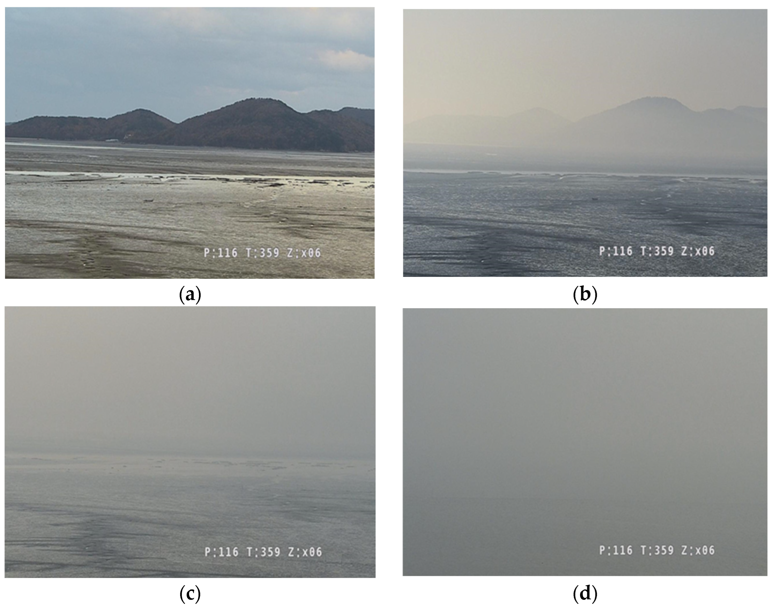
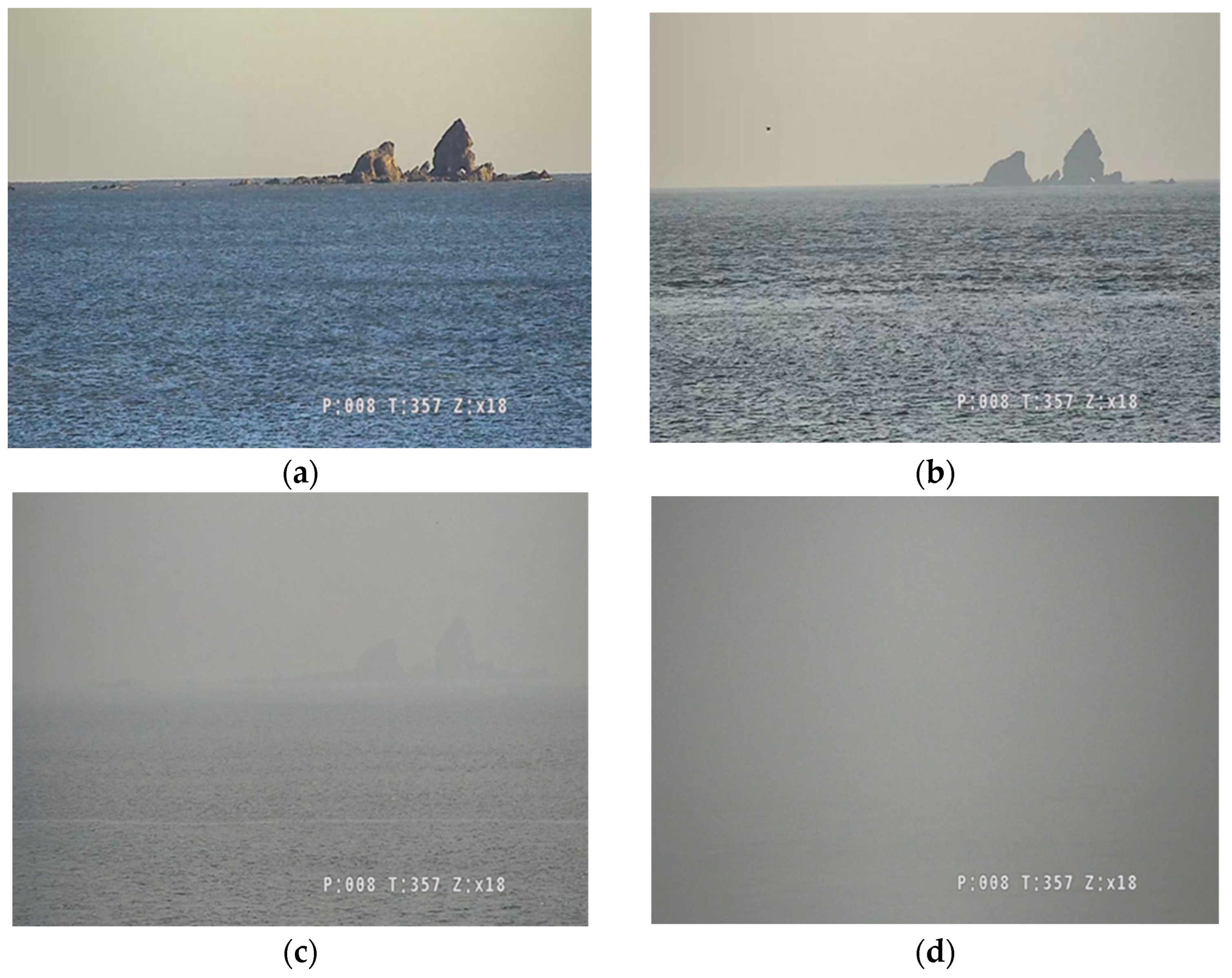
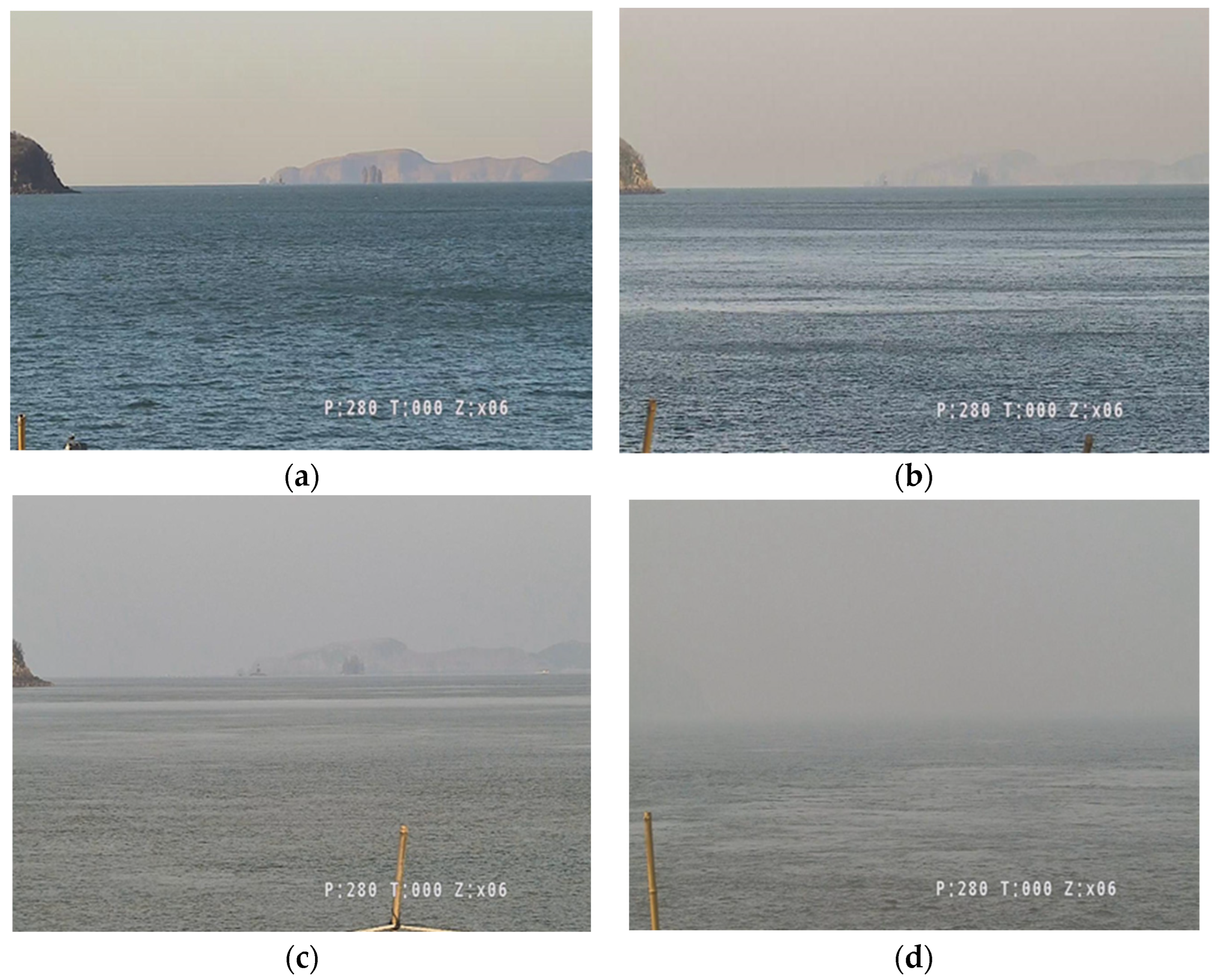
Figure 7,
Figure 8,
Figure 9 and
Figure 10 show example images having four different sea fog intensity labels at the four different locations. Other labels are also provided, such as temperature, humidity, pressure, visibility, wind direction, and water temperature. This paper chooses fog density and visibility labels to evaluate the performance of RDCP.
Table 1 compares the label values of the sea fog intensity and the visibility. To fairly evaluate the performance of RDCP using the labels, dense intensity estimation results of RDCP are equally defined into four categories.
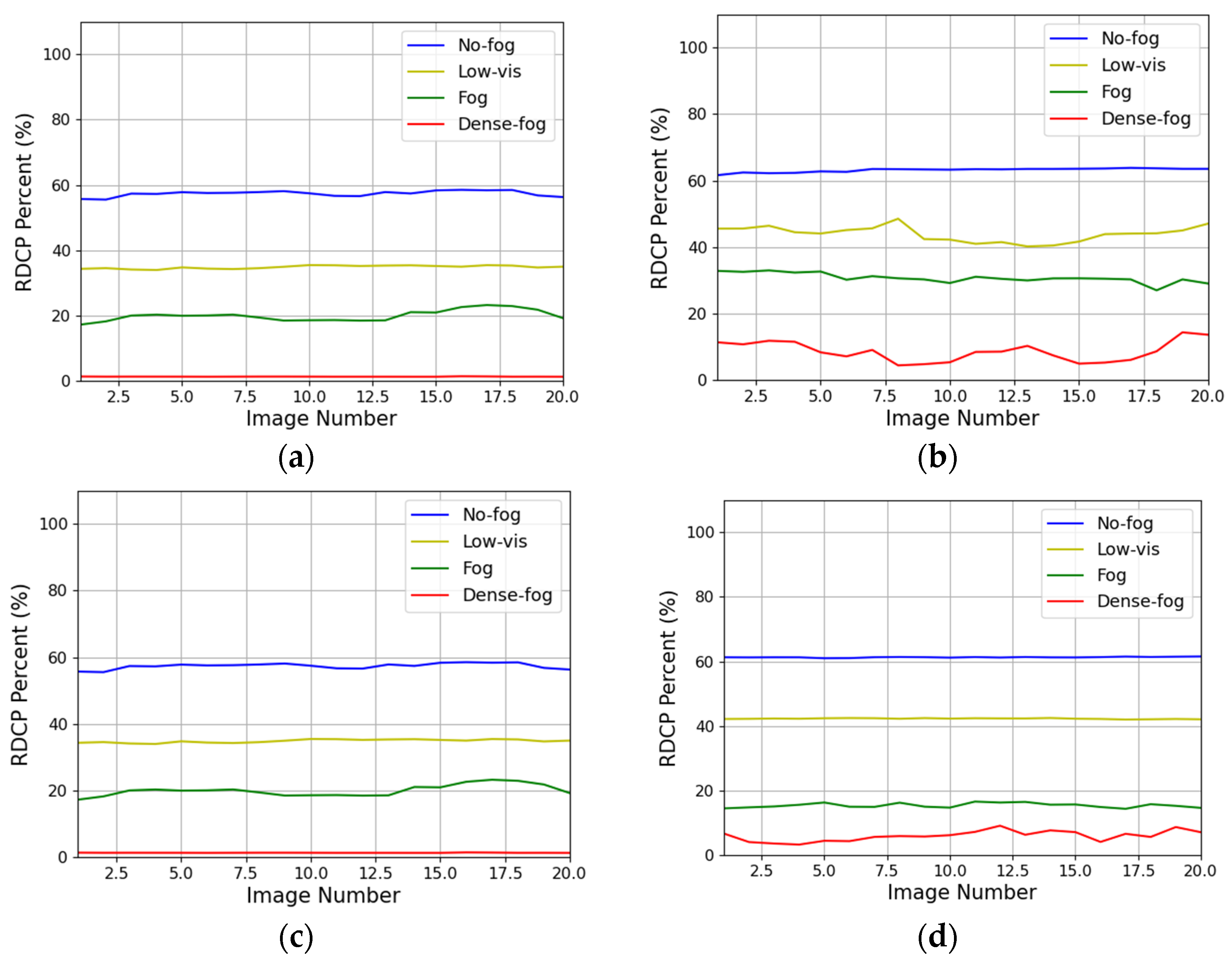
4.2. Sea Fog Intensity Estimation
To verify that the RDCP percentage of (2) can be a criterion of sea fog density, a total of 320 images is used. The size of all images is 1280 × 720 pixels. At each location, 20 images are selected for the four different fog intensity labels: 20 images for no-fog, 20 images for low-fog, 20 images for mid-fog, and 20 images for dense-fog. RDCP percentage values are calculated with each image and
Figure 11 shows the trends. The
X axis shows the number of images (i.e., 20 images) and the
Y axis shows the RDCP percentage value of each image.
As shown in
Figure 11, RDCP percentage values are fairly consistent according to the fog intensity, which implies that the RDCP percentage values have the potential to be used as a criterion of sea fog intensity. The graphs for no-fog (i.e., blue lines) represents the lowest intensity of sea fog and they have the largest RDCP values, with an average of 62.3%, since they have the highest number of pixels, which are smaller than the threshold. In this manner, the higher the intensity of sea fog, the lower the RDCP percentage values are in
Figure 11.
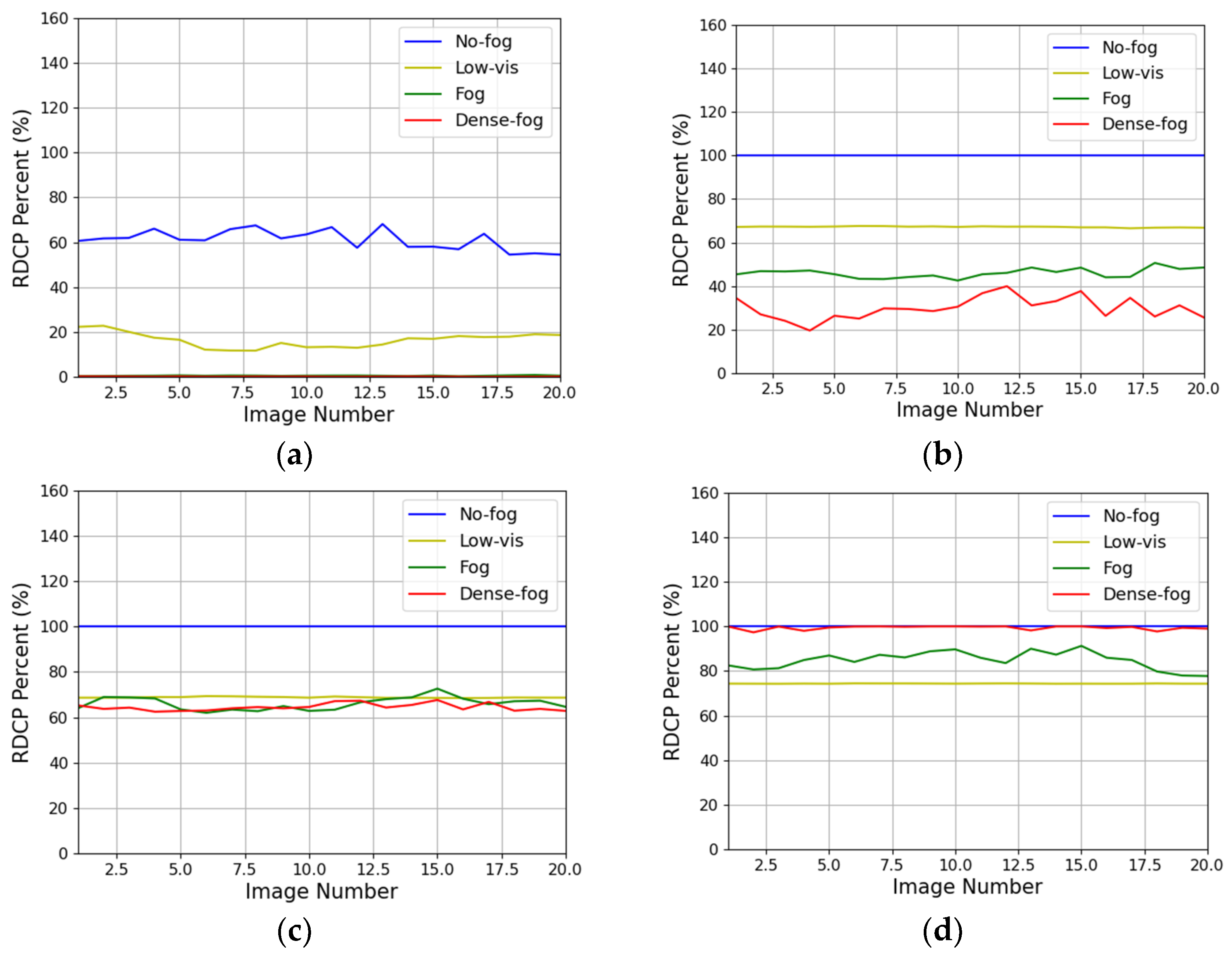
After applying the threshold, RDCP crops images in order to block out external light sources having similar DC values to sea fog.
Figure 12 shows the RDCP percentage value graphs of cropped images in different category labels. The value distinction in different categories becomes greater compared with
Figure 11. For example, no fog images have an average value of 62.3% in
Figure 11; however, the value dramatically increases to 95.6% in
Figure 12. Cropping the sky regions removes the ambiguity of DC values of an image, which means cropped images are less affected by external light sources. Therefore, the RDCP percentage values are more distinguishable by sea fog intensity and are sufficient to estimate the sea fog intensity from a single image. This implies that the height and shooting angle of the camera installation affects the accuracy of the RDCP algorithm. The recommended installation is that the sea part of an image must be more than 50% in a screen.
Optimization of the threshold is a critical factor for RDCP, as the performance of RDCP is highly affected by the value.
Figure 13 shows the changes in RDCP percentage values of 20 images captured from Ji Island when different thresholds are applied to the RDCP algorithm. The threshold values used here are 80, 110, 130, and 150, which are not the optimized value. Compared to
Figure 12d, the graphs fluctuate, which means that the sea fog intensity estimation is not stable in
Figure 13. Moreover, it can be seen that the RDCP values are not sufficient to play a role in sea fog intensity index. For example, when 80 is applied to the threshold, the graphs are overlapping with each other, since most DC values of the 20 images are greater than 80 regardless of sea fog intensity.
Another benefit of cropping is a reduction in complexity and calculation, which is helpful for energy saving.
Table 2 compares the average processing time and the number of pixels of 320 images for the RDCP value calculation. The sky region is removed so that the number of pixels for the RDCP value calculation decreases by up to 75%. The average processing time to estimate the fog intensity of 230 images is improved by up to 50% compared to the original image.
4.3. Visibility Estimation
The RDCP values and the visibility labels are discussed in this subsection. Using the RDCP percentage values, RDCP is able to estimate visibility in real-time. For this experiment, the RDCP algorithm is applied to real-time images from 6 a.m. to 6 p.m. at the Pyeongteak port on a day when sea fog changed significantly.
Figure 14 shows typical examples of sea fog images during the day. There was dense sea fog from 6 a.m. to 7:30 a.m., then the sea fog intensity gradually decreased, and finally the images showed a clear day.
The red graph in
Figure 15 indicates the visibility label values measured from a visibility meter on the same day. The visibility meter shows an error between 1100 h to 1500 h. The sea fog gradually disappears but rapidly became dense during the daytime, and dramatically disappears again. This is a typical error of visibility meters, which report dense fog while fog is actually gradually fading. However, RDCP utilizes the raw captured images, which contain the identical information as manual observation centers. The RDCP image processing results shows that fog gradually weakens from morning to evening.
Figure 15b demonstrates that RDCP is more reliable than visibility meters.
In
Figure 15a, the RDCP values of the original images are compared with the visibility label values in time and the RDCP values of the cropped images are compared in
Figure 15b. The RDCP values of cropped images reflect the real-time visibility changes better than the original images. For example, from 1500 h, the RDCP value of original images remains stable while the visibility label values continue to increase until 1700 h. This mismatch is caused since the original image is more influenced by external light sources from the sky region when the sky is very clear.
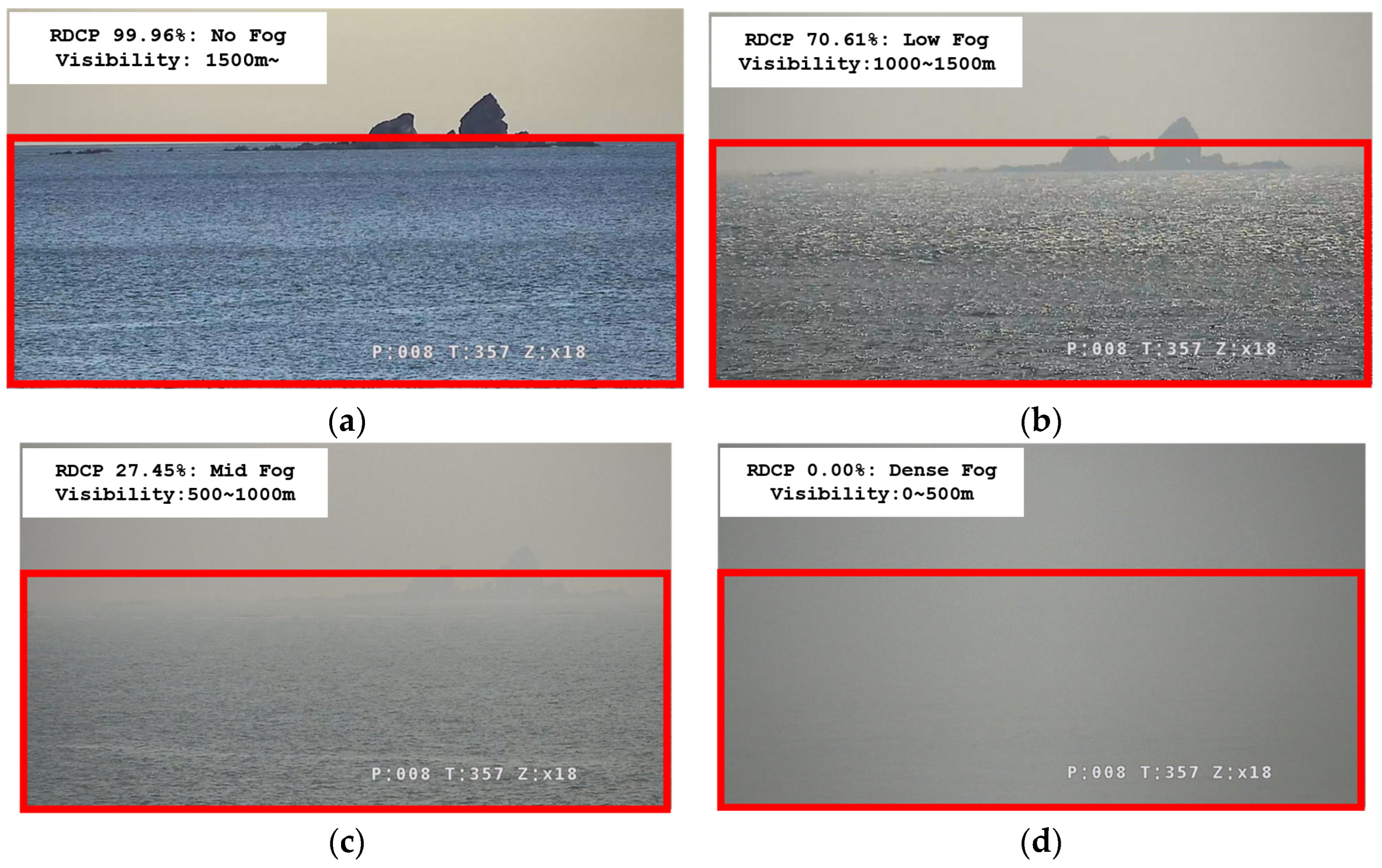
The prototype of RDCP is demonstrated using a camera at Baengnyeong Island port.
Figure 16 show results on different days and in different fog intensities. The information for sea fog intensity and visibility is displayed at the top left side of the screen. In
Figure 16, the RDCP percentage value matches the visibility labels described in
Table 1.
5. Conclusions
Visibility meters do not use visionary information, meaning that errors can occur, in particular in a sea environment. Therefore, this paper proposes the RDCP algorithm to estimate sea fog intensity and visibility by processing images captured from cameras which provide identical visional information as human eyes do. Moreover, RDCP estimates visibility at low cost for immediate use in many locations, on vessels, and on buoys. RDCP utilizes the dark channel acquiring process of the DCP algorithm, because the results of the acquiring process are sufficient to estimate fog intensity. Next, RDCP applies an optimized threshold to the acquired DC and then crops an image to exclude the sky region of the image. RDCP is a simple algorithm which does not require high computation; therefore, it is appropriate for ocean facilities, because of the usual battery operation.
320 raw images captured from cameras at the four ports in different locations and the labels along with those images are used for RDCP evaluation. Evaluation results show that the RDCP algorithm can provide more reliable fog intensity and visibility information than visibility meters. RDCP requires a single image for this estimation and, as a result, it shows good performance for real-time estimation, as the prototype of RDCP demonstrates. Therefore, it is expected that RDCP allows real-time and reliable fog density and visibility estimation at low cost and, consequently, the estimation is available in many marine activity points using the existing cameras installed, without any expensive additional equipment.
Author Contributions
Conceptualization, T.-H.I.; methodology, T.-H.I.; software, S.-H.H.; validation, S.-H.H. and T.-H.I.; formal analysis, T.-H.I.; investigation, S.-H.H.; resources, S.-H.H., S.-K.P. and K.-W.K.; data curation, S.-H.H.; writing original draft preparation, S.-H.H.; writing review and editing, S.-H.P.; visualization, S.-H.H.; supervision, S.-H.P.; project administration, T.-H.I.; funding acquisition, T.-H.I. All authors have read and agreed to the published version of the manuscript.
Funding
This research was supported by the Korea Research Institute of Ships and Ocean Engineering, and a grant from the Endowment Project Development of Open Platform Technologies for Smart Maritime Safety and Industries, funded by the Ministry of Oceans and Fisheries (1525014880, PES4880). This research was supported by the Korea Institute of Marine Science and Technology Promotion (KIMST) funded by the Ministry of Oceans and Fisheries, grant number 20210636. This research was supported by the Korea Institute of Marine Science and Technology Promotion (KIMST) funded by the Ministry of Oceans and Fisheries, grant number 201803842.
Institutional Review Board Statement
Not applicable.
Informed Consent Statement
Not applicable.
Data Availability Statement
Conflicts of Interest
The authors declare no conflict of interest.
References
- Korea Coast Guard. Available online: https://www.kcg.go.kr/kcg/na/ntt/selectNttInfo.do?nttSn=34010 (accessed on 20 October 2023).
- Shao, N.; Lu, C.; Jia, X.; Wang, Y.; Li, Y.; Yin, Y.; Zhu, B.; Zhao, T.; Liu, D.; Niu, S.; et al. Radiation fog properties in two consecutive events under polluted and clean conditions in the Yangtze River Delta, China: A simulation study. Atmos. Chem. Phys. 2023, 23, 9873–9890. [Google Scholar] [CrossRef]
- Wang, Y.; Lu, C.; Niu, S.; Lv, J.; Jia, X.; Xu, X.; Xue, Y.; Zhu, L.; Yan, S. Diverse dispersion effects and parameterization of relative dispersion in urban fog in eastern China. J. Geophys. Res. Atmos. 2023, 128, e2022JD037514. [Google Scholar] [CrossRef]
- Liang, C.W.; Chang, C.C.; Liang, J.J. The impacts of air quality and secondary organic aerosols formation on traffic accidents in heavy fog–haze weather. Heliyon 2023, 9, e14631. [Google Scholar] [CrossRef] [PubMed]
- Guide to Meteorological Instruments and Methods of Observation; World Meteorological Organization: Geneva, Switzerland, 2017; p. 1177.
- Korea Open MET Data Portal. Available online: https://data.kma.go.kr/climate/fog/selectFogChart.do?pgmNo=706 (accessed on 25 November 2023).
- Lee, H.K.; Shu, M.S. A Comparative Study on the Visibility Characteristics of Naked-Eye. Atmosphere 2018, 28, 69–83. [Google Scholar]
- The Korea Economic Daily: Ongjin County Council Urged the Ministry of Oceans and Fisheries to Ease the Visibility-Related Regulations. 18 October 2021. Available online: https://www.hankyung.com/society/article/202110280324Y (accessed on 25 November 2023).
- Xu, H.; Zhai, G.; Wu, X.; Yang, X. Generalized equalization model for image enhancement. IEEE Trans. Multimed. 2013, 16, 68–82. [Google Scholar] [CrossRef]
- Ma, Z.; Wen, J.; Zhang, C.; Liu, Q.; Yan, D. An effective fusion defogging approach for single sea fog image. Neurocomputing 2016, 173, 1257–1267. [Google Scholar] [CrossRef]
- He, K.; Sun, J.; Tang, X. Single image haze removal using dark channel prior. IEEE Trans. Pattern Anal. Mach. Intell. 2010, 33, 2341–2353. [Google Scholar] [PubMed]
- Wang, Y.K.; Fan, C.T. Single image defogging by multiscale depth fusion. IEEE Trans. Image Process. 2014, 23, 4826–4837. [Google Scholar] [CrossRef] [PubMed]
- Cai, B.; Xu, X.; Jia, K.; Qing, C.; Tao, D. Dehazenet: An end-to-end system for single image haze removal. IEEE Trans. Image Process. 2016, 25, 5187–5198. [Google Scholar] [CrossRef] [PubMed]
- Hu, H.M.; Guo, Q.; Zheng, J.; Wang, H.; Li, B. Single image defogging based on illumination decomposition for visual maritime surveillance. IEEE Trans. Image Process. 2019, 28, 2882–2897. [Google Scholar] [CrossRef] [PubMed]
- Xu, Y.; Wen, J.; Fei, L.; Zhang, Z. Review of video and image defogging algorithms and related studies on image restoration and enhancement. IEEE Access 2015, 4, 165–188. [Google Scholar] [CrossRef]
- Bae, T.W.; Han, J.H.; Kim, K.J.; Kim, Y.T. Coastal visibility distance estimation using dark channel prior and distance map under sea-fog: Korean peninsula case. Sensors 2019, 19, 4432. [Google Scholar] [CrossRef] [PubMed]
- Palvanov, A.; Cho, Y.I. Visnet: Deep convolutional neural networks for forecasting atmospheric visibility. Sensors 2019, 19, 1343. [Google Scholar] [CrossRef] [PubMed]
- Koschmieder, H. Theorie der horizontalen Sichtweite. In Beitrage zur Physik der Freien Atmosphare; Akademin-Verlag: Berlin, Germany, 1924; pp. 33–53. [Google Scholar]
- Huang, S.C.; Ye, J.H.; Chen, B.H. An advanced single-image visibility restoration algorithm for real-world hazy scenes. IEEE Trans. Ind. Electron. 2014, 62, 2962–2972. [Google Scholar] [CrossRef]
- Yang, L. Comprehensive Visibility Indicator Algorithm for Adaptable Speed Limit Control in Intelligent Transportation Systems. Ph.D. Thesis, University of Guelph, Guelph, ON, Canada, 2018. [Google Scholar]
- Jeon, H.S.; Park, S.H.; Im, T.H. Grid-Based Low Computation Image Processing Algorithm of Maritime Object Detection for Navigation Aids. Electronics 2023, 12, 2002. [Google Scholar] [CrossRef]
- Tarel, J.P.; Hautiere, N.; Caraffa, L.; Cord, A.; Halmaoui, H.; Gruyer, D. Vision enhancement in homogeneous and heterogeneous fog. IEEE Intell. Transp. Syst. Mag. 2012, 4, 6–20. [Google Scholar] [CrossRef]
- Sakaridis, C.; Dai, D.; Van, G.L. Semantic foggy scene understanding with synthetic data. Int. J. Comput. Vis. 2018, 126, 973–992. [Google Scholar] [CrossRef]
- Korea Meteorological Administration. Available online: https://www.kma.go.kr/neng/index.do (accessed on 20 October 2023).
- Korea Hydrographic and Oceanographic Agency. Available online: https://www.khoa.go.kr/eng/Main.do (accessed on 20 October 2023).
Figure 1.
Flow chart of the primary DCP processes.
Figure 1.
Flow chart of the primary DCP processes.
Figure 2.
Flow chart of the RDCP algorithm.
Figure 2.
Flow chart of the RDCP algorithm.
Figure 3.
DC value comparison of two sample images.
Figure 3.
DC value comparison of two sample images.
Figure 4.
The sample images used for
Figure 3. Both images are captured by an identical camera mounted in the same buoy. Image size is 1280 × 720 pixels. (
a) An image captured from the camera without sea fog; (
b) an image captured from the camera with dense sea fog.
Figure 4.
The sample images used for
Figure 3. Both images are captured by an identical camera mounted in the same buoy. Image size is 1280 × 720 pixels. (
a) An image captured from the camera without sea fog; (
b) an image captured from the camera with dense sea fog.
Figure 5.
Examples of cropped images from four different ports.
Figure 5.
Examples of cropped images from four different ports.
Figure 6.
Four different ports in which the datasets are captured in the Republic of Korea.
Figure 6.
Four different ports in which the datasets are captured in the Republic of Korea.
Figure 7.
Images captured at the Gwanghwa Island port and corresponding labels: (a) image having a no-fog label; (b) image having a low-fog label; (c) image having a mid-fog label; (d) image having a dense-fog label.
Figure 7.
Images captured at the Gwanghwa Island port and corresponding labels: (a) image having a no-fog label; (b) image having a low-fog label; (c) image having a mid-fog label; (d) image having a dense-fog label.
Figure 8.
Images captured at the Pyeongtaek port and corresponding labels: (a) image having a no-fog label; (b) image having a low-fog label; (c) image having a mid-fog label; (d) image having a dense-fog label.
Figure 8.
Images captured at the Pyeongtaek port and corresponding labels: (a) image having a no-fog label; (b) image having a low-fog label; (c) image having a mid-fog label; (d) image having a dense-fog label.
Figure 9.
Images captured at the Baengyeong Island port and corresponding labels: (a) image having a no-fog label; (b) image having a low-fog label; (c) image having a mid-fog label; (d) image having a dense-fog label.
Figure 9.
Images captured at the Baengyeong Island port and corresponding labels: (a) image having a no-fog label; (b) image having a low-fog label; (c) image having a mid-fog label; (d) image having a dense-fog label.
Figure 10.
Images captured at the Ji Island port and corresponding labels: (a) image having a no-fog label; (b) image having a low-fog label; (c) image having a mid-fog label; (d) image having a dense-fog label.
Figure 10.
Images captured at the Ji Island port and corresponding labels: (a) image having a no-fog label; (b) image having a low-fog label; (c) image having a mid-fog label; (d) image having a dense-fog label.
Figure 11.
RDCP percentage comparison of original images according to different sea fog intensity: (a) Gwanghwa Island; (b) Pyeongtaek (c) Baengyeong Island (d) Ji Island.
Figure 11.
RDCP percentage comparison of original images according to different sea fog intensity: (a) Gwanghwa Island; (b) Pyeongtaek (c) Baengyeong Island (d) Ji Island.
Figure 12.
RDCP percentage comparison of cropped images according to different sea fog intensity: (a) Gwanghwa Island; (b) Pyeongtaek (c) Baengyeong Island (d) Ji Island.
Figure 12.
RDCP percentage comparison of cropped images according to different sea fog intensity: (a) Gwanghwa Island; (b) Pyeongtaek (c) Baengyeong Island (d) Ji Island.
Figure 13.
RDCP percentage value changes according to the thresholds, showing 20 images captured at the Ji Island port: (a) when the threshold is 80; (b) when the threshold is 110; (c) when the threshold is 130; (d) when the threshold is 150.
Figure 13.
RDCP percentage value changes according to the thresholds, showing 20 images captured at the Ji Island port: (a) when the threshold is 80; (b) when the threshold is 110; (c) when the threshold is 130; (d) when the threshold is 150.
Figure 14.
Sea fog changes from the Pyeongteack port at different times of day.
Figure 14.
Sea fog changes from the Pyeongteack port at different times of day.
Figure 15.
Comparison of RDCP percentage (%) and visibility label value (km): (a) RDCP values of original images and visibility in km; (b) RDCP values of cropped images and visibility in km.
Figure 15.
Comparison of RDCP percentage (%) and visibility label value (km): (a) RDCP values of original images and visibility in km; (b) RDCP values of cropped images and visibility in km.
Figure 16.
Prototype of the RDCP algorithm was applied to a camera and real-time estimation was provided: (a) image with a no-fog label; (b) image with a low-fog label; (c) image with a mid-fog label; (d) image with dense-fog label.
Figure 16.
Prototype of the RDCP algorithm was applied to a camera and real-time estimation was provided: (a) image with a no-fog label; (b) image with a low-fog label; (c) image with a mid-fog label; (d) image with dense-fog label.
Table 1.
Label value comparison between sea fog intensity and visibility provided by KMAA and KHOA.
Table 1.
Label value comparison between sea fog intensity and visibility provided by KMAA and KHOA.
| Sea Fog Intensity | Visibility (m) |
|---|
| No-fog | 1500~ |
| Low-fog | 1000~1500 |
| Mid-fog | 500~1000 |
| Dense-fog | 0~500 |
Table 2.
Comparison of the average processing time and the related average number of pixels between 230 original images and 230 cropped images.
Table 2.
Comparison of the average processing time and the related average number of pixels between 230 original images and 230 cropped images.
| | Average Processing Time | Number of Pixels for the Algorithm Calculation |
|---|
| Original images | 34 ms | 921,600 |
| Cropped images | 17 ms | 329,707 |
| Disclaimer/Publisher’s Note: The statements, opinions and data contained in all publications are solely those of the individual author(s) and contributor(s) and not of MDPI and/or the editor(s). MDPI and/or the editor(s) disclaim responsibility for any injury to people or property resulting from any ideas, methods, instructions or products referred to in the content. |
© 2023 by the authors. Licensee MDPI, Basel, Switzerland. This article is an open access article distributed under the terms and conditions of the Creative Commons Attribution (CC BY) license (https://creativecommons.org/licenses/by/4.0/).


