Changes in Beaufort High and Their Impact on Sea Ice Motion in the Western Arctic during the Winters of 2001–2020s

Abstract

Sea ice affects the Earth’s energy balance and ocean circulation and is crucial to the global climate system. However, research on the decadal variations in the mean sea-level pressure patterns in recent winters (2001–2020) and the characteristics of sea ice motion (SIM) in the Western Arctic region is very limited. In this study, we utilized the Empirical Orthogonal Function (EOF) analysis method to investigate the potential impacts of Arctic Oscillation (AO) and Arctic Dipole (AD) on the Beaufort High (BH) during the period 2001–2020 and discuss the changes in SIM intensity in the Western Arctic. The results indicate that the negative phases of AO and AD are connected with (tend to bring about) a higher BH, strengthening anticyclonic circulation in the Arctic region. Conversely, the positive phases of AO and AD led to the collapse of the BH, resulting in a reversal of sea ice movement. Additionally, during the period 2001–2020, the BH consistently explained 67% of the sea ice motion (had the highest explanatory degree for sea ice advection within the region (weighted average 61.71%)). Meanwhile, the sea ice advection has become more sensitive to change in various atmospheric circulations. This study contributes to an in-depth understanding of the response of sea ice motion to atmospheric circulation in the Western Arctic in recent years, offering more explanations for the anomalous movement of sea ice in the Western Arctic.

1. Introduction

Sea ice is one of the most sensitive and important indicators of the marine environment and climate change. It plays an important role in regulating the exchange of materials and energy between the ocean and atmosphere [1]. In recent years, sea ice conditions in the Arctic have undergone notable changes, such as a decline in multiyear ice areas, thinning of the mean ice thickness, and acceleration of sea ice motion (SIM) [2,3,4,5]; these changes increase the sea ice cover’s sensitivity to atmospheric circulation [6,7,8]. In addition, the reduction in sea ice area is thought to play a dominant role in the “Arctic amplification” [9].

Arctic sea ice is affected by two atmospheric circulation systems during winter: the Eastern Arctic, which is primarily influenced by extratropical cyclones moving from Iceland along the North Atlantic storm path toward the Barents Sea [10,11]; and the Western Arctic, which is mainly influenced by a quasi-stationary high-pressure area known as the Beaufort High (BH) [12]. Notably, sea ice and ocean circulation in the Western Arctic is driven by this high-pressure system, and the associated anticyclonic winds largely control the mean circulation of Arctic sea ice [13]. In addition, the anticyclone-dominated Beaufort Gyre (BG) tends to transport sea ice away from the Canadian Archipelago westward into the Chukchi Sea (CS) [14]. However, when lower sea-level pressure (SLP) occurs across the Arctic Basin or when a persistent low-pressure system occurs in the southern Beaufort Sea (BS), it may cause a reversal of SIM in the Western Arctic [8,15].

The melting of sea ice has the potential to alter salinity and freshwater distribution in the ocean, thereby impacting ocean circulation and the formation of deep-water masses [16]. Furthermore, as the largest freshwater storage area in the Arctic Ocean [17], changes in sea ice circulation imply change in freshwater motion, affecting the Arctic Ocean salinity layer structure [18,19]. Therefore, the BG is important in regulating Arctic climate changes [20,21,22,23].

Arctic sea ice variability is primarily influenced by thermal and dynamic interactions between the atmosphere and ocean; sea ice dynamics are essential in the Arctic marine environment. For example, atmospheric circulation anomalies in winter can lead to the redistribution of sea ice and affect sea ice thickness in spring and sea ice extent in the summer [24,25]. The relationship between high-latitude Arctic atmospheric circulation, SIM, and sea ice extent has been well studied [26,27,28]. Moore et al. investigated the intensity and position of the BH in summer on decadal time scales and reported an increasing trend of the BH during summer from the late 1990s [29]. Petty et al. investigated seasonal trends and changes in ice circulation in the BG during the period 1980–2013; they reported that anticyclonic ice drift increased and responded to winds in all seasons in the late 2000s [30]. However, only a few studies have analyzed the interannual and interdecadal variability of the BH during recent winters (2001–2020) and ice motion in the region in response to BH variability. Therefore, we aim to reveal through this paper the potential impacts of the Arctic Oscillation (AO) and Arctic Dipole (AD) on the BH, and to conduct an in-depth investigation into the changes in sea ice advection in the Western Arctic Ocean and the decadal differences in its response to atmospheric circulation.

In the present study, we applied multi-source remote sensing data to analyze changes in the BH during the winters of 2001–2020 and their impact on the spatiotemporal motion of sea ice in the Western Arctic. Analyzing the variability in the extent of sea ice motion in the Western Arctic in response to dominant atmospheric modes can help elucidate the causes of abnormal sea ice motion within certain years. On this basis, the occurrence of natural disasters due to sea ice movement can be better predicted and avoided for the local economic and social development. Since the sea ice area in spring and summer is influenced by the sea ice movement during the previous winter, this study can help in the development and utilization of resources in the Arctic region and promote the sustainable development of the Arctic region.

2. Materials and Methods

2.1. Data

2.1.1. Sea Ice Drift

The SIM dataset used in this study is a reanalysis product of the National Snow and Ice Data Center (NSIDC). The product has a relatively high spatiotemporal resolution with the advantage of a long time series from October 1979 to December 2021. The NSIDC SIM product has better accuracy than other remote sensing-derived products [31,32]. This dataset contains daily and weekly SIM vectors and browsed images, representing weekly data. The remote sensing data source used by the product was derived from an Advanced Very High Resolution Radiometer (AVHRR), Advanced Microwave Scanning Radiometer—Earth (AMSR-E), Scanning Multi-channel Microwave Radiometer (SMMR), Special Sensor Microwave Imager (SSMI), Special Sensor Microwave Imager/Sounder (SSMI/S) sensors, International Arctic Buoy Programme (IABP) buoys, and the National Centers for Environmental Prediction/National Center for Atmospheric Research (NCEP/NCAR) reanalysis forecast for generating daily and weekly SIM estimates. The input SIM estimates were combined to produce a daily SIM product. To analyze the spatiotemporal variation in ice speed in the region and the variation in sea ice area flux between subareas, this study focused on daily ice speed vector data (Polar Pathfinder Daily 25 km EASE-Grid SIM vectors, Version 4). The data had a spatial resolution of 25 km and a temporal resolution of 1 day. Monthly and winter mean ice motion speed values were calculated by averaging the daily mean ice speed values.

2.1.2. Sea Ice Concentration

The sea ice concentration (SIC) data used to quantify sea ice area flux across flux gates in this study were obtained from the NSIDC. The dataset selected was the long time-series Bootstrap SIC from Nimbus-7 SMMR and DMSP SSM/I-SSMIS, Version 3. The dataset has a spatial resolution of 25 km and a temporal resolution of 1 day, spanning from November 1978 to May 2022. This SIC dataset was based on the measurement results of the Scanning Multichannel Microwave Radiometer (SMMR) on the Nimbus-7 satellite and the Special Sensor Microwave/Imager (SSM/I) sensors on the Defense Meteorological Satellite Program (DMSP) F8, F11, and F13 satellites. Additionally, it includes the measurement results from the Special Sensor Microwave Imager/Sounder (SSMIS) on the DMSP-F17. The SIC for this dataset was derived from a modified bootstrap algorithm that uses a dynamically adjusted set of sea ice and seawater tether points. A detailed analysis of two passive microwave algorithms for SIC, the bootstrap algorithm, and the NASA team algorithm was presented by Comiso et al.; please refer to the studies on passive microwave algorithms for SIC [33].

2.1.3. Sea Ice Age

To determine whether spatiotemporal variations in sea ice motion speed are related to multiyear ice distribution, the sea ice age data used in this study were taken from the NSIDC dataset (EASE-Grid Sea Ice Age, Version 4). Common information about this dataset is shown in

Table 1. Summary of all data sets engaged during this study.

Data Category	Data Source	Sensors	Temporal Coverage	Spatial Resolution	Temporal Resolution
Ice Motion	NSIDC	AMSR-E, AVHRR, DRIFTING BUOYS, SMMR, SSM/I, SSMIS	October 1978–December 2021	25 km × 25 km	daily
Ice Concentration	NSIDC	SMMR, SSM/I, SSMIS	October 1978–May 2022	25 km × 25 km	daily
Ice Age	NSIDC	AMSR-E, AVHRR, DRIFTING BUOYS, SMMR, SSM/I, SSMIS	January 1984–December 2021	12.5 km × 12.5 km	weekly
Sea-Level Pressure	ECMWF	-	1959–present	0.25° × 0.25°	monthly

. The SIM vector data used to create this dataset are derived from the weekly Polar Pathfinder Daily 25 km EASE-Grid SIM vectors, Version 4; they are bilinearly interpolated to a 12.5 km × 12.5 km EASE-Grid. This method estimates the age of sea ice by considering each grid cell containing ice as a discrete and independent Lagrange package, and tracking the packages driven by weekly ice motion in a weekly time step.

2.1.4. Atmospheric Data

To calculate the atmospheric circulation indices used in this study, SLP data at a single level from the ERA5 dataset of the European Center for Medium-Range Weather Forecasts (ECMWF) with a horizontal resolution of 0.25° × 0.25° were used. ERA5 is the fifth generation of climate reanalysis datasets released by the ECMWF and the successor of the ERA-I dataset; its advantages over the ERA-I dataset are improved availability and higher temporal resolution (per hour) [34]. The ERA5 dataset provides a wide range of atmospheric and surface parameters from 1950 to date, using the assimilation scheme of 4-Dimensional Variation Analysis (4D-Var) of the Integrated Forecast System (IFS) with a vertical resolution of 137 layers (mixed layer) and a mode top layer of 0.01 hPa.

2.2. Methods

2.2.1. Empirical Orthogonal Function

Empirical orthogonal function (EOF) analysis was first proposed by Pearson in 1902 and introduced by Lorenz in the 1950s in meteorological and climatic studies for application to relevant problems in analyzing multivariate data in meteorology [35]. It has become a common spatiotemporal analysis method in atmospheric science that can transform a complex 3D spatiotemporal dataset into a linear combination of multiple spatial modes and their corresponding time series, simplifying the original dataset by reshaping most of the variance interpretation of the original data to a few modes and reducing many physical processes dominant in space and time [36].

We split the field of the mean sea-level pressure (MSLP) in winter ($X_{m\times n}$) over the two interdecadal periods into two components—as functions of time and space:

$$X_{m\times n}=V_{m\times p}\times T_{p\times n}$$

(1)

where V is the spatial eigenvector, T is the time factor, m is the grid point, and n is the time-series length.

Observation x_ij for any spatial location point i at time point j can be viewed as a linear combination of p spatial functions v_ik, and temporal functions t_kj:

$$x_{ij}={\sum }_{k=1}^p{v}_{\mathit{ik}}{t}_{\mathit{kj}}=v_{i1}{t}_{1j}+v_{i2}{t}_{2j}+\dots +v_{\mathit{ip}}{t}_{\mathit{pj}}$$

(2)

The original data matrix $X_{m\times n}$ is first transformed into a square matrix $Y_{m\times m}$ when performing EOF analysis.

$$Y_{m\times m}=\frac{1}{n}X\times X^T$$

(3)

Then, the eigenroots λ and eigenvectors $V_{m\times m}$ of the square matrix Y are calculated:

$$Y_{m\times m}\times V_{m\times m}=V_{m\times m}\times {\Lambda }_{m\times m}$$

(4)

where ${\Lambda }_{m\times m}$ is a diagonal matrix consisting of eigenvalues ${\lambda }_i$ arranged from the largest to the smallest. Any non-zero eigenroot ${\lambda }_i$ will correspond to a column of eigenvector values called the ith spatial mode of the original data. Different columns of the eigenvector $V_{m\times m}$ correspond to different spatial modes of the EOF:

$${\mathit{EOF}}_i=V(:,i)$$

(5)

The time coefficients corresponding to the spatial eigenvectors are obtained by projecting the calculated eigenvectors onto the original data matrix X:

$$P{C}_{m\times n}=V_{m\times n}^T\times X_{m\times n}$$

(6)

where each row of data in PC is the time coefficient corresponding to each eigenvector; for example, PC(1,:) is the time coefficient corresponding to the first spatial mode.

In addition, the variance contribution ${\mathsf{\rho }}_i$ of the ith spatial mode to the original data field is

$${\rho }_i={\lambda }_i/{\sum }_{i=1}^m{\lambda }_i$$

(7)

2.2.2. Atmospheric Circulation Indices

The BH, typically located in the BS area of the Arctic Ocean, may slightly vary in its precise location with seasonal and interannual changes. Then, in our study, similar to researchers like Moore et al., the BH is regarded as a quasi-stationary high-pressure system [8] and is important for regulating the BG, SIM, and material balance in the BS. The strength of the BH was measured by calculating the MSLP in the range 75° N–85° N, 170° W–150° E using ERA5 reanalysis data. In addition, to determine whether there are significant interdecadal differences in the BH and SIM in the Western Arctic, we defined the periods 2001–2010 and 2011–2020 as the D1 and D2 interdecadal periods, respectively.

The Central Arctic Index (CAI) is the difference in SLP between 84° N, 90° W and 84° N, 90° E (shown as red pentagrams in Figure 1), and it can be used to explain the meridional motion of sea ice [37]. In this study, the CAI was calculated using a reanalysis of the monthly MSLP data from ERA5.

$$I_{\mathit{CAI}}={\mathit{SLP}}_{84°N90°W}-{\mathit{SLP}}_{84°N90°E}$$

(8)

The AO and AD index is the time coefficient of the first two modes of the EOF analysis of the monthly MSLP north of 70° N [38,39]. In this study, the AO and AD index was obtained via EOF analysis using monthly MSLP reanalysis data north of 70° N for ERA5 from 2001 to 2020.

2.2.3. Estimation of Area Flux and Error Analysis

The sea ice area flux is the area of sea ice that passes through a specific flux gate within a specified time, quantifying the strength of the SIM in the region. In this study, we predetermined two latitudinal flux gates, A1 and A2, and two meridional flux gates, B1 and B2, to estimate the sea ice area flux. However, each flux gate was used to divide the study region into three subareas, namely BS, CS, and the North Western Sector of the Arctic (NWSA), as shown in Figure 1. The arrangement of flux gates was modified and slightly increased, compared to that in a previous study [30], to include the different study objectives and to better estimate sea ice transport between the subareas in the study region. We resampled at approximately 25 km intervals along the flux gate track using daily sea ice drift data and SIC data provided by the NSIDC. The sea ice area flux F was calculated from the data at each sampling point using the following equation:

$$F={\sum }_{i=1}^{N-1}{u}_i{C}_i∆x(i=1,2,\dots ,N)$$

(9)

where $u_i$ is the component of motion perpendicular to the flux gates at each sampling point, $C_i$ is the SIC obtained by resampling at each point, and $∆x$ is the sampling interval along the gate (~25 km). The daily sea ice transport at each flux gate was aggregated to obtain the area of sea ice passing through each flux gate during the winter.

To calculate the area flux, the area flux errors for each flux gate were quantified by applying the uncertainty equation in the flux estimation for each flux gate, assuming that the sea-ice drift speed errors at each sampling point on the flux gates were independent, unbiased, and normally distributed [40]:

$${\delta }_F=\frac{{\delta }_e}{\sqrt{N_s}}L$$

(10)

where ${\delta }_e$ is the assumed error in the sea-ice drift speed in the study region during the freezing period (~1.69 km/d), L is the flux gates’ length (km), and Ns is the number of sampling points on the flux gates’ tracks. ${\delta }_e$ was determined based on buoy data from the NSIDC/Pathfinder product and the IABP, which were systematically assessed and compared [31].

3. Results

3.1. Changes in BH and other Atmospheric Circulation Patterns in Winters of 2001–2020

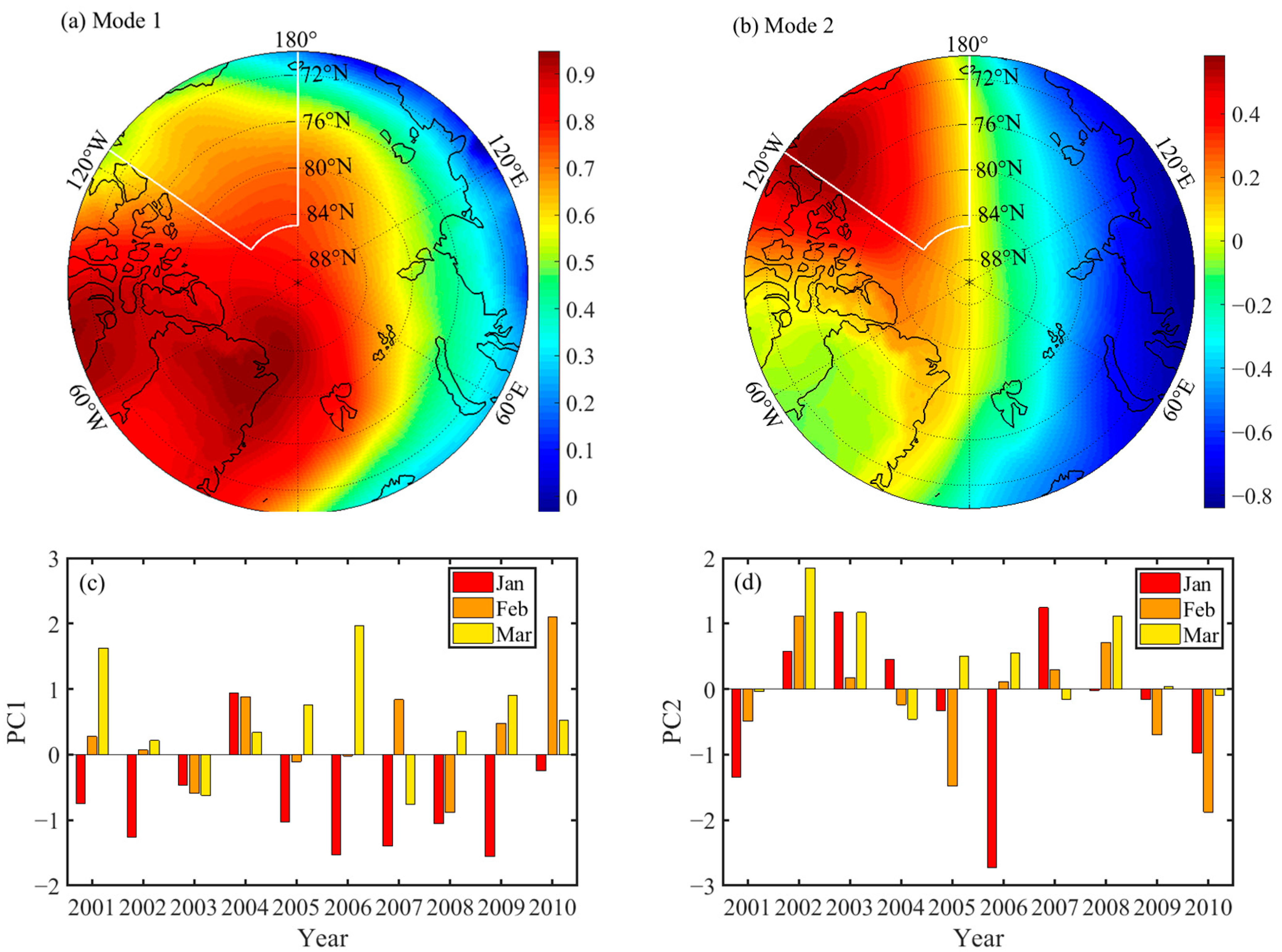
3.1.1. Interannual Variability in Atmospheric Patterns

Figure 2 presents the BH time series calculated from the ERA5 reanalysis of the SLP data during the winters of 1979–2020 (January, February, and March). The results show that the BH has significant interannual and trend variability, with the highest and lowest BH occurring in the winters of 2013 and 2017, respectively (1033.43 hPa and 1010.03 hPa). In addition, the BH time series shown in Figure 2 indicates trend variability, with a significant upward trend in the BH during the winters of 1989–2000 and a slow downward trend at the 95% significance level during the winters of 2001–2020. In both intervals, frequent intrusions of the North Atlantic low-pressure system in the winters of 2017/2020 resulted in a stronger downward trend and lower mean BH in D2 than in D1 (~3.1 hPa) [8,15].

Although the BH dominates sea ice motion in the Western Arctic [12], the AO and the AD patterns are also important for the Arctic sea ice motion. The positive phase of the AO (+AO) reduces winter ice thickness and influences the basin-scale anticyclonic sea ice drift [41]. When the AO is in an extreme high positive phase, sea ice in the Arctic region even exhibits cyclonic circulation [26]. Since the AD shows a strong meridionality, the positive phase of the AD (+AD) leads to an acceleration of the transpolar sea ice drift, facilitating the export of sea ice from the Arctic Basin, whereas the negative phase of the AD (-AD) often accompanies a stronger Beaufort Gyre, which is conducive to the accumulation of sea ice and freshwater in the Arctic Basin, directly leading to a reduction in the export of sea ice from the Arctic Basin [39].

So, winter-averaged AO and AD indices and the CAI were calculated to determine the extent to which these atmospheric patterns influence sea ice motion in the region (Figure 3). The results show that all three have large interannual variability over the 2001–2020 period but do not show a trend as significant as that for the BH, except for the significant upward trend of AD in the past decade.

3.1.2. Interdecadal Differences of SLP in the Arctic

Before performing EOF analysis on the sea-level pressure data, the data were preprocessed. This included subtracting the climatological average from the original data at each time point. Next, a linear regression analysis was performed on the data after removing the average to identify any existing linear trends. Then, this linear trend was subtracted from each data point to ensure that the data did not contain seasonal or other cyclical variations. Finally, the dominant pattern of MSLP north of 70° N over two interdecadal periods and the corresponding time coefficients were analyzed using EOF (Figure 4 and Figure 5).

Figure 4a and Figure 5a show the negative phase of the AO (−AO), while Figure 4b and Figure 5b show the +AD. However, the positive and negative phases within specific years should be determined in conjunction with the corresponding time coefficients (the positive, negative, and magnitude of the time series indicating the tendency of the corresponding EOF mode to occur at a given point in time).

The variance contribution rates of the first mode during the D1 and D2 are 51.97% and 53.48%, respectively, while those of the second mode are 18.46% and 20.18%, respectively. The cumulative variance contribution rates of the first two modes both exceed 70%. Therefore, we only consider the spatial differences of the first two modes. The results show that during the winters of 2001–2020, the main modes of MSLP in the Arctic region maintained a certain consistency. Both the first and second modes exhibit features similar to the AO and the AD (Figure 4 and Figure 5). However, the years with extremely strong AO and AD increased, and the pressure anomaly center of the first mode became stronger and moved toward the Arctic center within the D2. This has led to extremely strong +AO (2020) or −AO (2013) in the last decade, potentially resulting in strong anticyclonic sea ice circulation or a reversal of sea ice motion. Meanwhile, in the second mode, the pressure anomaly center on the west side of the Arctic moved toward Greenland. This change may cause a stronger east–west pressure gradient, thus accelerating or slowing down the transpolar flow of sea ice.

3.2. Spatiotemporal Variability of Sea Ice Motion Velocities

3.2.1. Long-term Variability in Sea Ice Motion Velocities

As shown in Figure 6d, the speed of the Arctic sea ice drift indicated a statistically significant positive trend (p < 0.001) during the slow decline in the BH during the winters of 2001–2020.

The increase in the sea ice drift speed was the highest in March (0.115 km/d, Figure 6c) and the lowest in January (0.084 km/d, Figure 6a). The increase in SIM speed in winter across the study region was 0.095 km/d (Figure 6d), which was 23.38% higher than the climatic mean value (winters 1979–2020, 0.077 km/d). Notably, the rate of sea ice growth was comparable in January and February; however, ice growth was significantly higher in March than in January and February. In addition, the mean ice velocities in January, February, and March within the D1 were 5.27 km/d, 5.18 km/d, and 3.96 km/d, respectively. Contemporaneous ice velocities within the D2 were 6.58 km/d, 5.67 km/d, and 4.86 km/d, respectively. The fastest increase in average ice speed was recorded in January (24.98%). This may have been due to the progressively increasing melting period in the Arctic (~20 days); that is, early melting and late freezing [42]. Combined with the decrease in the average sea ice thickness in the Arctic, the interaction forces within the sea ice have weakened and may be more susceptible to atmospheric forcing.

The results obtained in this study differ from those of previous studies with respect to the period covered and the data products used. The calculated winter ice speed increase was greater than that estimated from December to May in a previous study (0.06 km/d) [4]. Although trends in ice drift velocities obtained from different data sources may differ in magnitude, all results indicate an increasing trend in ice speed.

3.2.2. Spatial Variation of Sea Ice Drift Speed

Long-term trends in sea ice drift velocities in the three subareas indicated significant spatial heterogeneity during the winters of 2001–2020. As shown in Figure 7a, the positive trends in the drift speed for the BS (0.096 km/d, p < 0.05), CS (0.095 km/d, p < 0.05), and NWSA (0.092 km/d, p < 0.01) were generally commensurate and greater than the mean ice-drift speed growth trend across the study region (0.095 km/d, p < 0.01). Positive trends in the BS and NWSA increased in the three subareas within D1 and D2 relative to the growth trend in the 1979–2020 winters.

To be able to represent the mean ice speed or ice speed anomalies in the subarea more visually, the mean sea ice speed and mean ice speed anomalies for each subarea during D1 and D2 are listed in

Table 2. Mean ice speed and ice speed anomalies of subareas in the Western Arctic.

Subarea	Mean Ice Speed (km/d)		Ice Speed Anomaly (km/d)
	D1	D2	D1	D2
BS	4.97 ± 0.67	6.02 ± 1.35	0.29	0.88
CS	6.59 ± 0.5	7.58 ± 1.27	0.44	0.79
NWSA	4.92 ± 0.83	5.80 ± 0.84	0.21	0.60

Note: The ice speed anomaly value is the mean ice speed in D1 and D2 compared with the climatic mean value (winters 1979–2020).

. The increase in mean ice speed was most significant in the BS (21.18%), followed by the NWSA (17.89%) and CS (15.07%), and the mean ice speed anomalies in the three subareas were 0.29 km/d, 0.44 km/d, and 0.21 km/d within the D1, respectively. Generally, the mean ice speed anomalies were low in the study region (especially in the NWSA), with higher positive speed anomalies only in the southernmost part of the study region, as shown in Figure 7b. In addition, this may have further increased sea ice mobility and deformation as Arctic sea ice thickness and SIC decreased continuously [3,6], facilitated by the extreme Arctic cyclones, which have been more common in recent winters [43]. As a result, the mean ice speed anomalies in the BS, CS, and NWSA have increased to 0.88 km/d, 0.79 km/d, and 0.59 km/d, respectively. Regarding spatial distribution, the regions with high positive ice speed anomalies within D2 were mainly located south of the BS and central CS. Conversely, the positive anomalies in the NWSA were generally low (Figure 7c). In addition, by comparing the mean speed anomalies between the two interdecadal periods, it can be seen that within D1, a higher value of the mean positive ice speed anomaly was observed in the CS; however, the increase in the mean ice speed anomaly was apparent in the BS and NWSA within D2 (Table 2).

A previous study demonstrated that changes in the Arctic sea ice thickness during winter are the primary determinants of ice speed variability [44]. Similarly, we argue that spatiotemporal variability in Western Arctic sea ice speed on an interdecadal scale during the 2001–2020 winters was related to changes in the multiyear ice area and sea ice thickness. Within D1, multiyear ice (thick ice) was spread throughout the Western Arctic, and a significant proportion (59.43%) of this multiyear ice was >5 years of age (Figure 8a). However, the area of multiyear ice >2 years has decreased by 42.92% in the last decade relative to D1, and the area of sea ice with 4 years of age has decreased by 86.19%. During this time, multiyear ice older than 3 years dominated and gradually retreated toward the Northern Canadian Arctic Archipelago (Figure 8b). As older sea ice in the Arctic melts, sea ice thickness and internal ice stress decrease, and the impact of the increased cyclonic activity on SIM becomes apparent, as observed in the winter of 2013 with a strong anticyclonic circulation in the Western Arctic, and in the winters of 2017 and 2020 with a reversal of SIM in the Western Arctic due to increased storm activity [8,15].

3.3. Sea Ice Motion Changes in the Western Arctic

Sea ice transport caused by the SIM regulates the Arctic sea ice material balance. As a circulation system regulating Arctic sea ice drift, the strength of the BG affects regional multiyear ice motion, freshwater transport, sea ice circulation, the material balance between Arctic seas, and the export of Arctic sea ice to lower latitudes [21,30,44]. Therefore, one of the focuses of this study is to analyze the recent changes in ice circulation between subareas in the Western Arctic, determine whether they are related to changes in BH, and quantify them by calculating the area flux at each flux gate.

Details of the four flux gate arrangements and the results of the area flux errors calculated according to Equation (9) are presented in

Table 3. Sea ice area flux error estimates.

Fluxgates	Location	L (km)	Ns	σwinter (km2/d) (Jan–Mar)
A1	BS–NWSA	572.86	24	197.62
A2	CS–NWSA	479	20	181.01
B1	BS–CS	889.56	37	247.15
B2	CS–East Siberia Sea	889.56	37	247.15

Note: L denotes flux gate length, Ns is the number of sampling points on the flux gates, and σ_winter denotes flux errors.

, where the calculated positive (negative) area flux of sea ice indicates the outflow (inflow) of sea ice for the former sea area.

3.3.1. Variation in Sea Ice Area Flux between Subareas

Figure 9 shows the estimates of sea ice area flux through the four flux gates using the NSIDC/Pathfinder sea ice drift product and SIC data from the NSIDC. A strong agreement (R² = 0.86, p < 0.001) was observed in the area flux between the two meridional flux gates (B1 and B2) during the winters of 2001–2020. Within D1, the interannual variability in the area flux in B1 and B2 was small. In contrast, within D2, a higher agreement was observed between the two fluxgates (R² = 0.90, p < 0.001) owing to frequent crucial changes in the BH, resulting in significant fluctuations in sea ice transport in the Western Arctic (with a larger standard deviation) and indicating that sea ice flows out of the BS in winter; in addition to the loss in the CS, part of the sea ice flows through B2 to the East Siberian Sea (or reverse flow).

Figure 9 shows the interannual variability in sea ice transport between subareas within the study region; when the area flux exceeds the gray shading, an extreme sea ice exchange has occurred. A1 represents the primary threshold at which sea ice from the NWSA enters the BS. The mean area flux through the fluxgate during the winters of 2001–2020 was −4.75 ± 1.78 × 10⁴ km², indicating the dominance of sea ice inflow. As shown in Figure 9a, the maximum values of sea ice inflow and outflow were in 2013 and 2019, respectively. The influence of the collapse of the BH would lead to a reversal of sea ice in the Western Arctic during the winters of 2017 and 2020 [8,15], resulting in a major change from the inflow to an outflow of sea ice in the BS. At the A2, the mean winter area fluxes in D1 and D2 were 2.22 ± 1.63 × 10⁴ km² and 4.90 ± 1.63 × 10⁴ km², respectively, with the latter more than twofold the former, suggesting that the slow decline with BH leads to an increase in the area of sea ice inflow from the CS to the NWSA. The mean sea ice area flux for B1 and B2 in winter within the D1 was −1.15 ± 0.22 × 10⁵ km² and −6.91 ± 2.22 × 10⁴ km², respectively; they reached maximum sea ice outflow area in winter 2013, −4.85 × 10⁵ km² and −3.94 × 10⁵ km², respectively, and maximum sea ice inflow area in winter 2017, 2.11 × 10⁵ km² and 3.27 × 10⁵ km², respectively. The results show that in some years, when extreme BH events occurred, extreme sea ice movements between regions also occurred, such as those in 2013 and 2017.

However, according to our predictions, with the recent weakening of the BH, interregional SIM will weaken. In addition, the sea ice flowing out of the BS through B1 was much greater than that in the other seas (

Table 4. Mean annual area flux and trends for each flux gate within different interdecadal periods.

Fluxgates	Mean Ice Area Flux (km2/a)		Trend (km2/a)
	D1	D2	D1	D2
A1	−43,874.90	−51,093.85	5213.79	13,128.3
A2	22,187.71	48,953.16	5315.22	12,637.8
B1	−112,430.87	−117,086.61	393.3	12,730.5
B2	−55,552.21	−82,669.55	10,035.9	14,346.9

Note: A significant trend change was observed in the area flux only at A2 within D2.

). Therefore, sea ice area loss in the BS can largely explain the total annual sea ice area loss, consistent with the findings of previous studies [45,46,47].

Furthermore, with the emergence of meridional winds derived from the +AD mode, the meridional flow of sea ice is accelerated [48]; the rapid drift of sea ice recorded at the MOSAiC observatory was also caused by the persistent +AO and +AD [49]. Consequently, during the D2 period, the frequent occurrence of +AO and +AD together (2011/2017/2019/2020, Figure 5c,d) accelerated the meridional flow of sea ice, leading to extreme values of sea ice advection at locations A1 and A2 in the corresponding years (Figure 9a,b) and an increasing trend in area flux (Table 4).

The mean area flux through each flux gate increases within D2 (Table 4); we suggest that this is related to the stronger BH in the winters of 2013, 2016, and 2018 (Figure 2). The stronger anticyclonic circulation in the Western Arctic, influenced by the BH during these three years, accelerated the interregional SIM, increasing the mean sea ice area flux within D2.

Regarding trend variability, there were clear interdecadal differences in sea ice transport within the region. For the two latitudinal flux gates, A1 and A2, the trends varied similarly over the same period and were more positive over D2; however, considering the two meridional flux gates, B1 did not show a significant trend in area flux variability over D1, with an abrupt increase in trend over D2, while B2 showed relatively little trend variability over the two interdecadal periods (Table 4). This suggests that as the BH slowly declined within D1 and D2, the trend of SIM between subareas in the Western Arctic diminished in parallel. In contrast, as the decreasing trend of the BH increased, the decrease in sea ice transport between the subareas showed a more positive trend.

3.3.2. Response of Sea Ice Motion to Atmospheric Circulations

To investigate the extent to which sea ice transport in the Western Arctic responded to several atmospheric circulations, including the BH, during the 20 years of the slow decline in the BH, we calculated the coefficient of determination (R²) between the area flux and atmospheric circulation indices for each flux gate, as shown in

Table 5. Determination coefficients of atmospheric circulation indices and sea ice transport in the winters of 2001–2020.

Atmospheric Circulation Indices	A1	A2	B1	B2
BH	0.76 ***	0.42 **	0.64 ***	0.53 ***
CAI	0.55 ***	0.51 ***	0.36 **	0.32 **
AO	0.39 **	0.44 **	0.33 **	0.18 **
AD	0.23 *	n.s.	n.s.	n.s.

Note: Significance levels are p < 0.001 (***), p < 0.01 (**), and p < 0.05 (*); n.s. denotes non-significance at the 0.05 level.

.

In the winters of 2001–2020, for the same flux gate (other than A2), BH explained the highest degree of SIM in the study region among several atmospheric circulation models. For example, for A1, the variation in BH explained 76% of the variation in sea ice area from the BS to the NWSA (p < 0.001). In addition, because the AO index measures non-seasonal changes in the SLP north of 20° N, it is less explanatory of the local SIM in the Arctic. Therefore, the AO is less explanatory of the same intersea ice motion than the CAI and BH (Table 5). Due to the unusually strong meridional nature of AD, it is an important mechanism driving Arctic sea ice and cold air into the Barents Sea, Nordic Seas, and Northern Europe, and can adequately explain the sea ice export from the Fram Strait [40]. Therefore, the changes in AD can explain the 32% and 56% changes in sea ice advection at A1 and A2, respectively. The reason for the large difference in the degree of explanation may be due to the more distinctive spatial distribution of AD within D2. Notably, the BH acts as a high-pressure system prevalent in the Western Arctic Ocean region during winter. Although it profoundly affects SIM in the Western Arctic, for SIM at the A2, the CAI has a higher degree of variability in area flux than the BH, at 51% and 42%, respectively. This is primarily because the CAI can better depict the sea ice movement in the central region of the Arctic Ocean [32].

Regarding the interdecadal variability in the response between sea ice motion and atmospheric circulation, the BH and CAI only significantly affected the SIM at the two latitudinal flux gates (A1 and A2) during D1. The BH explained 89% of the variation in area flux at A1 (p < 0.001), which is the highest degree. During the same period, AO and AD were significantly correlated with the area flux at A2 (R² = 0.51 and R² = 0.47, respectively). There wasa a large interannual variability in sea ice transport between subareas in winter during D1 (Figure 9); therefore, to investigate whether this fluctuation is related to the downward trend in the BH, we calculated the correlation between the two to quantify the magnitude of the effect (Figure 10a–d). A significant negative correlation existed between the BH and the area flux of each flux gate. The coefficients of determination between the ice area flux at A1, B1, and B2 were relatively high (0.86, 0.88, and 0.73, respectively). Conversely, the interpretation of sea ice flow between the CS and NWSA was low (Figure 10b, R² = 0.47, p < 0.05); this may be related to the circulation of sea ice in the Western Arctic due to the annular character of the high-pressure region. For example, BG in the Western Arctic is stronger when extremely high pressures are present. However, A2 is located near the center of the circulation zone, where the meridional ice speed is low. Ice speed is the dominant factor in winter influencing area flux; thus, the area flux at A2 is less responsive to BH. In contrast to the negative correlation between BH and sea ice transport, AO and CAI generally showed a significant positive correlation with sea ice transport between subareas. SIM in the Western Arctic responds to the two atmospheric modes to a comparable extent, with coefficients of determination within 0.49–0.66 (Figure 10i–p).

Our findings indicate that the trend in sea ice transport in the study region has weakened with the weakening of the BH over the last 20 years. Simultaneously, the extent to which various types of atmospheric circulation explained SIM was generally enhanced within the D2 compared to the D1. For example, there was no significant relationship among the BH, CAI, AO, and the area flux at the two meridional flux gates (B1 and B2) within D1. However, the extent to which these types of atmospheric circulation explained the area fluxes was enhanced within D2. This may be due to the reduction in sea ice thickness and multiyear ice area in recent years (Figure 8), which has led to a weakening of the internal ice forcing, combined with the enhancement of the meridional flow of sea ice in recent years [48,49], which has made it more susceptible to various atmospheric forcings.

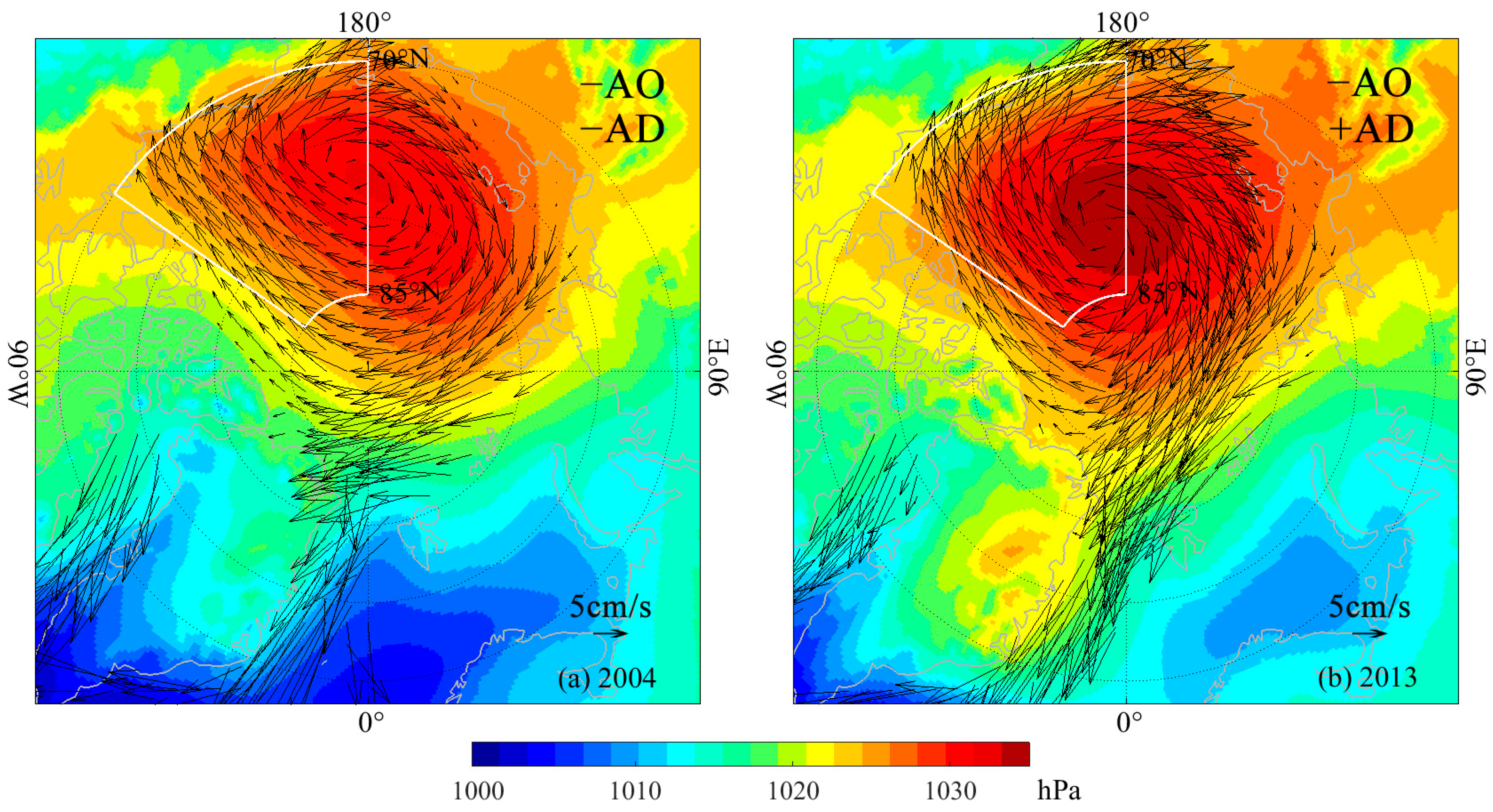
4. Discussion: Sea Ice Motion under Different BH Conditions

In this study, we used satellite remote sensing data to analyze the variability in BH and the spatiotemporal variability in SIM in the Western Arctic during the winters (JFM) of 2001–2020. However, our study differed from Kuang et al. by considering systematic errors in the estimation of area flux caused by different SIM and SIC data sources [50], focusing more on estimating the interannual and interdecadal trend variabilities of sea ice area flux through each flux gate and analyzing the response of area flux to atmospheric circulation. As the thinning of the Arctic sea ice continues to occur, more frequent pan-Arctic intrusions of the North Atlantic low-pressure system may have implications for the BH and climate of the region [8]. In addition, given the role of the BH in sea ice transport, its extremes significantly impact sea ice transport within the study region. In recent years, the BH has exhibited large interannual variability, and it is unclear whether the weakening of the BH in winter and the large interannual variability will persist. To understand the differences in sea ice motion within the study area under different BH conditions, we used a threshold of 1.5 standard deviations below/above the climate mean (winters of 1979–2020) to measure the years with extreme low/high BH in the winters of 2001–2020 and a threshold of ±0.5 standard deviations to define the normal BH case.

In recent years, with the intensification of the Arctic amplification effect, the thickness of Arctic sea ice has gradually decreased, resulting in greater mobility of the sea ice. Therefore, under different SLP patterns, the characteristics of SIM have become more distinctly different. It is important to note that there can be differences in SIM patterns with the same BH index. This is because the BH index is calculated as the MSLP for a given area, and the central location and strength of the BH affect SIM [51]. Figure 11a,b show the MSLP and SIM patterns in winter during extremely high pressures in the study region. As the dominant mode, when the AO is in a negative phase, the MSLP in the Arctic region is relatively high, and clockwise sea ice movement almost controls the entire Arctic Ocean. Moreover, with the intensification of the −AO in 2013, there is a more pronounced high-pressure anomaly center in the Arctic region, resulting in stronger anticyclonic circulation in the area. In addition to the significant impact of AO on sea ice movement, different phases of the AD also affect the flow of Arctic sea ice. For instance, the +AD in 2013 would lead to more sea ice flowing out of the Arctic through the Fram Strait (Figure 11b). Therefore, the loss of sea ice in the Arctic region and the patterns of sea ice movement within the region may be jointly determined by AO and AD.

When the AO is in its positive phase, the BH is at a lower level, and the North Atlantic low-pressure system extends northward through the Barents Sea, leading to the gradual dominance of low-pressure systems in the Arctic Ocean (Figure 12). Unlike the anticyclonic sea ice circulation in the Arctic under −AO conditions, the lower BH combined with +AO in 2017 and 2020 caused varying degrees of reversal in sea ice movement. In 2020, with a stronger +AO and +AD, the central pressure of the low-pressure system was lower and its coverage was broader compared to 2017. Influenced by different degrees of atmospheric circulation, in the winter of 2017, sea ice near 80° N drifted from west to east due to the pressure gradient, then flowed out of the Arctic through the Fram Strait. In contrast, under the stronger +AO and +AD in 2020, there was a greater reversal in sea ice movement. At this time, the anticyclonic sea ice circulation in the study area was extremely weak, and the sea ice movement throughout the Arctic was more akin to transpolar drift, potentially leading to a larger area of sea ice loss in the Arctic region.

In summary, the influence of the AO and the AD on Arctic sea ice movement varies according to their different phases. When the AO is in its positive phase, the Arctic region experiences lower pressure, intensifying the westerlies, leading to the influx of warm air and water toward the Arctic, thereby reducing sea ice formation. Conversely, during the negative phase of AO, an anomalous high-pressure center in the Arctic leads to the retention of cold air in the region, and under the influence of stronger anticyclonic sea ice circulation, this contributes to the formation and accumulation of sea ice in the Arctic, like the strong anticyclonic circulation during the −AO in the winter of 2013. When the AD is in a positive phase, the east–west pressure gradient facilitates the outflow of sea ice from the Arctic region, and with the intensification of the positive phase, the loss of sea ice in the Arctic may become more severe (Figure 12).

The state of sea ice motion during the eight years when the BH was close to the climatic mean was somewhere between the two mentioned above, and we broadly classified it into three categories based on different patterns: (1) The center of clockwise ice motion within the study area (Figure 13a,d–f). Sea ice motion in the winters of 2003, 2007, 2008, and 2009 was characterized by the coexistence of anticyclonic circulation and TPD, with smaller coverage and average ice velocity compared to the winters of 2004 and 2013. (2) The clockwise ice motion center is located near 180° E. At this time, the anticyclonic circulation in the Canadian Basin coexisted with the cyclonic motion system in the Eurasian Basin, and the TPD characteristics became less distinct; the clockwise movement of the center of the ice caused more sea ice to flow from the study area. (3) Other types (Figure 13g). The intrusion of a high-pressure system over Eurasia into the Arctic during the winter of 2012, combined with the influence of winds and ocean circulation, led to the overall northeastward motion of Arctic sea ice. In addition, stronger winter winds in the Arctic resulted in a faster motion of Arctic sea ice; the highest sea ice speed occurred in the northeast Greenland Sea.

In summary, the BH, as a quasi-stationary high-pressure system over the Western Arctic, has the most significant influence on SIM between subareas in the Western Arctic compared to other atmospheric circulation. During extremely high BH, anticyclonic winds prevail in the Arctic Basin, the clockwise SIM occupies almost the entire Arctic Ocean, and the flow of sea ice to the Fram Strait decreases. Simultaneously, BG strengthening accumulates freshwater and sea ice in the Arctic Basin [16]. Consequently, the ice flux in the study region was stronger than normal during years with extremely high BH. In contrast, during periods of extremely low BH, varying degrees of sea ice reversal were observed in the study region. Such sea ice motion features may occur more frequently as the BH continues to weaken and the response of sea ice motion to atmospheric circulation is enhanced. When the BH is close to the climatic mean, the sea ice movement characteristics in the Arctic fall between the two. If cyclonic SIM occurs during winter, more heat will be released into the atmosphere, and more salt will be injected into the ocean as new ice refreezes, leading to changes in the heat and salt balances [52]. With the weakening of the anticyclonic circulation, sea ice and freshwater are released into the TPD, which are exported to the North Atlantic through the Fram Strait.

5. Conclusions

In summary, EOF analysis of the MSLP north of 70° N revealed that the MSLP pattern shows different changes on a decadal scale, with pressure anomalies of AO and AD becoming more pronounced during the D2. In the long term, AO, as the primary mode, has always dominated sea ice movement in the Arctic region. A negative AO usually brings a higher BH (as observed in 2004/2013), during which Arctic sea ice predominantly follows an anticyclonic circulation; a positive AO is often associated with a lower BH (as in 2017/2020), leading to an anomalous reversal in Arctic sea ice movement.

Compared to AO, the direct impact of AD on the BH is not as apparent as that on sea ice movement. Since the +AD mode is primarily characterized by a high-pressure center near Greenland and a low-pressure center in the northern part of the Eurasian continent, an extremely strong +AD can potentially weaken the intensity of the BH. Furthermore, an exceptionally strong +AD significantly accelerates the meridional flow of sea ice, thereby weakening the anticyclonic circulation and intensifying the reversal of sea ice movement.

Furthermore, BH remains the primary factor influencing SIM in the Western Arctic. With the intensification of −AO and the weakening of the BH during the D2, the intensity of sea ice advection in the Western Arctic has diminished. In terms of the decadal changes in the response of sea ice advection to atmospheric circulation, sea ice advection became more sensitive to change in atmospheric circulations during the D2, a phenomenon that may become more pronounced with the reduction of multiyear ice.

Sea ice plays a crucial role in polar regions, and its changes have multi-faceted impacts on marine ecology, ocean hydrology, marine resource development, and shipping activities. Therefore, a deep understanding of the response of SIM in the Western Arctic to changes in atmospheric circulation is not only crucial for climate science research but also for environmental protection, ecosystem management, and the formulation of policies to address global climate change.

References

1. Meier, W.N.; Hovelsrud, G.K.; Van Oort, B.E.H.; Key, J.R.; Kovacs, K.M.; Michel, C.; Haas, C.; Granskog, M.A.; Gerland, S.; Perovich, D.K.; et al. Arctic Sea Ice in Transformation: A Review of Recent Observed Changes and Impacts on Biology and Human Activity. Rev. Geophys. 2014, 52, 185–217. [Google Scholar] [CrossRef]
2. Belchansky, G.I.; Douglas, D.C.; Platonov, N.G. Spatial and Temporal Variations in the Age Structure of Arctic Sea Ice. Geophys. Res. Lett. 2005, 32, L18504. [Google Scholar] [CrossRef]
3. Nghiem, S.V.; Rigor, I.G.; Perovich, D.K.; Clemente-Colón, P.; Weatherly, J.W.; Neumann, G. Rapid Reduction of Arctic Perennial Sea Ice. Geophys. Res. Lett. 2007, 34, L19504. [Google Scholar] [CrossRef]
4. Rampal, P.; Weiss, J.; Marsan, D. Positive Trend in the Mean Speed and Deformation Rate of Arctic Sea Ice, 1979–2007. J. Geophys. Res. Oceans 2009, 114, C05013. [Google Scholar] [CrossRef]
5. Steele, M.; Dickinson, S.; Zhang, J.; Lindsay, R.W. Seasonal Ice Loss in the Beaufort Sea: Toward Synchrony and Prediction. J. Geophys. Res. Oceans 2015, 120, 1118–1132. [Google Scholar] [CrossRef]
6. Maslanik, J.A.; Fowler, C.; Stroeve, J.; Drobot, S.; Zwally, J.; Yi, D.; Emery, W. A Younger, Thinner Arctic Ice Cover: Increased Potential for Rapid, Extensive Sea-Ice Loss. Geophys. Res. Lett. 2007, 34, L24501. [Google Scholar] [CrossRef]
7. Lindsay, R.W.; Zhang, J.; Schweiger, A.; Steele, M.; Stern, H. Arctic Sea Ice Retreat in 2007 Follows Thinning Trend. J. Clim. 2009, 22, 165–176. [Google Scholar] [CrossRef]
8. Moore, G.W.K.; Schweiger, A.; Zhang, J.; Steele, M. Collapse of the 2017 Winter Beaufort High: A Response to Thinning Sea Ice? Geophys. Res. Lett. 2018, 45, 2860–2869. [Google Scholar] [CrossRef]
9. Screen, J.A.; Simmonds, I. The Central Role of Diminishing Sea Ice in Recent Arctic Temperature Amplification. Nature 2010, 464, 1334–1337. [Google Scholar] [CrossRef] [PubMed]
10. Hoskins, B.J.; Hodges, K.I. New Perspectives on the Northern Hemisphere Winter Storm Tracks. J. Atmos. Sci. 2002, 59, 1041–1061. [Google Scholar] [CrossRef]
11. Serreze, M.C.; Carse, F.; Barry, R.G.; Rogers, J.C. Icelandic Low Cyclone Activity: Climatological Features, Linkages with the NAO, and Relationships with Recent Changes in the Northern Hemisphere Circulation. J. Clim. 1997, 10, 453–464. [Google Scholar] [CrossRef]
12. Walsh, J.E. Temporal and Spatial Scales of the Arctic Circulation. Mon. Weather Rev. 1978, 106, 1532–1544. [Google Scholar] [CrossRef]
13. Thorndike, A.S.; Colony, R. Sea Ice Motion in Response to Geostrophic Winds. J. Geophys. Res. Oceans 1982, 87, 5845–5852. [Google Scholar] [CrossRef]
14. Kwok, R. Exchange of Sea Ice Between the Arctic Ocean and the Canadian Arctic Archipelago. Geophys. Res. Lett. 2006, 33, L16501. [Google Scholar] [CrossRef]
15. Ballinger, T.J.; Walsh, J.E.; Bhatt, U.S.; Bieniek, P.A.; Tschudi, M.A.; Brettschneider, B.; Eicken, H.; Mahoney, A.R.; Richter-Menge, J.; Shapiro, L.H. Unusual West Arctic Storm Activity During Winter 2020: Another Collapse of the Beaufort High? Geophys. Res. Lett. 2021, 48, e2021GL092518. [Google Scholar] [CrossRef]
16. Proshutinsky, A.; Krishfield, R.; Timmermans, M.L.; Toole, J.; Carmack, E.; McLaughlin, F.; Williams, W.J.; Zimmermann, S.; Itoh, M.; Shimada, K. Beaufort Gyre Freshwater Reservoir: State and Variability from Observations. J. Geophys. Res. Oceans 2009, 114, C00A10. [Google Scholar] [CrossRef]
17. Proshutinsky, A.; Krishfield, R.; Barber, D. Preface to Special Section on Beaufort Gyre Climate System Exploration Studies: Documenting Key Parameters to Understand Environmental Variability. J. Geophys. Res. Oceans 2009, 114, C00A08. [Google Scholar] [CrossRef]
18. Boyd, T.J.; Steele, M.; Muench, R.D.; Gunn, J.T. Partial Recovery of the Arctic Ocean Halocline. Geophys. Res. Lett. 2002, 29, 2-1–2-4. [Google Scholar] [CrossRef]
19. Newton, R.; Schlosser, P.; Martinson, D.G.; Maslowski, W. Freshwater Distribution in the Arctic Ocean: Simulation with a High-Resolution Model and Model-Data Comparison. J. Geophys. Res. Oceans 2008, 113, C05024. [Google Scholar] [CrossRef]
20. McLaren, A.S.; Serreze, M.C.; Barry, R.G. Seasonal Variations of Sea Ice Motion in the Canada Basin and Their Implications. Geophys. Res. Lett. 1987, 14, 1123–1126. [Google Scholar] [CrossRef]
21. Proshutinsky, A.; Bourke, R.H.; McLaughlin, F.A. The Role of the Beaufort Gyre in Arctic Climate Variability: Seasonal to Decadal Climate Scales. Geophys. Res. Lett. 2002, 29, 11–15. [Google Scholar] [CrossRef]
22. Serreze, M.C.; Barry, R.G.; McLaren, A.S. Seasonal Variations in Sea Ice Motion and Effects on Sea Ice Concentration in the Canada Basin. J. Geophys. Res. Oceans 1989, 94, 10955–10970. [Google Scholar] [CrossRef]
23. Solomon, A.; Heuzé, C.; Rabe, B.; Bacon, S.; Bertino, L.; Heimbach, P.; Inoue, J.; Iovino, D.; Mottram, R.; Zhang, X.; et al. Freshwater in the Arctic Ocean 2010–2019. Ocean Sci. 2021, 17, 1081–1102. [Google Scholar] [CrossRef]
24. Kimura, N.; Nishimura, A.; Tanaka, Y.; Yamaguchi, H. Influence of Winter Sea-Ice Motion on Summer Ice Cover in the Arctic. Polar Res. 2013, 32, 20193. [Google Scholar] [CrossRef]
25. Ogi, M.; Yamazaki, K.; Wallace, J.M. Influence of Winter and Summer Surface Wind Anomalies on Summer Arctic Sea Ice Extent. Geophys. Res. Lett. 2010, 37, L07701. [Google Scholar] [CrossRef]
26. Rigor, I.G.; Wallace, J.M.; Colony, R.L. Response of Sea Ice to the Arctic Oscillation. J. Clim. 2002, 15, 2648–2663. [Google Scholar] [CrossRef]
27. Serreze, M.C.; Barrett, A.P. Characteristics of the Beaufort Sea High. J. Clim. 2011, 24, 159–182. [Google Scholar] [CrossRef]
28. Zhang, F.; Pang, X.; Lei, R.; Zhai, M.; Zhao, X.; Cai, Q. Arctic Sea Ice Motion Change and Response to Atmospheric Forcing Between 1979 and 2019. Int. J. Climatol. 2022, 42, 1854–1876. [Google Scholar] [CrossRef]
29. Moore, G.W.K. Decadal Variability and a Recent Amplification of the Summer Beaufort Sea High. Geophys. Res. Lett. 2012, 39, L10807. [Google Scholar] [CrossRef]
30. Petty, A.A.; Hutchings, J.K.; Richter-Menge, J.A.; Tschudi, M.A. Sea Ice Circulation Around the Beaufort Gyre: The Changing Role of Wind Forcing and the Sea Ice State. J. Geophys. Res. Oceans 2016, 121, 3278–3296. [Google Scholar] [CrossRef]
31. Wang, X.; Chen, R.; Li, C.; Chen, Z.; Hui, F.; Cheng, X. An Intercomparison of Satellite Derived Arctic Sea Ice Motion Products. Remote Sens. 2022, 14, 1261. [Google Scholar] [CrossRef]
32. Lei, R.; Gui, D.; Heil, P.; Hutchings, J.K.; Ding, M. Comparisons of Sea Ice Motion and Deformation, and Their Responses to Ice Conditions and Cyclonic Activity in the Western Arctic Ocean Between Two Summers. Cold Reg. Sci. Technol. 2020, 170, 102925. [Google Scholar] [CrossRef]
33. Comiso, J.C.; Cavalieri, D.J.; Parkinson, C.L.; Gloersen, P. Passive Microwave Algorithms for Sea Ice Concentration: A Comparison of Two Techniques. Remote Sens. Environ. 1997, 60, 357–384. [Google Scholar] [CrossRef]
34. Yu, Y.; Xiao, W.; Zhang, Z.; Cheng, X.; Hui, F.; Zhao, J. Evaluation of 2-m Air Temperature and Surface Temperature from ERA5 and ERA-I Using Buoy Observations in the Arctic During 2010–2020. Remote Sens. 2021, 13, 2813. [Google Scholar] [CrossRef]
35. Lorenz, D.J.; Hartmann, D.L. Eddy–zonal flow feedback in the Southern Hemisphere. J. Atmos. Sci. 2001, 58, 3312–3327. [Google Scholar] [CrossRef]
36. Hannachi, A. A Primer for EOF Analysis of Climate Data; Department of Meteorology, University of Reading: Reading, UK, 2004; Volume 1, p. 29. [Google Scholar]
37. Screen, J.A.; Simmonds, I.; Keay, K. Dramatic Interannual Changes of Perennial Arctic Sea Ice Linked to Abnormal Summer Storm Activity. J. Geophys. Res. Atmos. 2011, 116, D15105. [Google Scholar] [CrossRef]
38. Thompson, D.W.J.; Wallace, J.M. The Arctic Oscillation signature in the wintertime geopotential height and temperature fields. Geophys. Res. Lett. 1998, 25, 1297–1300. [Google Scholar] [CrossRef]
39. Wu, B.; Wang, J.; Walsh, J.E. Dipole Anomaly in the Winter Arctic Atmosphere and Its Association with Sea Ice Motion. J. Clim. 2006, 19, 210–225. [Google Scholar] [CrossRef]
40. Kwok, R.; Rothrock, D.A. Variability of Fram Strait Ice Flux and North Atlantic Oscillation. J. Geophys. Res. Oceans 1999, 104, 5177–5189. [Google Scholar] [CrossRef]
41. Park, H.; Stewart, A.L.; Son, J. Dynamic and Thermodynamic Impacts of the Winter Arctic Oscillation on Summer Sea Ice Extent. J. Clim. 2018, 31, 1483–1497. [Google Scholar] [CrossRef]
42. Markus, T.; Stroeve, J.C.; Miller, J. Recent Changes in Arctic Sea Ice Melt Onset, Freezeup, and Melt Season Length. J. Geophys. Res. Oceans 2009, 114, C12024. [Google Scholar] [CrossRef]
43. Vavrus, S.J. Extreme Arctic Cyclones in CMIP5 Historical Simulations. Geophys. Res. Lett. 2013, 40, 6208–6212. [Google Scholar] [CrossRef]
44. Olason, E.; Notz, D. Drivers of Variability in Arctic Sea-Ice Drift Speed. J. Geophys. Res. Oceans 2014, 119, 5755–5775. [Google Scholar] [CrossRef]
45. Proshutinsky, A.; Dukhovskoy, D.; Timmermans, M.L.; Krishfield, R.; Bamber, J.L. Arctic Circulation Regimes. Philos. Trans. A Math. Phys. Eng. Sci. 2015, 373, 20140160. [Google Scholar] [CrossRef] [PubMed]
46. Howell, S.E.L.; Brady, M.; Derksen, C.; Kelly, R.E.J. Recent Changes in Sea Ice Area Flux Through the Beaufort Sea During the Summer. J. Geophys. Res. Oceans 2016, 121, 2659–2672. [Google Scholar] [CrossRef]
47. Rothrock, D.A.; Zhang, J.; Yu, Y. The Arctic Ice Thickness Anomaly of the 1990s: A Consistent View from Observations and Models. J. Geophys. Res. Oceans 2003, 108, 3083. [Google Scholar] [CrossRef]
48. Lei, R.; Heil, P.; Wang, J.; Zhang, Z.; Li, Q.; Li, N. Characterization of sea-ice kinematic in the Arctic outflow region using buoy data. Polar Res. 2016, 35, 22658. [Google Scholar] [CrossRef]
49. Dethloff, K.; Maslowski, W.; Hendricks, S.; Lee, Y.J.; Goessling, H.F.; Krumpen, T.; Haas, C.; Handorf, D.; Ricker, R.; Bessonov, V.; et al. Arctic sea ice anomalies during the MOSAiC winter 2019/20. Cryosphere 2022, 16, 981–1005. [Google Scholar] [CrossRef]
50. Kuang, H.; Luo, Y.; Ye, Y.; Shokr, M.; Chen, Z.; Wang, S.; Hui, F.; Bi, H.; Cheng, X. Arctic Multiyear Ice Areal Flux and Its Connection with Large-Scale Atmospheric Circulations in the Winters of 2002–2021. Remote Sens. 2022, 14, 3742. [Google Scholar] [CrossRef]
51. Wang, X.; Zhao, J. Seasonal and Interannual Variations of the Primary Types of the Arctic Sea-Ice Drifting Patterns. Adv. Polar Sci. 2013, 23, 72–81. [Google Scholar]
52. Maykut, G.A. Large-Scale Heat Exchange and Ice Production in the Central Arctic. J. Geophys. Res. Oceans 1982, 87, 7971–7984. [Google Scholar] [CrossRef]
Figure 1. Overview map of the study region. The study region is within the solid black line; the calculation area for the BH index is indicated by the black dashed lines; and the solid red, green, blue, and yellow lines indicate the A1, A2, B1, and B2 flux gates, respectively; the red pentagrams represent CAI’s calculation point locations.
Jmse 12 00165 g001
Figure 2. The red line indicates the interannual variability in the Beaufort High (BH). The solid black line indicates the trend during the winters of 2001–2020, the dashed black line indicates the trend during the winters of 1989–2000, and the solid blue lines indicate the trend within the D1 and D2.
Jmse 12 00165 g002
Figure 3. Long-term changes in the atmospheric circulation indices from 2001 to 2020. (a) Arctic Oscillation (AO) index, (b) Arctic Diploe (AD) index, and (c) Central Arctic Index (CAI). The dashed lines denote trends at the 95% significance level.
Jmse 12 00165 g003
Figure 4. Empirical orthogonal function (EOF) analysis of mean sea-level pressure (MSLP) within the D1 and time coefficients of the dominant modes. (a) First mode: the negative phase of the Arctic Oscillation (−AO); (b) second mode: the positive phase of the Arctic Dipole (+AD); (c) time series of Principal Component 1; and (d) time series of Principal Component 2. The white area in the (a,b) represents the study area.
Jmse 12 00165 g004
Figure 5. Empirical orthogonal function (EOF) analysis of mean sea-level pressure (MSLP) within the D2 and time coefficients of the dominant modes. (a) First mode: the negative phase of the Arctic Oscillation (−AO); (b) second mode: the positive phase of the Arctic Dipole (+AD); (c) time series of Principal Component 1; and (d) time series of Principal Component 2. The white area in the (a,b) represents the study area.
Jmse 12 00165 g005
Figure 6. Time series of mean sea ice motion (SIM) velocities in the study region. (a) January; (b) February; (c) March; and(d) winter mean (JFM). The blue dashed line in Figure 6 indicates the respective change in trend; n.s. indicates that the trend is nonsignificant (p > 0.05).
Jmse 12 00165 g006
Figure 7. Spatial variation in mean ice speed and ice speed anomalies. (a) Time series of mean ice speed in each subarea; (b) sea ice speed anomalies within the D1 (2001–2010); and (c) sea ice speed anomalies within the D2 (2011–2020).
Jmse 12 00165 g007
Figure 8. Arctic winter multiyear ice distribution. (a) D1 interdecadal (2001–2020) and (b) D2 interdecadal (2011–2020).
Jmse 12 00165 g008
Figure 9. Interannual variation in sea ice area flux. (a) A1; (b) A2; (c) B1; and (d) B2. The solid blue line indicates the trend within the D1 and D2, and the gray shading represents ±1.5 standard deviations of the mean area (solid black line) flux for each flux gate from 2001 to 2020.
Jmse 12 00165 g009
Figure 10. Subfigures (ap) indicate the correlation analysis between the atmospheric circulations and sea ice motion (SIM) between the subareas over different interdecadal periods, respectively; n.s. denotes non-significance at the 0.05 level.
Jmse 12 00165 g010
Figure 11. Mean sea-level pressure (MSLP) and sea ice motion (SIM) fields of (a) 2004 winter (extreme high,) and (b) 2013 winter (extreme high). “−AO” corresponds to the negative phase of the Arctic Oscillation (AO) and “±AD” respectively correspond to the positive and negative phases of the Arctic Dipole (AD).
Jmse 12 00165 g011
Figure 12. Mean sea-level pressure (SLP) and sea ice motion (SIM) fields of (a) 2017 winter (extreme low) and (b) 2020 winter (extreme low). “+AO” and “+AD” correspond to the positive phases of the Arctic Oscillation (AO) and the Arctic Dipole (AD), respectively.
Jmse 12 00165 g012
Figure 13. Sea ice movement under normal Beaufort High (BH) conditions for different years (ah).
Jmse 12 00165 g013