Article

A Wetting and Drying Approach for a Mode-Nonsplit Discontinuous Galerkin Hydrodynamic Model with Application to Laizhou Bay

1
State Key Laboratory of Hydraulic Engineering Intelligent Construction and Operation, Tianjin University, Tianjin 300072, China
2
School of River and Ocean Engineering, Chongqing Jiaotong University, Chongqing 400074, China
*
Author to whom correspondence should be addressed.
J. Mar. Sci. Eng. 2024, 12(1), 147; https://doi.org/10.3390/jmse12010147
Submission received: 8 December 2023 / Revised: 9 January 2024 / Accepted: 10 January 2024 / Published: 11 January 2024
(This article belongs to the Special Issue Hydrodynamics and Water Environment Characteristics in Coastal Areas)

Abstract

:
A wetting and drying treatment for a three-dimensional discontinuous Galerkin hydrodynamic model without mode splitting (external and internal modes) was developed. In this approach, computing elements are classified into wet, dry, and semidry elements, which are treated differently. In a Runge–Kutta time step, the reconstruction of the semidry elements and the combined utilization of two- and three-dimensional limiters help the model maintain stability. Numerical results show that the wetting and drying method can achieve a well-balanced property under the condition of still-water equilibrium and can reasonably describe the variation process of wetting and drying regions during a long wave run-up on a uniform slope and a tidal cycle in a basin with a variable slope. Analysis of the role of the limiters in the model indicated that the robustness of the three-dimensional hydrodynamic model can be effectively maintained when the two- and three-dimensional limiters are jointly applied for wetting and drying process simulation. A three-dimensional discontinuous Galerkin hydrodynamic model was applied with the presented wetting and drying method to simulate the tidal current evolution of a spring tidal cycle in southwestern Laizhou Bay in the Bohai Sea, in November 2003, and the simulated results of the water surface elevation and vertical layered current velocities agreed well with the measured data.

1. Introduction

In recent years, three-dimensional hydrodynamic models based on the assumption of hydrostatic pressure distribution have become popular in the study of water motion and material transport in rivers, lakes, and open seas [1,2,3]. Among these models, the three-dimensional discontinuous Galerkin (3D DG) hydrodynamic model is receiving increasing attention [4,5,6] due to its advantages of mesh flexibility, high precision, and local conservation.
During actual water movement, variation in the water level often leads to alternating wet–dry (WD) processes in the nearshore zone. It is essential to develop an appropriate WD algorithm for 3D hydrodynamic models, but its implementation seems particularly difficult because the model is prone to inaccurate flux due to shallow water depths at the WD interface, the non-conservation of mass caused by unreasonable pressure gradients or negative water depths, and model instability caused by semidry elements [7,8]. One accurate, but expensive WD algorithm uses the moving-boundary approach. However, the implementation may not be feasible in shallow water equation models with complex bathymetry [9]. Another WD algorithm that fixes meshes, which is popular for shallow water equation models, can be classified to [7,8,10]: element removal [11], thin layer [12,13], depth extrapolation [14], negative depth [15,16], positivity-preserving and flux correctors [8]. To ensure the high order, conservation and stability, DG models tend to use the last two WD algorithm.
In the WD processing of one-dimensional and two-dimensional DG models, many algorithms have been presented. Bokhove [17] first used a method of deforming the mesh and domain to adjust the WD fronts in a 1D hydrodynamic model. Considering the enormous computational cost and complex boundary algorithm in Bokhove method [17], Ern and Djadel [18] adopted a fixed mesh in their two-dimensional DG model and kept the water depth positive with the help of 2D limiters. Bunya et al. [19] thought that the method of Ern and Djadel [18] increases mass when the positivity of mass is violated and thus proposed a mass-conservation WD algorithm, which can monitor the local elements in each time step and correct the element water elevation with negative water depth by using a total variation bounded (TVB) 2D limiter. Kesserwani and Liang [20] found that the momentum at the WD interface would not maintain conservation even when applying Bunya’s treatment methods. They emphasized that a limiter needs to be added for the water level rather than the water depth. They developed a second-order Runge–Kutta discontinuous Galerkin (RKDG) model by implicitly dealing with the frictional source term and accurately predicted the frictional flow on complex terrain with moving WD interfaces. Kärnä et al. [21] proposed a fully implicit WD calculation method in a two-dimensional DG model and applied it to simulate the WD changes in real estuaries. Meister and Ortleb [22] used finite volume subcells within a DG scheme for almost dry regions, in which the scheme is positivity-preserved and well-balanced. Xing et al. [23,24] proposed high-order, conservative, and positivity-preserving well-balanced methods for unstructured rectangular and triangular meshes to reconstruct the elements with a 2D limiter that has a total variation diminishing (TVD) property. Following Xing’s methods, Vater et al. [25,26] reconstructed the water elevation of semidry elements in their 1D and 2D DG models. Li and Zhang [27] also applied Xing’s methods and proposed a 2D DG model that included a WD process based on a quadrature-free nodal RKDG model with a vertex-based limiter.
In general, the 1D and 2D DG hydrodynamic models deal with the WD problems mainly by the following means: (1) reconstructing the elements at the WD interface; (2) correcting the water level using a positivity-preserving limiter; and (3) revising the water level and momentum by adding a limiter with TVD/TVB properties. Nevertheless, for 3D DG models, the reconstruction of the prismatic elements is more complex, which increases the difficulty of WD treatment. Vallaeys [28] introduced innovative ideas for WD treatments in a 3D DG model, employing the mode splitting technique. This approach holds promise for effectively addressing WD problems by incorporating 2D limiters at the external mode. Despite an extensive literature review, no other relevant studies regarding WD treatment in a 3D DG model were identified by the author. While the mode splitting technique offers computational time savings [29], it introduces disparities in momentum calculations between the two-dimensional external mode and the three-dimensional internal mode, necessitating corrections for each water column to ensure conservation [30]. In response, a 3D DG model without mode splitting was proposed to circumvent errors associated with such corrections [31]. The primary aim of this paper is to develop a robust and precise WD treatment method for a 3D DG model, and subsequently evaluate its practical applicability in the field.
The arrangement of this paper is as follows. Section 2 describes the DG model and discretization methods. The WD treatment method is presented in detail in Section 3. Section 4 offers the numerical tests and analyses that indicate the performances of the developed WD methods in the model and discusses the roles of limiters. An application of tidal flow evolution in the southwest area of Laizhou Bay, Bohai Sea, China is shown in Section 5. Conclusions are drawn in Section 6.

2. Three-Dimensional Model of the DG Method

In this section, we offer the three-dimensional shallow water equations and introduce the Runge–Kutta discontinuous Galerkin (RKDG) discretization in brief.

2.1. Governing Equations and Boundary Conditions

The horizontal direction of the governing equation adopts the Cartesian coordinate system. To avoid the geometric complications of irregular bottoms and free surfaces, the σ coordinate transformation [32] is adapted, and the conservation form [33] of the governing equations for the three-dimensional hydrodynamic model of shallow water can be written as:
U t + · F U = S U ,
where U = D , D u , D v T ; D is the water depth; u and v are the velocity components along the x and y directions, respectively; and the flux term F U = E U , G U , H U . Following the prebalanced RKDG scheme [34], each part of the flux term can be written as:
E U = D u D u 2 + 1 / 2 g D 2 z b 2 D u v ,   G U = D v D u v D v 2 + 1 / 2 g D 2 z b 2 ,   H U = ω ω u ω v ,
where g is acceleration due to gravity; z b is the bottom elevation; and ω is the vertical velocity along the σ direction, which has the following relationship to w in cartesian coordinates:
ω = D d σ d t = w z s t + σ D t u z s x + σ D x v z s y + σ D y ,
where w represents the vertical velocity along the z direction in Cartesian coordinates. The right side of Equation (1) is the source term:
S U = S b + S f + S d , h + S d , v ,
where S b , S f , S d , h , and S d , v represent the bottom topography term, Coriolis acceleration term, horizontal diffusion term, and vertical diffusion term, respectively. These terms are given as follows:
S b = 0 g η z b / x g η z b / y ,   S f = 0 f D v f D u ,
  S d , h = 0 x K H D u x + y K H D u y x K H D v x + y K H D v y ,   S d , v = 0 σ K V D 2 D u σ σ K V D 2 D v σ ,
where η = D + z b is the surface elevation; f is the Coriolis coefficient; K H is the horizontal diffusion coefficient, which is set to zero in laboratory tests and uses Smagorinsky’s method [35]; and K V is the vertical diffusion coefficient using the k ε turbulence closures by GOTM [36].
At the free surface where σ = 0 , the boundary condition is given by:
ω = 0 ,   K V D 2 D u σ , K V D 2 D v σ = 1 ρ 0 τ s x , τ s y ,
where τ s x and τ s y are wind stresses in the x and y directions, respectively, which are set to zero in tests.
Likewise, at the bottom where σ = 1 , the boundary condition is given by:
ω = 0 ,   K V D 2 D u σ , K V D 2 D v σ = C f u b 2 + v b 2 u b , v b ,
where C f is the drag coefficient calculated by:
C f = κ 2 ln z 0 + z 0 b / z 0 b 2 .
Here, κ is the von Karman constant, z 0 represents the half height of the near-bottom element, and z 0 b is the bottom roughness parameter. u b and v b in Equation (8) are the water velocities at a height of z 0 in the x and y directions, respectively.
Using the boundary conditions at bottom and surface, the integrating equation from bottom to surface of the three-dimensional continuity equation is given in Equation (10), to calculate the water depth in the model:
D t + D U x + D V y = 0 ,
where U and V are depth-averaged velocities in the x and y directions, respectively.

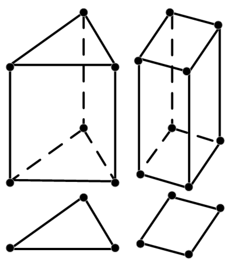
2.2. Discontinuous Galerkin Discretization

The original quadrature-based DG method requires expensive quadrature rules to reduce the aliasing error arising in the nonlinear system that occupies the most computational time of a DG algorithm [37]. Considering that the current second-order accuracy will not cause significant aliasing errors, a quadrature-free approach is adapted to convert the nonlinear fluxes to polynomials or polynomial operations, which can be integrated analytically in the element or element boundaries [38]. To this end, we discretized the above equations based on the quadrature-free nodal discontinuous Galerkin method [33]. A three-dimensional domain Ω 3 d can be projected onto a horizontal domain denoted as Ω 2 d , and then Ω 2 d can be divided into K 2 d horizontal triangular or quadrangular elements that are nonoverlapped. In addition, the number of vertical layers is denoted as N L a y e r , and the K 2 d elements can be extended to K 2 d × N L a y e r triangular or quadrangular prisms. In each prismatic element, a finite dimensional polynomial space, V h , 3 d Ω 3 d , is introduced, and then the linear Lagrange interpolating polynomial, ϕ V h , 3 d , can be defined.
For Equations (1) and (10), we use local numerical solutions, U h , to replace the real solutions, U , and the strong formulations of these equations are written as:
Ω 3 d U h t + E h x + G h y + H h σ ϕ d x = Ω 3 d ϕ n x E h , f E h f , + n y G h , f G h f , + n σ H h , f H h f , d x + Ω 3 d S b , h ϕ d x + D d , h D , K H , K V , f , U h , ϕ .
Here, the left side of the equation contains the time derivative term and the volume integration of the convective term. The first term on the right side is the facial integration of the convective term, where n x E h f , + n y G h f , + n σ H h f , represents the numerical flux at the boundary of each element. The Harten-Lax-van Leer (HLLC) Riemann solver [39] is adopted to calculate the numerical flux at lateral boundaries, while the upwind flux is taken at bottom and top boundaries. Similar to the finite volume method, the use of numerical flux solvers ensures local conservation of the DG scheme. The second term is the volume integration of the bottom topography term. The last term contains the discretization of the vertical diffusion term and the Coriolis term, which are treated implicitly, and the horizontal diffusion term is treated explicitly. Finally, all the terms that are independent of time are moved to the right side of the discrete equation:
d Y d t = L t , Y t ,
where Y t denotes all the discrete degrees of freedom of one step and L represents the semidiscrete system after the discontinuous Galerkin space discretization. More details of the RKDG discretization are available in Ran et al. [40].

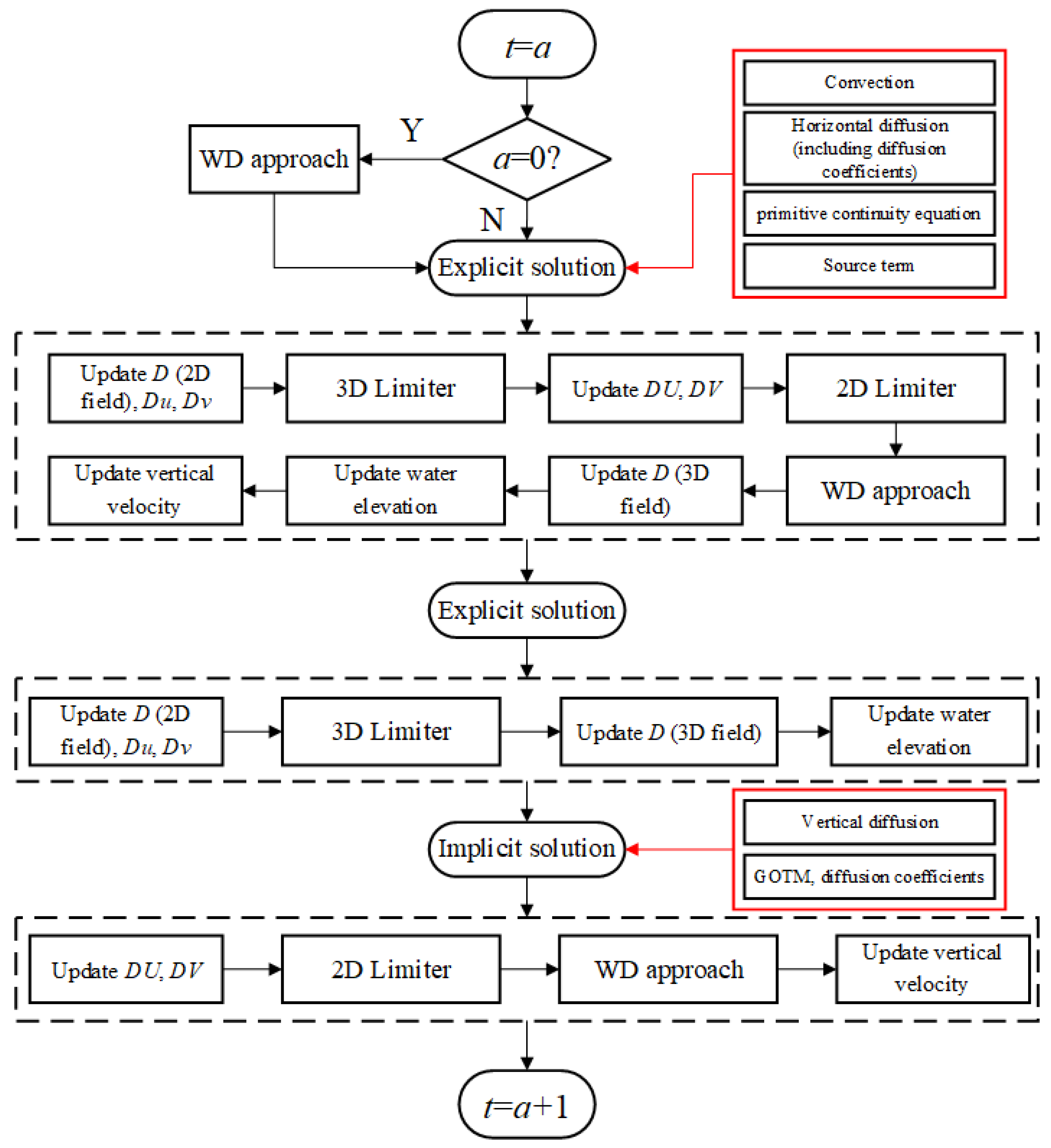
3. Wetting and Drying Treatments

In this section, we provide a complete description of the WD approach, which contains the judgement of the WD nodes and elements, the numerical reconstruction of elements, the calculation of WD elements in the model and the limiter in use to ensure the stability of the model.

3.1. Wet–Dry Nodes and Elements

As mentioned in Section 2, the basic elements used in the model are triangular or quadrangular prisms that are expanded by corresponding horizontal triangles and quadrilaterals, and the interpolating nodes in each element distribute on the vertices of the prisms for the case of a one-order interpolating basis function (Figure 1). For each element, the degree difference of internal angles cannot be too large to keep the stability of the model. The following studies will all take triangles as examples.
Figure 2 shows the judgement process of WD elements. Some processes are inspired from previous 3D circulation models (e.g., POM and FVCOM). We denote D mean as the mean water depth of an element, which is calculated by the interpolating nodes in the element using Gaussian integration, n as the number of wet nodes, and Np as the total number of interpolating nodes in each element. The maximal free surface elevation and the maximal bottom elevation in each element are denoted as η max and z b , max , respectively, where η max = max D + z b . Usually, a positive threshold D crit of a minimum water depth, which is similar to the thickness of the viscous bottom sublayer [13,30], is defined, and then all the nodes can be divided into two categories:
  • wet nodes, for D D crit ;
  • dry nodes, for D < D crit .
Meanwhile, all elements can be first classified into three categories:
  • wet elements, for n = N p ;
  • dry elements, for n = 0 ;
  • semidry elements for 0 < n < N p .
Figure 2. Judgement process of wet and dry elements. Wet elements can be first distinguished by Judge1. Two conditions of elements are defined as dry elements with Judge1 and Judge2. Semidry elements can be divided into flooding elements and dam-breaking elements by Judge3 after reconstructing the water depth and horizontal momentum.
Jmse 12 00147 g002
For semidry elements, when D mean < D crit , these elements are also treated as dry elements. Only if D mean D crit will numerical reconstructions be carried out. Following the method of Xing and Zhang [23], semidry elements are reconstructed with mass conservation. At time level m, the scheme can guarantee the positivity of the water depth and has high-order accuracy, where the formula is:
U j m , x , y = θ U j m x , y U ¯ j m + U ¯ j m
where U ¯ j m = D ¯ j m , D U ¯ j m , D V ¯ j m T , which contains the mean water depth and momentum in an element; U j m and U j m , represent the water depth and momentum at nodes before and after reconstruction; θ 0 , 1 , which is determined by:
θ = min 1 ,   D ¯ j m D ¯ j m D min , j .
Here, D ¯ j m is the mean water depth at node j in an element, which can be ensured to be a positive number under the judgement in Figure 2; D min , j is the minimal water depth of the nodes in an element. It can be shown that once the water depth at any node is nonpositive at a time step, the reconstructed water depth will no longer be negative by using this method. After reconstruction, the semidry elements are further divided into two parts [41,42]: flood elements for η max z b , max and dam-break elements for η max > z b , max . Finally, the elements are classified into four types: wet elements, dry elements, flood elements, and dam-break elements.

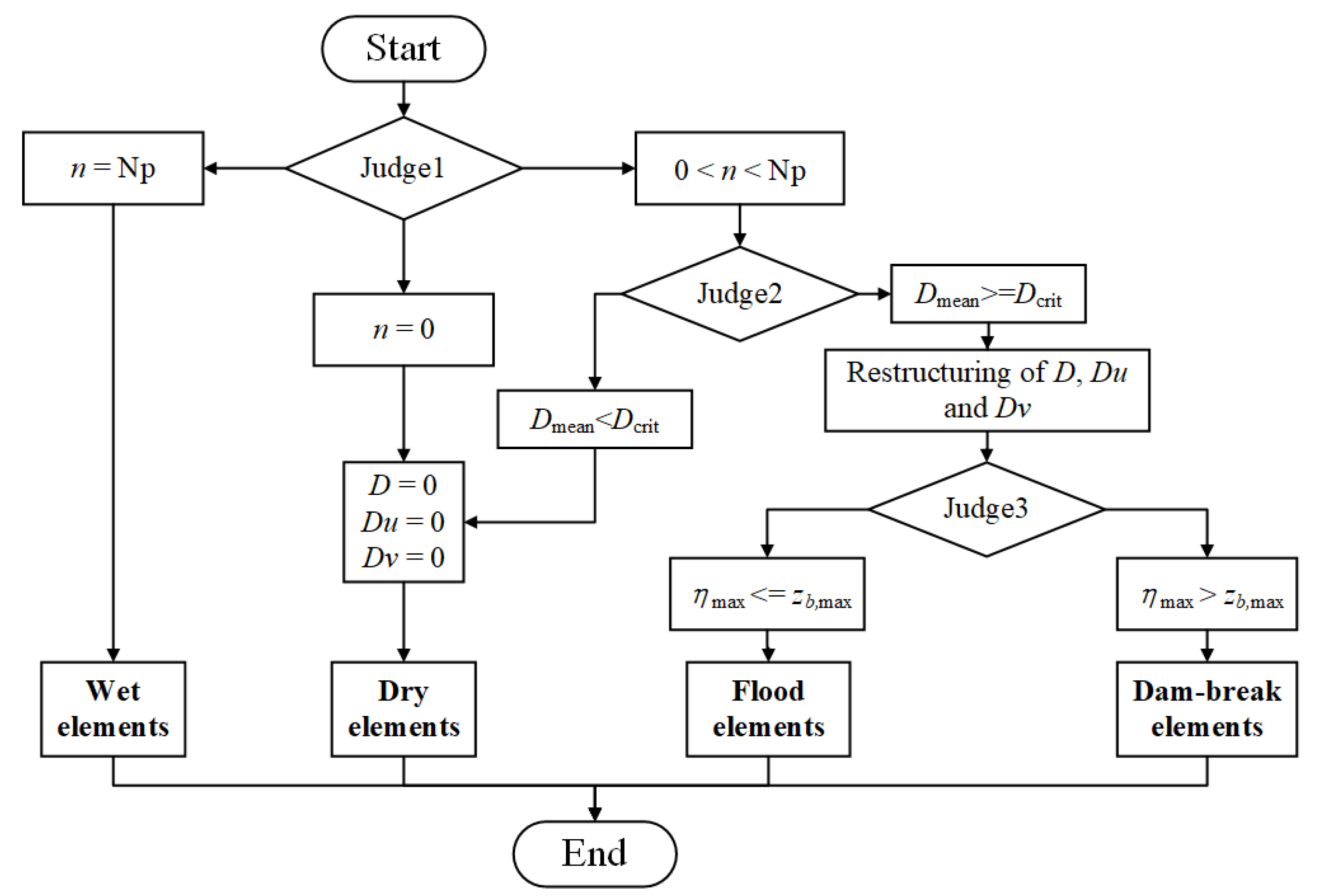
3.2. Calculation of Elements in the Model

In this subsection, we show how the four types of elements work in the model. First, for wet elements, all the processes, including convection, horizontal diffusion, vertical diffusion, the bottom topography term, the Coriolis acceleration term, and the calculation of vertical velocity and surface elevation, need to be run. Second, for dry elements, water movement in the elements is ignored, so there is no need to calculate the volume integration. Nevertheless, the water will flow into the dry elements from wet or semidry elements, where the parts of facial integration, which contain the calculation of numerical flux, need to be run, especially in the convection term. Third, following the method in Lu et al. [43], at the WD interface, the three-dimensional shallow water equations can be treated as two-dimensional shallow water equations, which means that the vertical diffusion and the calculation of vertical velocity do not need to be solved regarding semidry elements. In this model, the horizontal diffusion is not calculated at the WD interface, considering that the effects seem to be minor. For the flood type, gravity g is set to zero to ignore the influence of hydrostatic pressure in the convection term and bottom topography term to guarantee a well-balanced property [42].

3.3. Combined 2D and 3D Limiters

Limiters are decidedly necessary to ensure the stability of the model. Especially at the location of the WD interface, the existence of strong discontinuity can greatly affect the robustness of the model. For a 3D DG model with a mode-splitting scheme, models can simulate WD processes with the help of a 2D limiter at the external mode [28]. In this model, we apply two kinds of limiters. One is a vertex-based 2D limiter to modify the water depth and vertically averaged horizontal momentum, which can be written as:
U k , j m , x = U k , j m x k , j x k + U ¯ k m ,
where k is the element number; x k , j x k expresses the distance between node j and the centroid point in element k; and U k , j m represents the gradients of mean water depth and horizontal momentum following the method of Li and Zhang [27]. The other limiter is a 3D limiter that controls the large gradient of the horizontal momentum, which can be written as:
T k , j = λ T k , j + ( 1 λ ) T ¯ k ,
where T k , j = D u k , j , D v k , j T expresses the original solution at the k triangular prism element, while T ¯ k and T k , j are averaged and limited solutions at the k triangular prism element, respectively; λ is defined by Delandmeter [44].
In the model, a two-order Runge–Kutta time step is adopted, which contains two explicit calculation steps (including the convection term, horizontal diffusion, primitive continuity equation, and source terms) and one implicit calculation step (only for vertical diffusion). In each Runge–Kutta time step, the water depth and the horizontal momentum are updated after the explicit solving process (see Figure 3). The 3D limiter needs to be applied to the whole field immediately or at least before the vertical averaged horizontal momentum ( D U , D V ) is calculated. The 2D limiter can be employed on semidry elements only when D U and D V have been updated, followed by a judgement of the WD statement for elements, which is mentioned in Section 3.1, to finally guarantee that the limited water depth is a nonnegative number.

4. Tests and Analysis of the Wet–Dry Approach

In this section, we first verify the well-balanced property of the model with the WD approach mentioned above and then analyse the performance of WD processing in the long wave runup tests. The in situ tidal flow at Laizhou Bay in the Bohai Sea, China, is also simulated to demonstrate the applicability of the model. The CPU is an Intel (R) Xeon (R) Silver 4110 CPU @ 2.10GHz, using 24 threads for OpenMP parallel computing.

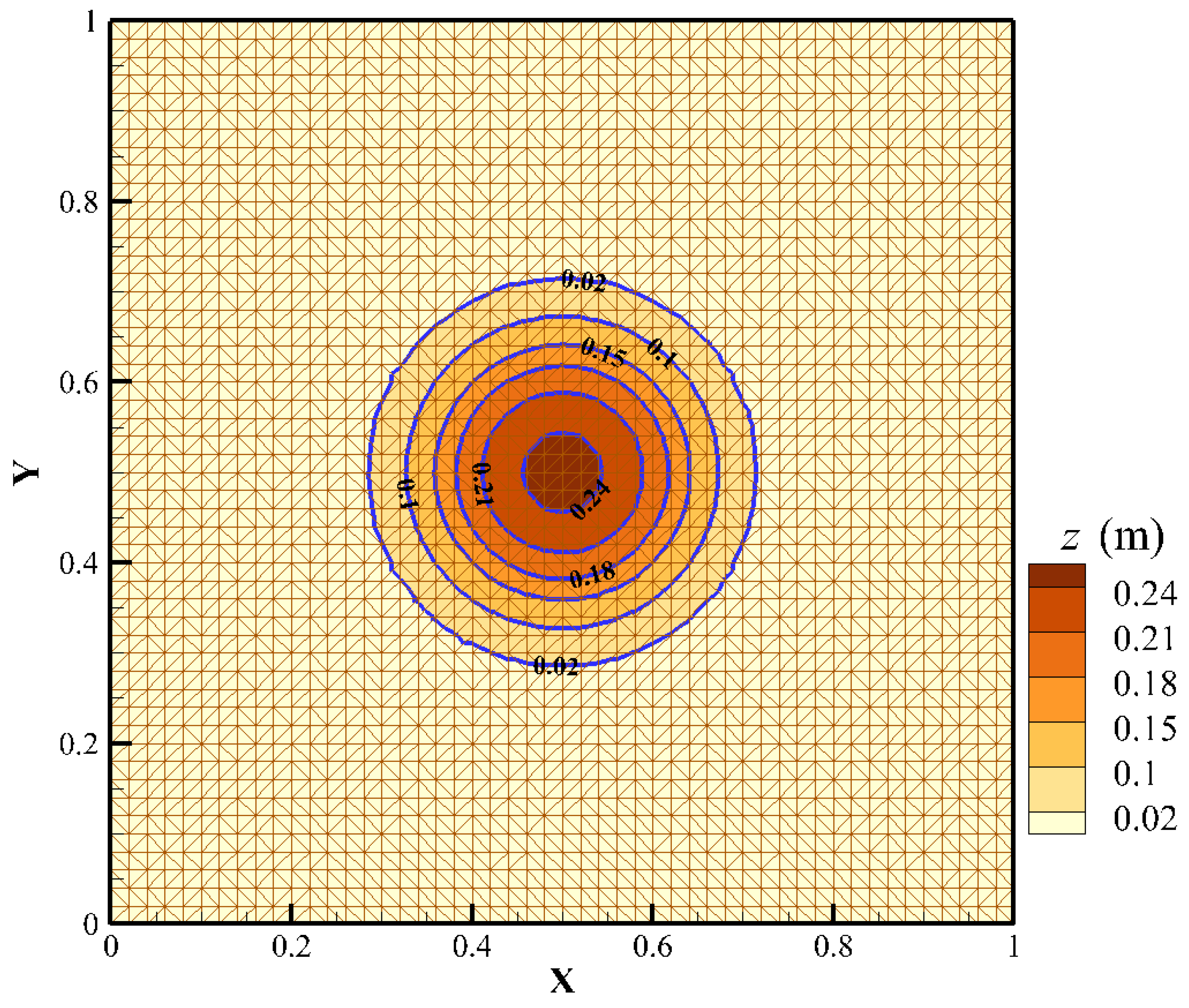
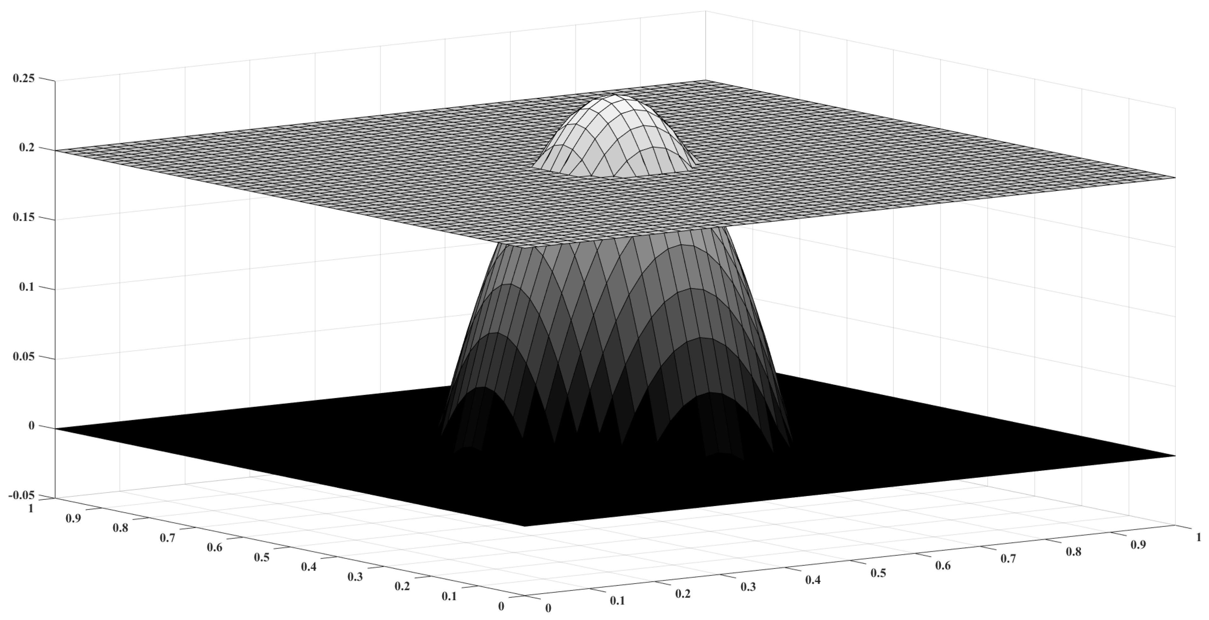
4.1. Well-Balanced Test

The performance of a well-balanced property is essential for a WD treatment, and the purpose of the first test is to show the steady state for the classic problem of “lake at rest”. The case is a steady flow over a bump, obtained from Brufau and García-Navarro [45]. The calculation domain is a square pool from [0, 1] m × [0, 1] m in the x and y directions, where the bottom elevation is defined by:
z b x , y = max 0 , 0.25 5 x 0.5 2 + y 0.5 2 .
Meanwhile, the initial conditions are:
η = max 0.2 , z b ,   D u = 0 ,   D v = 0 .
The boundary sides of the calculation domain are set as nonslip types, and the shape of the horizontal grids is an isosceles right triangle with a scale of 0.02 m (Figure 4). The number of horizontal grids is 5000, while the number of vertical layers is 5. The total simulation time is 30 s, with a constant time step of 0.001 s, and D crit is set to 0.1 mm. The total simulating time is 23.0 min. The water elevation in the domain has nearly no changes, and the results at 30 s are shown in Figure 5. The L1 errors and the L errors of water depth and momentum in the whole domain, which are calculated by the values of all the nodes at 30 s and the initial time, are listed in Table 1, whose orders of magnitude are 10−12 and 10−11, respectively.

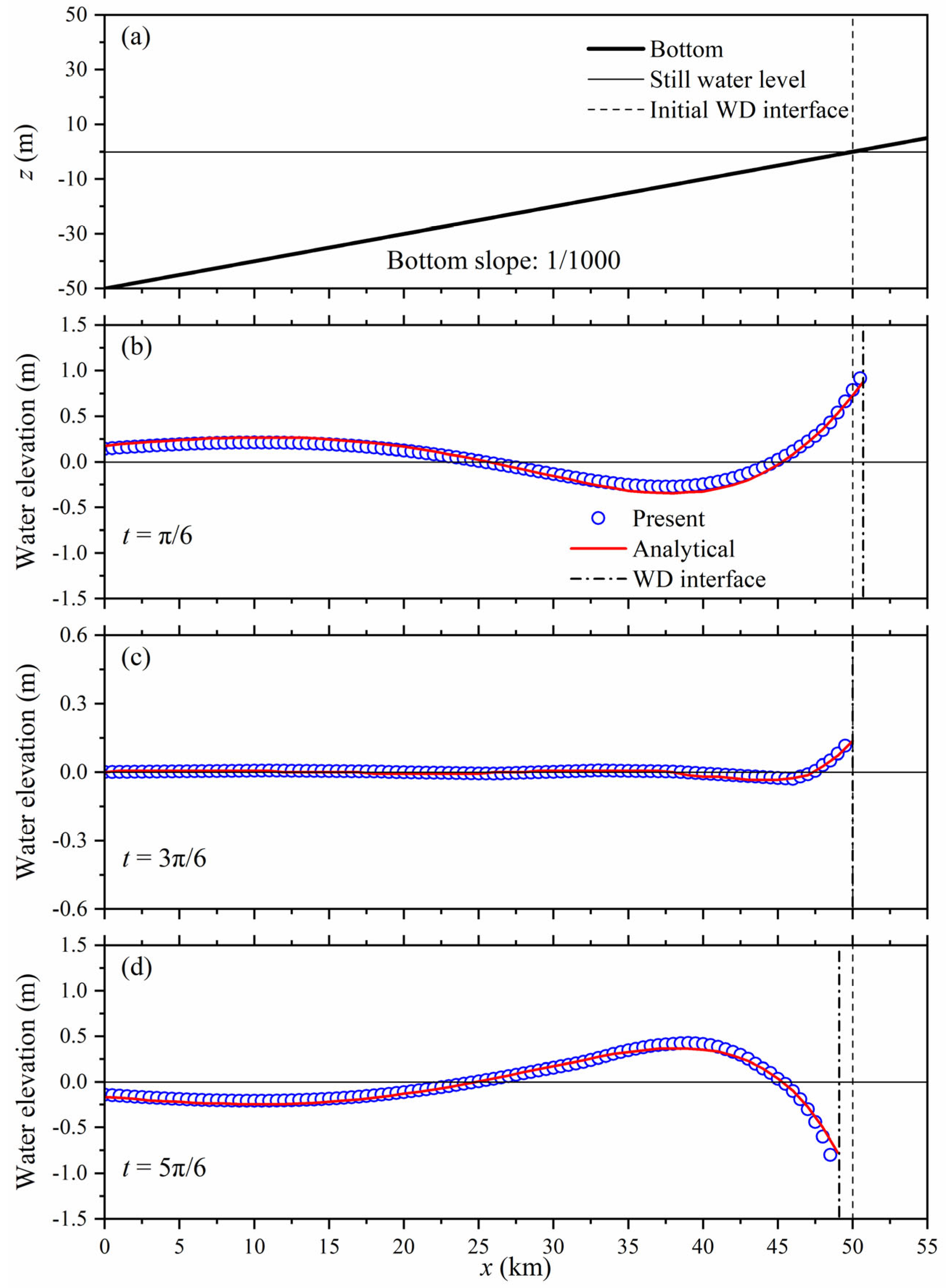
4.2. Long Waves Climbing a Sloping Beach

To verify the performance of WD treatment in the model under dynamic water conditions, we modelled a case where long waves climb a sloping beach, which has analytical solutions derived by Carrier and Greenspan [46]. The calculation domain is set to 55 km in the x direction and 500 m in the y direction. The shape of the horizontal grids is an unstructured isosceles right triangle, but with a scale of 100 m. The bottom slope is 1/1000, and the initial shoreline is at the location x = 50 km. The vertical layers are 5. At x = 0 m, a periodic long wave with a wave height of 0.4 m and a period of 1 h is applied at the open boundary. The total simulation time is 7200 s, with a constant time step of 0.5 s, and D crit is set to 0.01 m. The total simulating time is 40.6 min. Figure 6 shows the simulated water surface elevations and analytical solutions at three timepoints in a wave period, where the simulation results of water elevation are close to the analytical results.

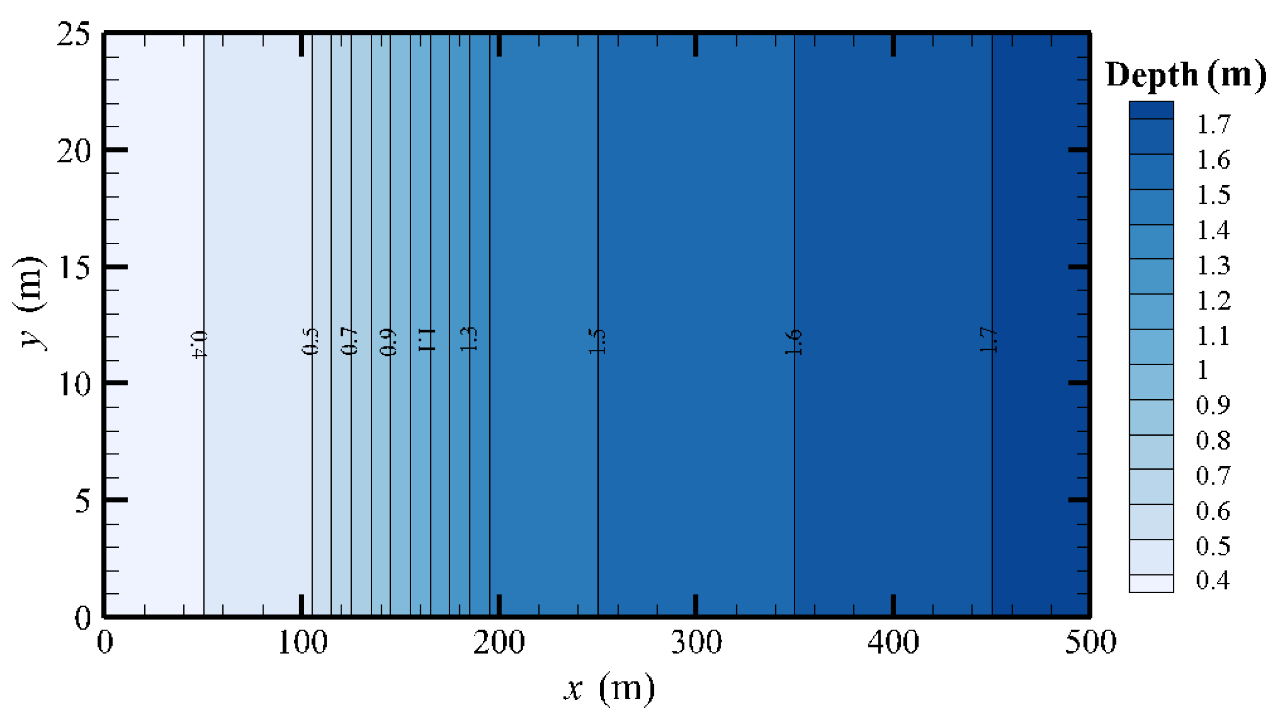
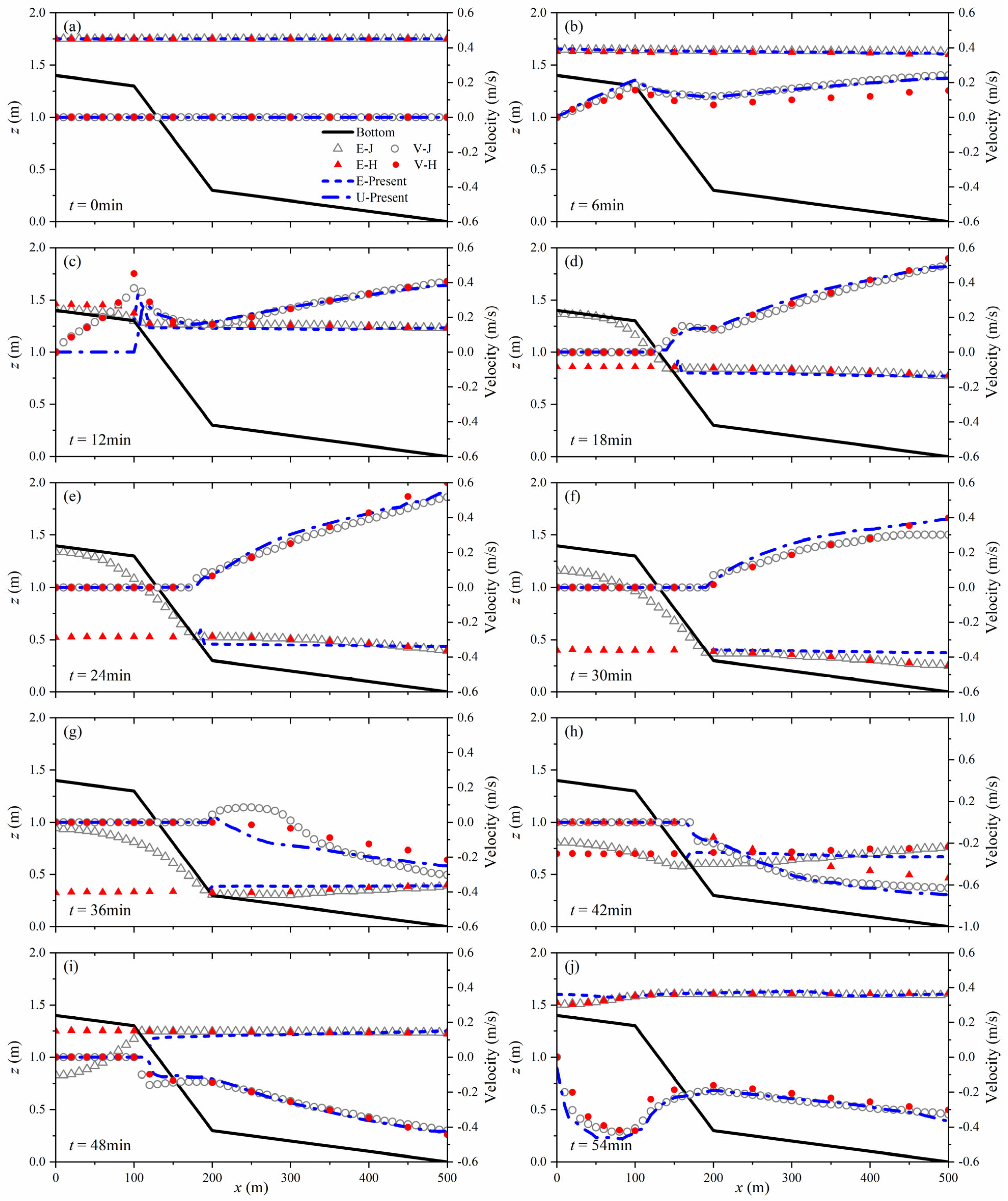
4.3. Basin with Variable Slope under a Tidal Cycle

Next, we compare the modelled results with Jiang and Wai [15] and Heniche et al. [16], using the case of a basin with a variable slope under a tidal cycle presented by Leclerc et al. [47]. The calculation domain is set to 500 m in the x direction and 25 m in the y direction. The bottom slopes from x = 0–100 m and x = 200–500 m are 1/1000 and 1/100 from x = 100–200 m, where the initial water depth in the basin is shown in Figure 7. The scale of the grids is 5 m at x = 0–200 m and 10 m at x = 200–500 m. The total modelled time is 7200 s, with a constant time step of 0.05 s, and D crit is set to 0.05 m. The total simulating time is 52.5 min. The initial water elevation is 1.75 m, and a periodic tide with an amplitude of 0.75 m and a period of 1 h are applied at the open boundary of x = 500 m according to Jiang and Wai [15]:
η = 1.0 + 0.75 cos 2 π t / 3600 .
Parameters that are not mentioned can be found in Jiang and Wai [15]. The simulation results in a tidal cycle of water elevation and mean velocity in the x direction modelled by the above three models, is shown in Figure 8. At t = 0 and t = 6 min, the whole domain is flooded, which does not involve the treatment of the WD approach. The water elevation and velocity modelled by this model are consistent with that of Jiang and Wai [15], while the modelled velocity of Heniche et al. [16] is slightly slower than that of the other two models (Figure 8a,b). At t = 12 min to t = 36 min, with decreasing water level, the area of x < 200 m changes from wet to dry. The results of water elevation by the present model are different from those of the other two models at dry locations because in their models, a negative water depth is allowed, while the water depth in dry regions is set to zero in the present model. At t = 30 min (Figure 8f), the modelled water elevation and velocity of the present model are greater than those of the other two models, but at x = 450–500 m near the open boundary, the results from the present model are similar to those of Heniche et al. [16]. At t = 36 min (Figure 8g), the simulated velocity has gaps among the three models at x = 200–350 m. The decreasing velocities at ebb time modelled by the present model and Heniche et al. [16] seem reasonable. At t = 42 min (Figure 8h), in the range of x = 500 m to 200 m, the simulated water elevation by the present model is maintained at approximately 0.68 m, while it decreases from 0.77 m to 0.60 m by Jiang and Wai [15]. At x = 500 m to 300 m, the velocity modelled by the present model is 0.06 m/s faster than that by Jiang and Wai [15], but the velocity modelled by Heniche et al. [16] is slower than that of the other two models. When the water level increases at t 48 min, the simulated water elevation and velocity of the three models agree with each other again (Figure 8i,j). During the tidal cycle, the difference in results occurs mainly because the treatments at dry regions or WD interfaces further influence the whole region (Jiang and Wai [15] and Heniche et al. [16] use a negative depth algorithm while the present model uses a positivity-preserving and flux correctors method). In general, the present model can reasonably simulate the variation in water elevation and velocity, which is close to the other two models.

4.4. Discussion on the Use of 2D and 3D Limiters

The numerical tests above show the good performance of the WD method in the model, but the roles of the limiters may be confusing, which will be illustrated in this section.
From the literature mentioned in Section 3.3, it is known that 3D limiters in hydrodynamic models work by correcting the maximal and minimal values of horizontal momentum at local elements, while 2D limiters modify water elevation (or water depth) and vertically averaged horizontal momentum. If the model can maintain stability, there is no need to use a limiter to maintain accuracy. Returning to the well-balanced test in Section 4.1, still water does not cause instability problems, so there is no need to use any limiters, and the L1 errors and the L errors of water depth and momentum are fixed (or may be zero), while the employment of 2D and 3D limiters causes variable errors first from the reconstruction of semidry elements and gradually expands to the whole region.
However, when the water moves, not only does the water elevation have a strong discontinuity, but unreasonable extrema at WD interfaces will also occur for horizontal momentum. Taking the long wave climbing test in Section 4.2 as an example, the status of the running model is shown in Table 2. When the model only applies the 3D limiter, the water elevation is likely to be stuck at WD fronts, which finally leads to the breakdown of the model at 3074.0 s. If we use the 2D limiter only, the calculated horizontal momentum errs at 3104.0 s because of unreasonable extreme values when the WD status of elements changes. The model can maintain stability if the 2D and 3D limiters are used together. In short, although the application of limiters may slightly increase the error, it is essential to use both 2D and 3D limiters to prevent oscillation and keep the model more robust.

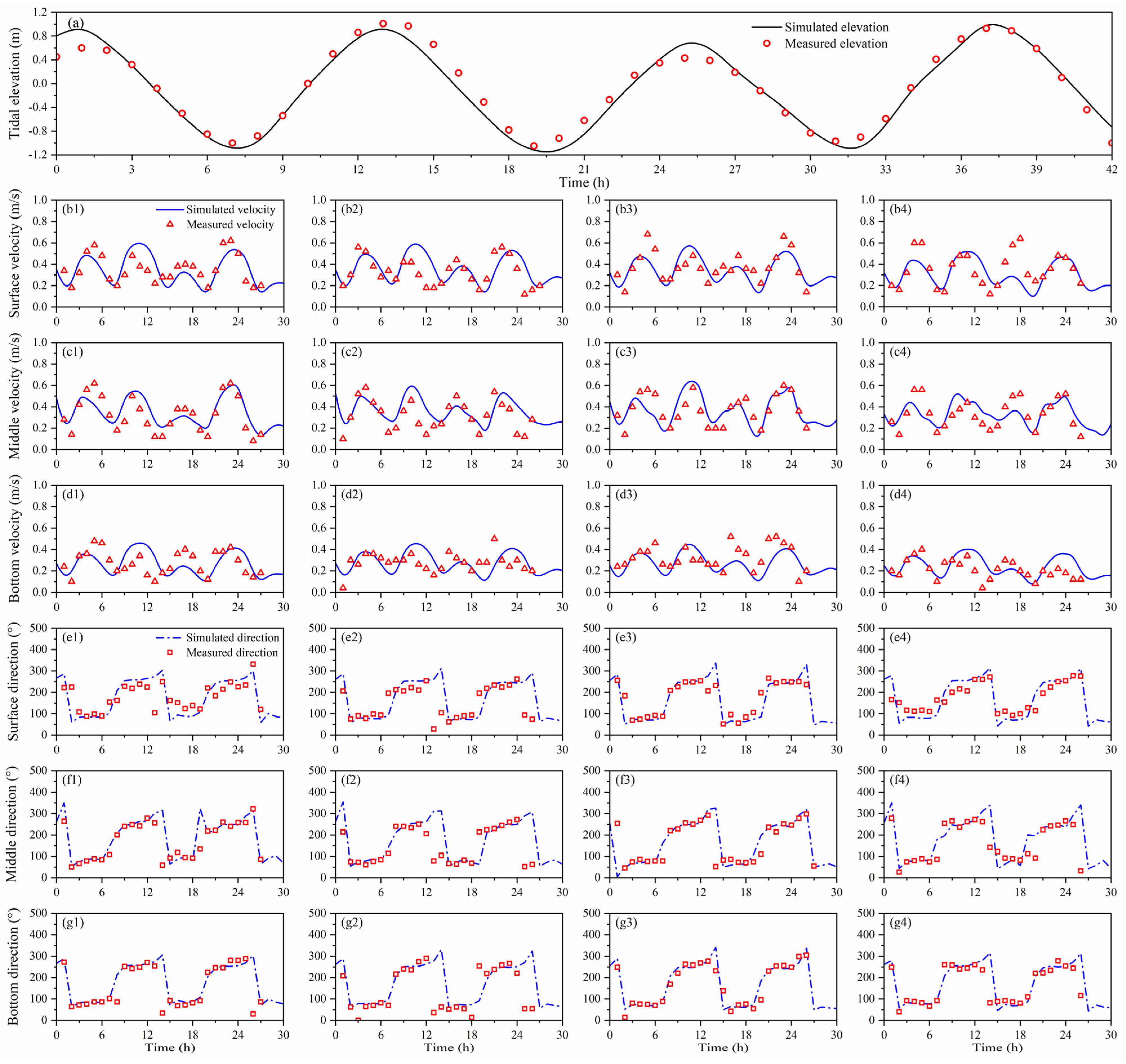
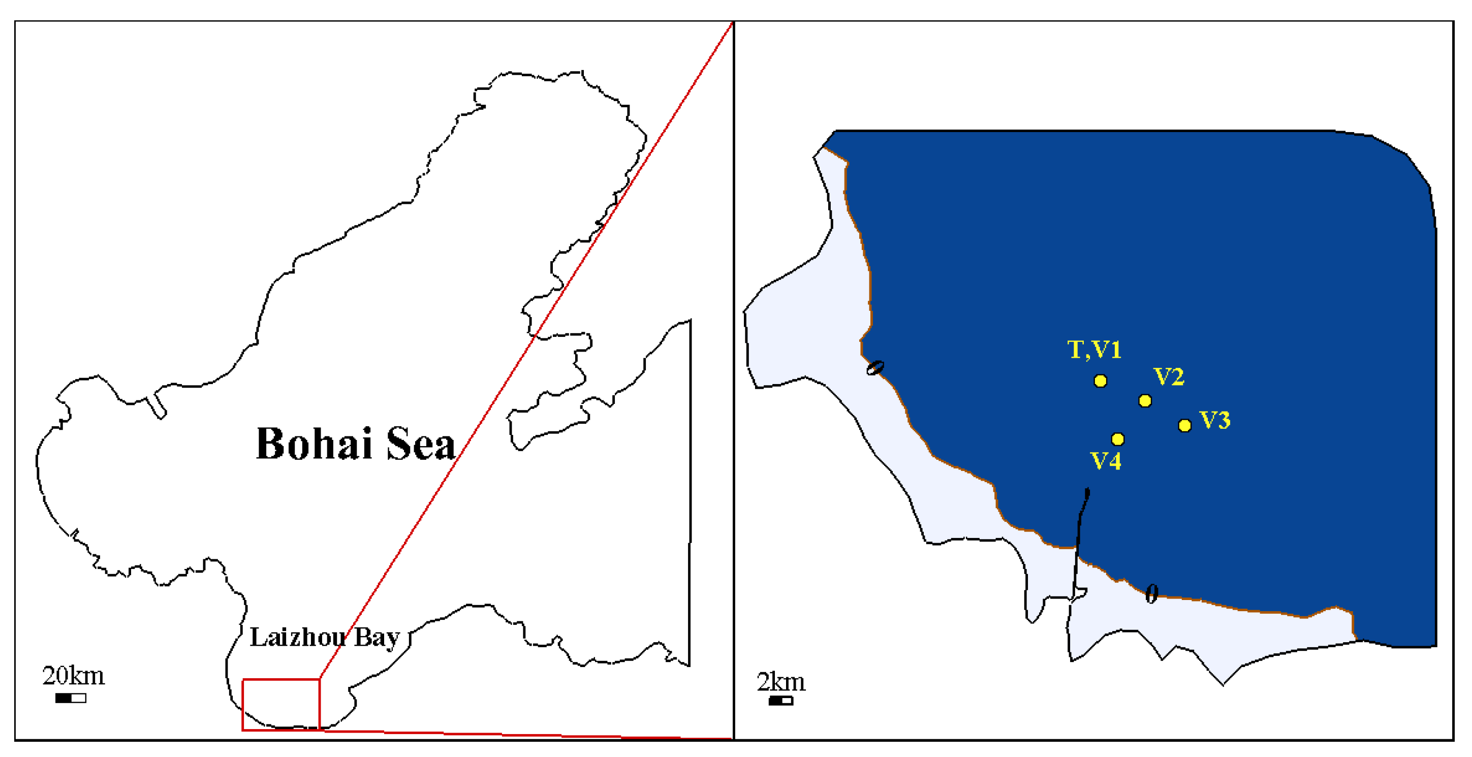
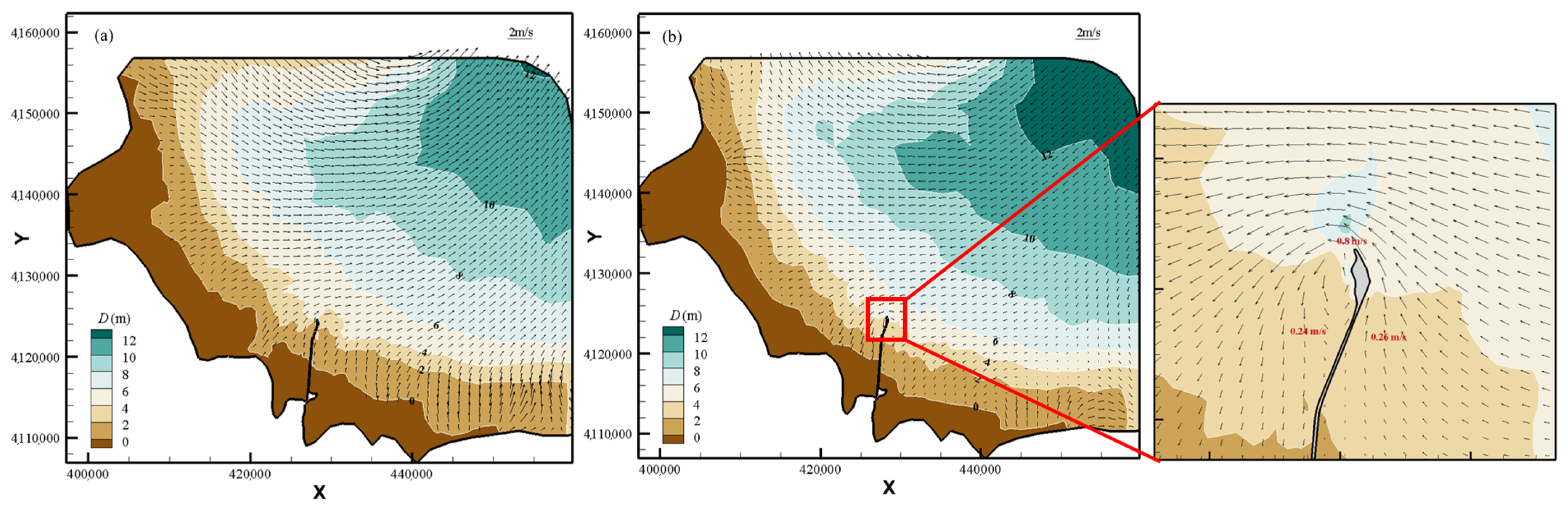
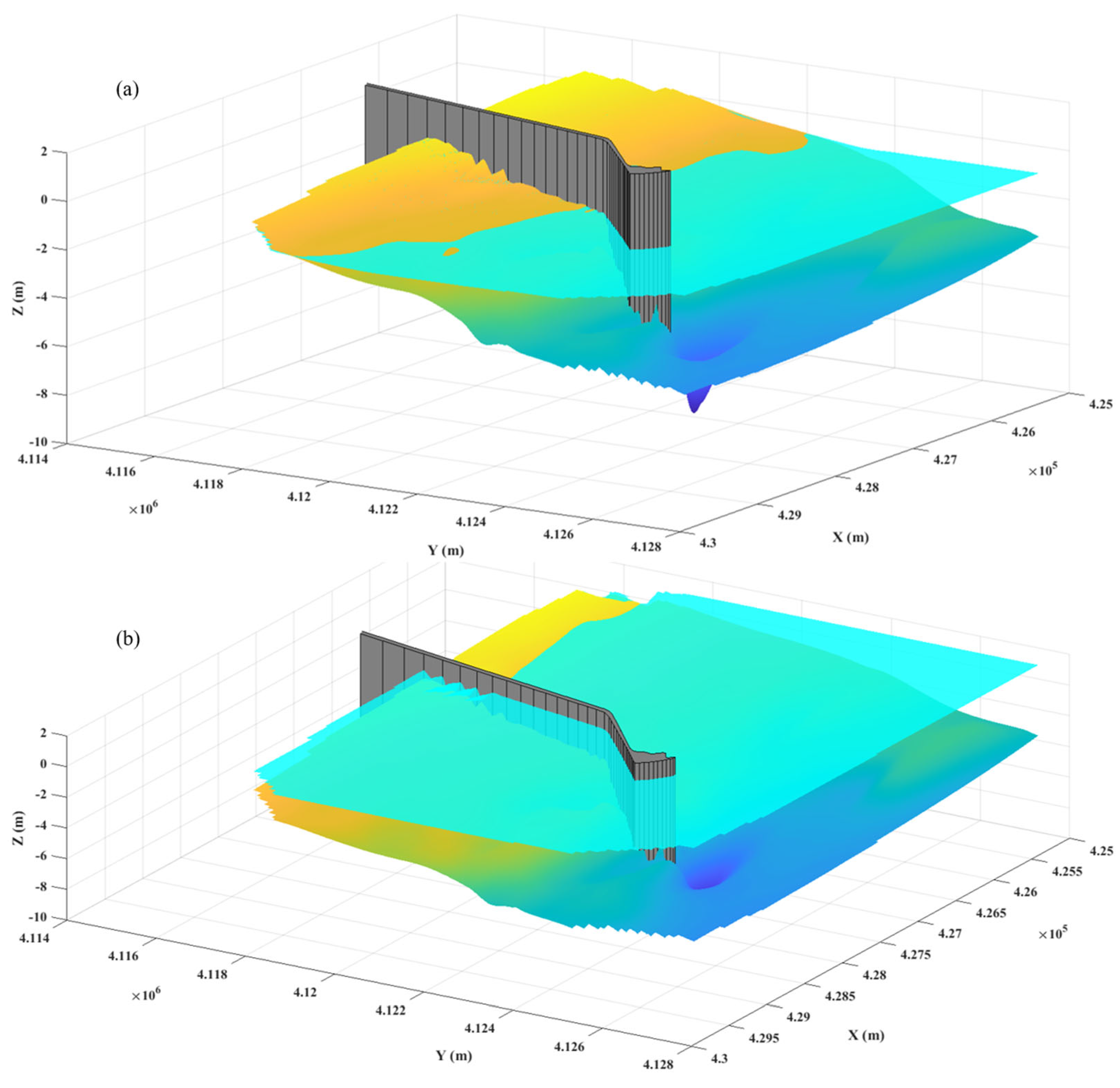
5. Application of the Model for Tidal Flow in Laizhou Bay

In this section, the model is applied to simulate the tidal flow evolution during a spring tidal cycle in the southwest area of Laizhou Bay, Bohai Sea, China, in November 2003. The location of the simulation area is shown in Figure 9. In the right figure, the deepest water depth is approximately 12.7 m, and the initial shoreline (water line) at the mean water surface is also shown. During the flood and ebb processes, the WD fronts will change accordingly. In the computational domain, the maximal grid size is 3500 m, and the minimal is 30 m. The number of horizontal grids is 2328, with 10 layers in the vertical direction. Water elevation data at the open boundaries are obtained from Chinatide [48], which is a tidal forecast system, and the surface wind conditions are primarily from the ERA5 wind-field-reanalysis product. Current data were measured using the SLC9-2 Intelligent Direct Reading Current Meter developed by the Ocean University of China. In the model, simulation results at the top of the second, sixth, and bottom layers correspond to measured data at locations representing the top (0.5 m underwater), middle (0.6 times water depth), and bottom (0.5 m above the seabed) layers, respectively. The time step is 0.25 s, D crit is set to 0.10 m to adapt to the complex topography, the bottom roughness parameter is set to 0.2 mm, which is approximately 2–3 times the median grain size [49], and the Coriolis coefficient is calculated by inputting the latitude of 38° N. The simulation results of water elevation and the current velocity and direction at the top, middle, and bottom layers are all shown in Figure 10. The measured data observed by tidal elevation station T and four current stations V1–V4 are also given to evaluate the performance of the model.
Figure 10a shows that the simulated water elevation generally agrees well with the measured data. At t = 0 ~ 2   h and t = 25 ~ 26   h , the modelled results are slightly higher than the measured data, while at t = 14 ~ 17   h , they are slightly lower. The results of the current direction at the top, middle, and bottom are shown in Figure 10e–g, which are consistent with the measured data overall. For the current velocity, taking the V4 station as an example (Figure 10(b4,c4)), the modelled results seem slower than the measured data at t = 5 ~ 6   h and t = 15 ~ 18   h . In the vertical direction, there is little difference between the surface velocity and the middle velocity, while the bottom velocity is obviously slower than the other two velocities. For the current directions, the differences between the surface, middle, and bottom layers are quite small. The water depth and the flow field over the whole computational region are also shown in Figure 11. It is noted that there is a long jetty connecting a harbor at the head of the jetty with the land in the simulated area. The surface water elevations around the jetty during ebb and flood tides are shown in Figure 12. The flow is blocked by the jetty during flood and ebb processes, which forms a flow field with high velocity of about 0.8 m/s around the jetty head, and the bottom is scoured into a hole of approximately 3.3 m depth. In addition, the surface water elevation at the two sides of the jetty also shows discontinuity, with an approximately 0.4 m height difference at flood tide. The WD status of computing elements in the yellow region changes with time, which ensures that the model correctly distinguishes WD areas and then describes the variable surface water line.
In short, the model could reasonably and accurately reflect the tidal elevation and flow variation during a spring tidal cycle in the southwest area of Laizhou Bay in 2003. By adding the WD treatment method in the 3D DG model, the whole model can satisfactorily simulate the WD front variation in-domain with complex topography.

6. Conclusions

In this work, a wetting and drying treatment for a three-dimensional discontinuous Galerkin hydrodynamic model without using a mode-splitting scheme was developed. In this approach, computing elements were classified into wet elements, dry elements, flooding elements, and dam-breaking elements, which need to be treated differently. In a Runge–Kutta time step, the reconstruction of the semidry elements and the combined utilization of two- and three-dimensional limiters help the model maintain stability. Three numerical tests show that the wetting and drying method can satisfy the well-balanced property and can reasonably describe the variation process of wetting and drying regions. By analyzing the role of the limiters in the model, it was shown that by combining the 2D and 3D limiters in the three-dimensional discontinuous Galerkin hydrodynamic model of the non-split mode can simulate the wetting and drying process effectively, maintaining robustness. The wetting and drying method of the 3D DG model was applied to simulate the tidal flow processes of the spring tidal cycle in the southwest area of Laizhou Bay, Bohai Sea, in November 2003, and the simulation results of the water elevation and vertical layered currents agree well with the measured data, which indicates that the model has good applicability. By adding the WD treatment method, the whole model can satisfactorily simulate the WD front variation in-domain with complex topography.
Future research will focus on the baroclinic model with applications and the balance between calculating accuracy and efficiency.

Author Contributions

Software, Z.C. and G.R.; validation, Z.C. and Y.N.; formal analysis, Z.C.; writing—original draft preparation, Z.C.; writing—review and editing, Z.C. and Q.Z.; supervision, Q.Z.; funding acquisition, Q.Z. All authors have read and agreed to the published version of the manuscript.

Funding

The authors gratefully acknowledge the financial support by National Key Research, Development Project of China (2021YFB2601100) and the Joint Funds of the National Natural Science Foundation of China (Grant No. U1906231), Chongqing Water Conservancy Science and Technology Project (Grant No. CQSLK-2023004) and the research startup funds from Chongqing Jiaotong University (Grant No. F1230085).

Data Availability Statement

No new data were created or analyzed in this study. Data sharing is not applicable to this article.

Conflicts of Interest

The authors declare no conflicts of interest.

References

  1. Marsooli, R.; Orton, P.M.; Georgas, N.; Blumberg, A.F. Three-dimensional hydrodynamic modeling of coastal flood mitigation by wetlands. Coast. Eng. 2016, 111, 83–94. [Google Scholar] [CrossRef]
  2. Safak, I.; List, J.H.; Warner, J.C.; Kumar, N. Observations and 3D hydrodynamics-based modeling of decadal-scale shoreline change along the outer banks, North Carolina. Coast. Eng. 2017, 120, 78–92. [Google Scholar] [CrossRef]
  3. Stansby, P.; Chini, N.; Lloyd, P. Oscillatory flows around a headland by 3D modelling with hydrostatic pressure and implicit bed shear stress comparing with experiment and depth-averaged modelling. Coast. Eng. 2016, 116, 1–14. [Google Scholar] [CrossRef]
  4. Delandmeter, P.; Lambrechts, J.; Legat, V.; Vallaeys, V.; Naithani, J.; Thiery, W.; Remacle, J.-F.; Deleersnijder, E. A fully consistent and conservative vertically adaptive coordinate system for SLIM 3D v0.4 with an application to the thermocline oscillations of Lake Tanganyika. Geosci. Model. Dev. 2018, 11, 1161–1179. [Google Scholar] [CrossRef]
  5. Kärnä, T.; Kramer, S.C.; Mitchell, L.; Ham, D.A.; Piggott, M.D.; Baptista, A.M. Thetis coastal ocean model: Discontinuous Galerkin discretization for the three-dimensional hydrostatic equations. Geosci. Model. Dev. 2018, 11, 4359–4382. [Google Scholar] [CrossRef]
  6. Vallaeys, V.; Lambrechts, J.; Delandmeter, P.; Pätsch, J.; Spitzy, A.; Hanert, E.; Deleersnijder, E. Understanding the circulation in the deep, micro-tidal and strongly stratified Congo River Estuary. Ocean. Model. 2021, 167, 101890. [Google Scholar] [CrossRef]
  7. Le, H.A.; Lambrechts, J.; Ortleb, S.; Gratiot, N.; Deleersnijder, E.; Soares-Frazão, S. An implicit wetting–drying algorithm for the discontinuous Galerkin method: Application to the Tonle Sap, Mekong River Basin. Environ. Fluid. Mech. 2020, 20, 923–951. [Google Scholar] [CrossRef]
  8. Medeiros, S.C.; Hagen, S.C. Review of wetting and drying algorithms for numerical tidal flow models. Int. J. Numer. Meth. Fl. 2013, 71, 473–487. [Google Scholar] [CrossRef]
  9. Ji, Z.G.; Morton, M.R.; Hamrick, J.M. Wetting and drying simulation of estuarine processes. Estuar. Coast. Shelf. Sci. 2001, 53, 683–700. [Google Scholar] [CrossRef]
  10. Martins, R.; Leandro, J.; Djordjević, S. Wetting and drying numerical treatments for the Roe Riemann scheme. J. Hydraul. Res. 2018, 56, 256–267. [Google Scholar] [CrossRef]
  11. Dietrich, J.C.; Kolar, R.L.; Luettich, R.A. Assessment of ADCIRC’s wetting and drying algorithm. Dev. Water. Sci. 2004, 55, 1767–1778. [Google Scholar] [CrossRef]
  12. Oey, L.Y. A wetting and drying scheme for POM. Ocean. Model. 2005, 9, 133–150. [Google Scholar] [CrossRef]
  13. Chen, C.; Qi, J.; Li, C.; Beardsley, R.C.; Lin, H.; Walker, R.; Gates, K. Complexity of the flooding/drying process in an estuarine tidal-creek salt-marsh system: An application of FVCOM. J. Geophys. Res. Oceans 2008, 113, 1–21. [Google Scholar] [CrossRef]
  14. Aureli, F.; Maranzoni, A.; Mignosa, P.; Ziveri, C. A weighted surface-depth gradient method for the numerical integration of the 2D shallow water equations with topography. Adv. Water. Resour. 2008, 31, 962–974. [Google Scholar] [CrossRef]
  15. Jiang, Y.W.; Wai, O.W.H. Drying–wetting approach for 3D finite element sigma coordinate model for estuaries with large tidal flats. Adv. Water Resour. 2005, 28, 779–792. [Google Scholar] [CrossRef]
  16. Heniche, M.; Secretan, Y.; Boudreau, P.; Leclerc, M. A two-dimensional finite element drying-wetting shallow water model for rivers and estuaries. Adv. Water Resour. 1999, 23, 359–372. [Google Scholar] [CrossRef]
  17. Bokhove, O. Flooding and drying in discontinuous Galerkin finite-element discretizations of shallow-water equations. Part 1: One dimension. J. Sci. Comput. 2005, 22–23, 47–82. [Google Scholar] [CrossRef]
  18. Ern, A.; Piperno, S.; Djadel, K. A well-balanced Runge-Kutta discontinuous Galerkin method for the shallow-water equations with flooding and drying. Int. J. Numer. Meth. Fl. 2008, 58, 1–25. [Google Scholar] [CrossRef]
  19. Bunya, S.; Kubatko, E.J.; Westerink, J.J.; Dawson, C. A wetting and drying treatment for the Runge–Kutta discontinuous Galerkin solution to the shallow water equations. Comput. Method. Appl. M. 2009, 198, 1548–1562. [Google Scholar] [CrossRef]
  20. Kesserwani, G.; Liang, Q. Well-balanced RKDG2 solutions to the shallow water equations over irregular domains with wetting and drying. Comput. Fluids. 2010, 39, 2040–2050. [Google Scholar] [CrossRef]
  21. Kärnä, T.; De Brye, B.; Gourgue, O.; Lambrechts, J.; Comblen, R.; Legat, V.; Deleersnijder, E. A fully implicit wetting–drying method for DG–FEM shallow water models, with an application to the Scheldt estuary. Comput. Method. Appl. M. 2011, 200, 509–524. [Google Scholar] [CrossRef]
  22. Meister, A.; Ortleb, S. A positivity preserving and well-balanced DG scheme using finite volume subcells in almost dry regions. Appl. Math. Comput. 2016, 272, 259–273. [Google Scholar] [CrossRef]
  23. Xing, Y.; Zhang, X. Positivity-preserving well-balanced discontinuous Galerkin methods for the shallow water equations on unstructured triangular meshes. J. Sci. Comput. 2013, 57, 19–41. [Google Scholar] [CrossRef]
  24. Xing, Y.; Zhang, X.; Shu, C.-W. Positivity-preserving high order well-balanced discontinuous Galerkin methods for the shallow water equations. Adv. Water Resour. 2010, 33, 1476–1493. [Google Scholar] [CrossRef]
  25. Vater, S.; Beisiegel, N.; Behrens, J. A limiter-based well-balanced discontinuous Galerkin method for shallow-water flows with wetting and drying: One-dimensional case. Adv. Water Resour. 2015, 85, 1–13. [Google Scholar] [CrossRef]
  26. Vater, S.; Beisiegel, N.; Behrens, J. A limiter-based well-balanced discontinuous Galerkin method for shallow-water flows with wetting and drying: Triangular grids. Int. J. Numer. Meth. Fl. 2019, 91, 395–418. [Google Scholar] [CrossRef]
  27. Li, L.X.; Zhang, Q.H. A new vertex-based limiting approach for nodal discontinuous Galerkin methods on arbitrary unstructured meshes. Comput. Fluids. 2017, 159, 316–326. [Google Scholar] [CrossRef]
  28. Vallaeys, V. Discontinuous Galerkin Finite Element Modelling of Estuarine and Plume Dynamics. Ph.D. Thesis, UCL-Université Catholique de Louvain, Ottignies-Louvain-la-Neuve, Belgium, 2018. [Google Scholar]
  29. Kowalik, Z.; Murty, T.S. Numerical Modeling of Ocean Dynamics; World Scientific: Singapore, 1993. [Google Scholar] [CrossRef]
  30. Chen, C.; Qi, J.; Liu, H.; Beardsley, R.C.; Lin, H.; Cowles, G. A wet/dry point treatment method of FVCOM, part I: Stability experiments. J. Mar. Sci. Eng. 2022, 10, 896. [Google Scholar] [CrossRef]
  31. Dawson, C.; Aizinger, V. A discontinuous Galerkin method for three- dimensional shallow water equations. J. Sci. Comput. 2005, 22–23, 245–267. [Google Scholar] [CrossRef]
  32. Conroy, C.J.; Kubatko, E.J. hp discontinuous Galerkin methods for the vertical extent of the water column in coastal settings part I: Barotropic forcing. J. Comput. Phys. 2016, 305, 1147–1171. [Google Scholar] [CrossRef]
  33. Hesthaven, J.S.; Warburton, T. Nodal Discontinuous Galerkin Methods: Algorithms, Analysis, and Applications; Springer Science & Business Media: Berlin, Germany, 2007. [Google Scholar]
  34. Duran, A.; Marche, F. Recent advances on the discontinuous Galerkin method for shallow water equations with topography source terms. Comput. Fluids. 2014, 101, 88–104. [Google Scholar] [CrossRef]
  35. Smagorinsky, J. General circulation experiments with the primitive equations: I. the basic experiment. Mon. Weather Rev. 1963, 91, 99–164. [Google Scholar] [CrossRef]
  36. Burchard, H.; Bolding, K.; Villarreal, M.R. GOTM, a General Ocean Turbulence Model: Theory, Implementation and Test Cases; Technical Report EUR 18745 EN; European Commission: Brussels, Belgium, 1999. [Google Scholar]
  37. Faghih-Naini, S.; Kuckuk, S.; Aizinger, V.; Zint, D.; Grosso, R.; Köstler, H. Quadrature-free discontinuous Galerkin method with code generation features for shallow water equations on automatically generated block-structured meshes. Adv. Water Resour. 2020, 138, 103552. [Google Scholar] [CrossRef]
  38. Li, W. Quadrature-free forms of discontinuous Galerkin methods in solving compressible flows on triangular and tetrahedral grids. Math. Comput. Simulat. 2024, 218, 149–173. [Google Scholar] [CrossRef]
  39. Toro, E.F. Shock-Capturing Methods for Free-Surface Shallow Flows; Wiley-Blackwell: Hoboken, NJ, USA, 2001. [Google Scholar]
  40. Ran, G.Q.; Zhang, Q.H.; Chen, Z.R. Development of a three-dimensional hydrodynamic model based on the discontinuous Galerkin method. Water 2022, 15, 156. [Google Scholar] [CrossRef]
  41. Bates, P.D.; Hervouet, J.M. A new method for moving–boundary hydrodynamic problems in shallow water. Proc. R. Soc. London. Ser. A Math. Phys. Eng. Sci. 1999, 455, 3107–3128. [Google Scholar] [CrossRef]
  42. Li, L.X.; Zhang, Q.H. Development of an efficient wetting and drying treatment for shallow-water modelling using the quadrature-free Runge–Kutta discontinuous Galerkin method. Int. J. Numer. Meth. Fl. 2020, 93, 314–338. [Google Scholar] [CrossRef]
  43. Lu, X.; Mao, B.; Zhang, X.; Ren, S. Well-balanced and shock-capturing solving of 3D shallow-water equations involving rapid wetting and drying with a local 2D transition approach. Comput. Method. Appl. M. 2020, 364, 112897. [Google Scholar] [CrossRef]
  44. Delandmeter, P. Discontinuous Galerkin Finite Element Modelling of Geophysical and Environmental Flows. Ph.D. Thesis, Universite Catholique de Louvain, Ottignies-Louvain-la-Neuve, Belgium, 2017. [Google Scholar]
  45. Brufau, P.; García-Navarro, P. Unsteady free surface flow simulation over complex topography with a multidimensional upwind technique. J. Comput. Phys. 2003, 186, 503–526. [Google Scholar] [CrossRef]
  46. Carrier, G.F.; Greenspan, H.P. Water waves of finite amplitude on a sloping beach. J. Fluid. Mech. 1958, 4, 97–109. [Google Scholar] [CrossRef]
  47. Leclerc, M.; Bellemare, J.F.; Dumas, G.; Dhatt, G. A finite element model of estuarian and river flows with moving boundaries. Adv. Water Resour. 1990, 13, 158–168. [Google Scholar] [CrossRef]
  48. Li, M.; Zheng, J. Introduction to Chinatide software for tide prediction in China seas. J. Waterw. Harb. 2007, 28, 65–68. (In Chinese) [Google Scholar]
  49. Le, H.P.; Cayocca, F.; Waeles, B. Dynamics of sand and mud mixtures: A multiprocess-based modelling strategy. Cont. Shelf. Res. 2011, 31, S135–S149. [Google Scholar] [CrossRef]
Figure 1. Basic elements in the model. Black nodes at the vertices are interpolating nodes for one order interpolating basis functions.
Jmse 12 00147 g001
Figure 3. Calculation process in the model. The explicit solution contains the processes of solving convection, horizontal diffusion, bottom topography terms, and the calculation of surface elevation. The implicit solution contains the processes of solving vertical diffusion with GOTM calculating vertical diffusion coefficients and Coriolis acceleration terms.
Jmse 12 00147 g003
Figure 4. Grids and the bottom topography of the well-balanced test in [45].
Jmse 12 00147 g004
Figure 5. Simulation result of the well-balanced test at 30 s.
Jmse 12 00147 g005
Figure 6. Simulated (blue dots) and analytical (red lines) water surface elevations of a long wave run-up at four different times shown in (ad). Dashed lines are at the locations of the initial wet and dry interface, and dashed-dotted lines are at the locations of the current wet and dry front.
Jmse 12 00147 g006
Figure 7. The initial water depth of the basin in [47].
Jmse 12 00147 g007
Figure 8. Modelled results of water elevation (E) and horizontal velocity (V) in a tidal cycle (from 0 to 54 min in (aj)) by [15] (named E-J and V-J), [16] (named E-H and V-H) and the present model (named E-Present and V-Present).
Jmse 12 00147 g008
Figure 9. Computational domain, WD regions, and locations of the tidal elevation station (T) and four tidal flow velocity stations (V1–V4) in Laizhou Bay.
Jmse 12 00147 g009
Figure 10. The simulated and measured results of (a) the tidal elevation and layered currents. (b1d4) give the layered velocity of the V1–V4 stations, and (e1g4) show the layered direction of the four stations in Laizhou Bay.
Jmse 12 00147 g010
Figure 11. Flow fields and water depth at ebb tide (a) and flood tide (b) in the southwest area of Laizhou Bay in 2003. The local flow field at the jetty head is given. Arrows show the depth-averaged current velocity with directions.
Jmse 12 00147 g011
Figure 12. Variation in surface water elevation at ebb tide (a) and flood tide (b) around a jetty in the southwest area of Laizhou Bay. The cyan surface represents the surface water elevation, and the yellow–blue gradient surface is the bottom terrain. The grey structure is a jetty with a harbor at its head.
Jmse 12 00147 g012
Table 1. Error analysis of the case in [45].
L1 errorL error
DDuDvDDuDv
3.52 × 10−123.77 × 10−133.79 × 10−137.48 × 10−113.76 × 10−113.74 × 10⁻¹¹
Table 2. Running status of the model by using limiters.
Limiters in ModelNo Limiter2D
Limiter
3D
Limiter
Combined 2D and
3D Limiters
StatusBreakdownBreakdownBreakdownNormal
Running time (s)3070.53104.03074.07200.0 (end)
Disclaimer/Publisher’s Note: The statements, opinions and data contained in all publications are solely those of the individual author(s) and contributor(s) and not of MDPI and/or the editor(s). MDPI and/or the editor(s) disclaim responsibility for any injury to people or property resulting from any ideas, methods, instructions or products referred to in the content.

