Identification of Multi-Innovation Stochastic Gradients with Maximum Likelihood Algorithm Based on Ship Maneuverability and Wave Peak Models

Abstract

This paper investigates the problem of real-time parameter identification for ship maneuvering parameters and wave peak frequency in an ocean environment. Based on the idea of Euler discretion, a combined model of ship maneuvering and wave peak frequency (ship–wave) is made a discretion, and a discrete-time auto-regressive moving-average model with exogenous input (ARMAX) is derived for parameter identification. Based on the ideas of stochastic gradient identification and multi-innovation theory, a multi-innovation stochastic gradient (MI-SG) algorithm is derived for parameter identification of the ship–wave discretion model. Maximum likelihood theory is introduced to propose a maximum likelihood-based multi-innovation stochastic gradient (ML-MI-SG) algorithm. Compared to the MI-SG algorithm, the ML-MI-SG algorithm shows improvements in both parameter identification accuracy and identification convergence speed. Simulation results verify the effectiveness of the proposed algorithm.

1. Introduction

As a crucial industry for economic development, the shipping industry is responsible for transporting over 90% of global trade cargo [1,2]. The performance of ship motion control systems directly impacts shipping safety and economic costs. Therefore, an accurate ship maneuvering model is essential to ensure optimal control system performance [3,4]. Given that a ship is a complex system with time-varying nonlinearity, its model parameters change with variations in load, draft, speed, etc. Hence, it is crucial to employ the system identification method to identify unknown model parameters in real-time during ship navigation [5,6]. In addition, a ship is affected differently by wind and waves in different sea conditions [7,8,9]. The peak frequency of waves can be used to judge sea conditions, making the identification of ship maneuvering parameters and peak frequency of waves both important and practically significant.

Ship maneuvering models play a crucial role in the analysis of ship maneuverability, the design of ship maneuvering controllers, and the development of ship maneuvering simulators [10]. Ship maneuvering models provide a high degree of generalization and a theoretical abstraction of the characteristics of the ship motion dynamic system, which can reflect the physical nature of the ship and the quantitative changes in variables during the actual motion process. According to their mathematical forms, ship maneuvering models can be divided into three categories: the Abkowitz holistic mathematical model [11], the MMG separation mathematical model [12], and the response mathematical model [13]. Among them, mathematical models are widely used in the field of control [14,15,16,17,18,19]. They take rudder angle as an input and return bow angle and bow speed as the output. The parameter values of the ship response model are essential for predicting the motion state of the ship [20]. Among them, the K and T indices can be calculated by either the Nomoto standard Z maneuver test method or the regression equation estimation method. In practice, many of the parameters of the ship motion model are calculated or determined by empirical formulas, which are based on ship measurement data [21,22]. System identification based on experimental data is an important method for obtaining the parameters of the motion model [23]. Zhang et al. used the crow search algorithm to address the parameter identification problem of a ship motion model in the autonomous navigation of ships [24]. Allotta et al. proposed a rapid procedure for the fast calibration of the main hydrodynamic parameters of an AUV, and the procedure has been successfully validated using simulation tools and experimental data derived from campaigns at sea [25]. Cardenas et al. proposed an identification method able to estimate a complete set of hydrodynamic coefficients present in the AUV maneuver equations and, using analytical methods, provided an improvement not only to the convergence rate throughout the inclusion of the ASE estimates but also to the estimates’ accuracy [26]. To diminish the parameter drift, reconstruction of the samples and modification of the mathematical model of ship maneuvering motion were carried out in another work. The difference method and the method of additional excitation were proposed to reconstruct the samples in [27]. A new method for hydrodynamic coefficient identification in ship maneuvering mathematical models based on the Bayesian rule was presented, tested, and validated in a nonlinear 4-DOF model with 108 hydrodynamic derivatives [28].

As the ship’s speed, load, and sea state affect the parameters of the ship maneuvering model, it should use recursive estimation algorithms [29,30,31,32,33] to identify the ship maneuvering model through using observation data in real-time [34,35]. Since Kensaku Nomoto’s standard algorithm for obtaining K,T via the Z-test was proposed, ship maneuverability researchers in various countries have been happy to determine K,T using the Z-test for evaluating the ship’s maneuverability performance [36]. It is simple, fast, and accurate to obtain K,T with the system identification method. Currently, commonly used identification algorithms include least squares [37], maximum likelihood estimation [38], Kalman filtering [39], neural networks [40], and support vector machine [41]. Least squares (LS) is a classical identification algorithm that was commonly used before the emergence of intelligent algorithms. However, the algorithm is sensitive to outliers in the training samples, prone to overfitting, and suffers from inconsistent estimation in the identification process [42]. To enhance the applicability and reliability of the least squares algorithm, the stochastic gradient algorithm has been applied to the identification of ship maneuverability models [43,44]. Song et al. proposed a novel nonlinear innovation-based algorithm using the hyperbolic tangent function and a stochastic gradient algorithm [45]. Xie et al. proposed multi-innovation least squares and improved multi-innovation extended Kalman filtering; the recognition accuracy and convergence rate were higher than traditional recognition methods [46]. Zhao et al. proposed a novel identification algorithm for 3-DOF ship maneuvering modeling; the algorithm combined multi-innovation and nonlinear innovation techniques that focus on the innovation’s processing [47].

However, the above methods do not consider the problem that, under wind and wave disturbances, the ship’s heading will sway with the wave disturbances, and the automatic steering gear will strike the rudder when there is a heading deviation [48,49,50]. In order to avoid frequent steering under wind and wave disturbances, wave filters need to be designed [51,52,53]. When using the commonly used filtering methods, the peak frequency acquisition time is long and it is easy to cause excessive phase lag in the control system. In recent years, a number of methods have been developed for identifying the peak frequency of ocean waves. Han et al. proposed a novel algorithm to adaptively search for the optimal cutoff frequency for a low-pass filter with high accuracy. The algorithm is fundamentally based on the fact that the vessel naturally acts as a low-pass filter and the energy from the high-frequency components, e.g., signal noise, is significantly smaller than that from the wave-induced vessel response [54]. For ships with model uncertainty and cross-correlation noise interference, Jiao et al. proposed an improved smooth variable structure filter with cross-correlation noise [55]. Ouyang et al. proposed a robust and easy-to-operate non-parametric modeling method for wave ship maneuvering based on Gaussian process regression (GPR). Difficult-to-measure wave parameters are not required for identifying dynamic models [56]. Zago et al. proposed a new parametric approach for wave estimation based on ship motion, giving a parametric description of the encounter wave spectrum, which allowed the algorithm to perform wave inference in the ship’s frame of ref. [57].

System identification is the theory and method of establishing a mathematical model close to the measured system on the basis of the input and output data of the system [58,59,60,61,62], including the determination of the model structure and the estimation of the model parameters [63,64]. Ding et al. proposed two recursive least squares parameter estimation algorithms by using the data filtering technique, and the auxiliary model identification idea can generate more accurate parameter estimates [65]. To achieve higher accuracy, Guo et al. applied auxiliary model identification ideas and decomposition techniques to derive a two-stage recursive least squares algorithm for estimating the M-OEARMA system [66]. Aiming at the phenomenon of past time-varying parameters in the autoregressive process, with reference to the parameter separation scheme, Xu et al. proposed a recursive identification method based on the decomposition technique of interaction estimation theory for estimating the autoregressive coefficients [67]. To reduce the computational burden, Yang et al. proposed an iterative algorithm for decomposition based on a multi-innovation gradient using the decomposition technique [68,69]. Considering the identification problem of linear continuous time-lag systems, Sun et al. derived a stochastic gradient gradient-based iterative (SG-GI) algorithm capable of estimating unknown parameters and unknown time delays simultaneously by using multi-frequency response and also introduced a forgetting factor to improve the parameter estimation accuracy [70].

The system identification approach enables accurate identification of ship maneuvering parameters and wave frequencies. This is critical for the design of ship maneuvering controllers, observers, and filters. By establishing accurate ship maneuvering models and wave frequency models, the behavior of ships under different maneuvering conditions and wave disturbances can be better understood and predicted. This plays an important role in improving ship maneuvering performance and safety. In this paper, we combine the first-order ship maneuver response model and the first-order wave disturbance model to derive a discrete-time ARMAX ship–wave model for the identification of ship maneuver parameters and wave frequency. In order to achieve this goal, a multi-innovation stochastic gradient (MI-SG) online identification method for ship K-T parameters and wave frequencies is proposed. In comparison to the traditional method, this method can improve the algorithm’s convergence speed and parameter identification accuracy. In addition, in order to further improve the performance of the algorithm, a maximum likelihood multi-innovative stochastic gradient (ML-MI-SG) algorithm based on maximum likelihood theory is proposed. The main contributions of this paper are as follows.

• The ship maneuvering response model and wave disturbance model are converted to an ARMAX model based on the idea of Euler discretization for ship K-T parameters and ocean wave frequency identification.
• Aiming at the ship–wave discrete-time ARMAX model, a ship–wave parameter identification method based on MI-SG algorithms is proposed.
• To improve the identification accuracy by introducing the theory of maximum likelihood, a ML-MI-SG algorithm is proposed to solve the problem.

The paper’s structured as below: Section 2 details the transformation of the ship maneuvering response and wave disturbance model. The MI-SG algorithm, which is based on a ship–wave model, is presented in Section 3. After that, the ML-MI-SG algorithm is presented in Section 4. The calculation method of the ship K-T parameters and wave frequency based on identification parameters is given in Section 5, and the efficiency of the suggested algorithm is validated through simulation in Section 6. Ultimately, in Section 7, we provide concluding remarks.

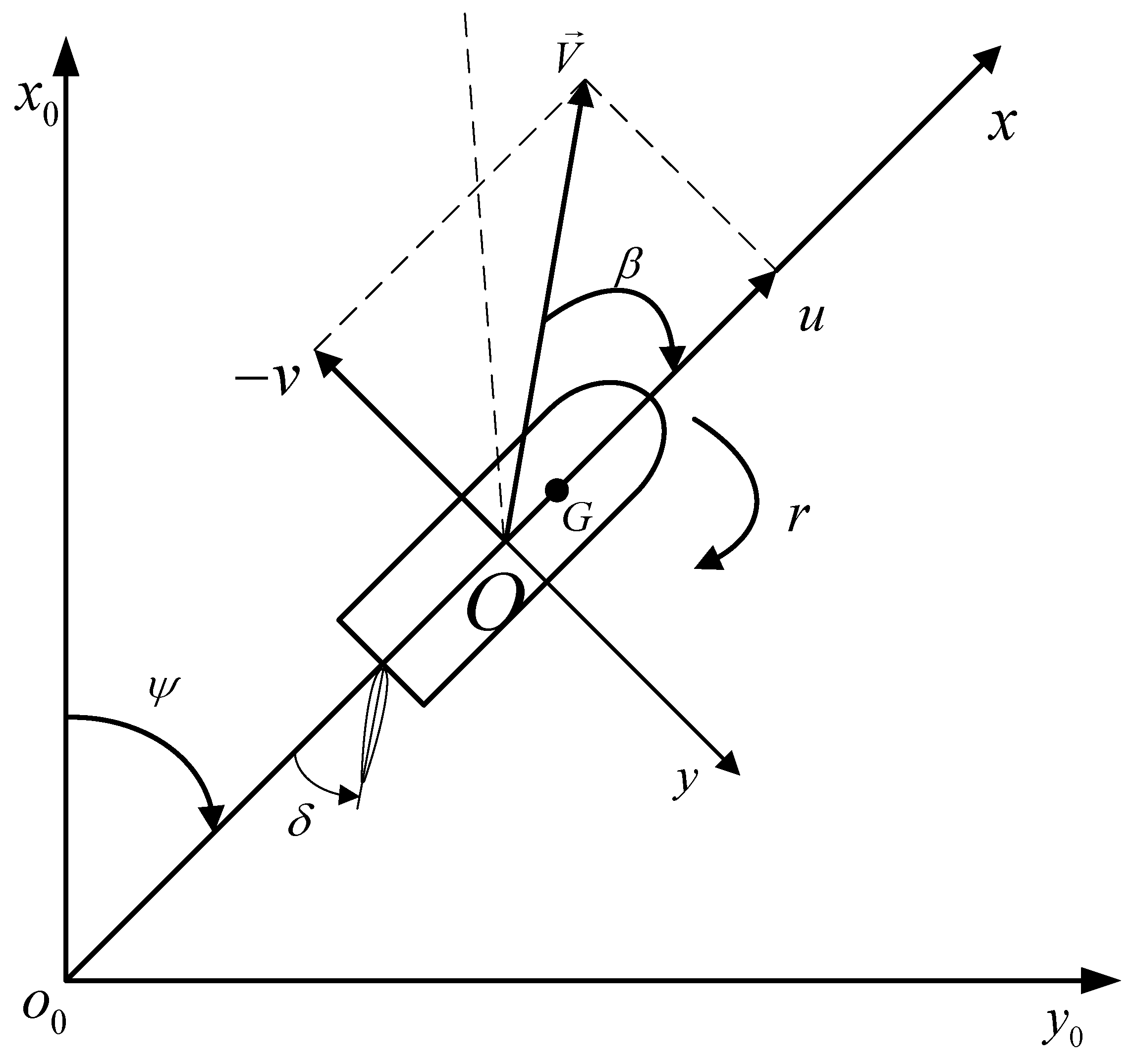
2. Ship–Wave Mathematical Model

The nonlinear ship maneuvering motion and second-order linear wave disturbance models are presented in this section. The motion of the ship’s maneuvering can be described by three degrees of freedom (surge, sway, and yaw), and the hydrodynamic coefficients can be expressed in terms of constants, as illustrated in Figure 1. The equation for ship’s motion in the horizontal plane is given by [71]

$$\begin{array}{cc}\hfill & m\dot{u}-mvr-m{x}_G{r}^2=X,\hfill \\ \hfill & m\dot{v}+mur+m{x}_G\dot{r}=Y,\hfill \\ \hfill & m{x}_G\dot{v}+m{x}_{G}ur+I_{zz}\dot{r}=N,\hfill \end{array}$$

(1)

where the mass and moment of inertia are denoted as m and $I_{zz}$, respectively. The position of the center-of-mass in the x-direction is represented by $x_G$. The hydrodynamic forces and moment are represented by X, Y, and N.

The equation for surge motion can be decoupled from the equations for the motion with three DOFs. By linearizing the sway force and yaw moment, the linear equations [71] are given by

$$\begin{array}{cc}\hfill & \left(m-Y_{\dot{v}}\right)\dot{v}+\left(m{x}_G-Y_{\dot{r}}\right)\dot{r}+mur=Y_{v}v+Y_{r}r+Y_{\delta }\delta ,\hfill \\ \hfill & \left(m{x}_G-N_{\dot{v}}\right)\dot{v}+\left(I_Z-N_{\dot{r}}\right)\dot{r}+m{x}_{G}ur=N_{v}v+N_{r}r+N_{\delta }\delta .\hfill \end{array}$$

(2)

A state-space representation as presented in Fossen [71] gives:

$$\begin{array}{c}\hfill {\mathbf{M}}_R\dot{\mathbf{v}}+{\mathbf{N}}_R\left(\mathbf{v}\right)\mathbf{v}={\mathbf{B}}_R{\delta }_R,\end{array}$$

(3)

where the sway velocity and yaw rate in the body-fixed frame are denoted by $\mathbf{v}={[\mathit{v},r]}^T$, and the rudder deflection is denoted by ${\delta }_R$. The matrices $M_R$, $N_R\left(\mathbf{v}\right)$, and $B_R$ are presented:

$$\begin{array}{cc}\hfill & {\mathbf{M}}_R=\left[\begin{array}{cc}m-Y_{\dot{v}}& m{x}_G-Y_{\dot{r}}\\ m{x}_G-N_{\dot{v}}& I_z-N_{\dot{r}}\end{array}\right],\hfill \\ \hfill & {\mathbf{N}}_R\left(v\right)=\left[\begin{array}{cc}-Y_v& mu-Y_r\\ -N_v& m{x}_{G}u-N_r\end{array}\right],\hfill \\ \hfill & {\mathbf{B}}_R=\left[\begin{array}{c}{Y}_{\delta }\\ N_{\delta }\end{array}\right].\hfill \end{array}$$

(4)

The Abkowitz model [11] comprises nonlinear terms that pose challenges in terms of parameter identification. Thus, a horizontal second-order K-T model is obtained by eliminating the sway velocity $\mathbf{v}$ in Equation (3) without considering the nonlinear terms [36]. The resulting model is given below:

$$\begin{array}{c}\hfill T_1{T}_2\ddot{r}+\left(T_1+T_2\right)\dot{r}+r=K_{\delta }\left({\delta }_R+T_3{\dot{\delta }}_R\right),\end{array}$$

(5)

where $T_1$, $T_2$, $T_3$, and $\mathit{K}$ are the maneuvering indices, which are expressed as:

$$\begin{array}{cc}\hfill & T_1+T_2=\frac{\left(m-Y_{\dot{v}}\right)\left(m{x}_{G}u-N_r\right)-\left(I_Z-N_{\dot{r}}\right)Y_v+\left(m{x}_G-Y_{\dot{r}}\right)N_v+\left(m{x}_G-N_{\dot{v}}\right)\left(mu-Y_r\right)}{-Y_v\left(m{x}_{G}u-N_r\right)+N_v\left(mu-Y_r\right)},\hfill \\ \hfill & T_1{T}_2=\frac{\left(m-Y_{\dot{v}}\right)\left(I_Z-N_{\dot{r}}\right)-\left(m{x}_G-Y_{\dot{r}}\right)\left(m{x}_G-N_{\dot{v}}\right)}{-Y_v\left(m{x}_{G}u-N_r\right)+N_v\left(mu-Y_r\right)},\hfill \\ \hfill & K_{\delta }=\frac{Y_{\delta }{N}_v-N_{\delta }{Y}_v}{-Y_v\left(m{x}_{G}u-N_r\right)+N_v\left(mu-Y_r\right)},\hfill \\ \hfill & T_3=\frac{-Y_{\delta }\left(m{x}_G-N_{\dot{v}}\right)+N_{\delta }\left(m-Y_{\dot{v}}\right)}{Y_{\delta }{N}_v-N_{\delta }{Y}_v}.\hfill \end{array}$$

(6)

This equation is commonly referred to as the second-order Nomoto model [36], and the transfer function is provided as follows:

$$\begin{array}{c}\hfill \frac{r\left(s\right)}{{\delta }_R\left(s\right)}=\frac{-K_{\delta }\left(1+T_{3}s\right)}{\left(1+T_{1}s\right)\left(1+T_{2}s\right)}.\end{array}$$

(7)

In Equation (7), the pole term $(1+T_{2}s)$ and the zero terms $(1+T_{3}s)$ cancel each other out [72]. As $T_2$ and $T_3$ are typically of the same order of magnitude due to their small difference, this is applied to simplify the equation through pole-zero cancellation. The resulting equation is the well-known Nomoto model of the first order.

$$\begin{array}{c}\hfill T\dot{r}+r=K_{\delta }{\delta }_R.\end{array}$$

(8)

We know that in absence of the roll and pitch modes $(\varphi =\theta =0)$, the yawing rate is defined by

$$\begin{array}{c}\hfill \dot{\psi }=r.\end{array}$$

(9)

The following transfer function typically describes the oscillatory motion of the wave.

$$\begin{array}{c}\hfill {\psi }_H\left(s\right)=\frac{K_{w}s}{s^2+2\zeta {\omega }_{n}s+{\omega }_n^2}{w}_H\left(s\right),\end{array}$$

(10)

where $w_H$ is a zero-mean Gaussian white noise and ${\omega }_n$ is the wave peak frequency.

Equation (10) is usually represented by the following state-space representation:

$$\begin{array}{cc}\hfill & {\dot{\psi }}_H=-2\zeta {\omega }_n{\psi }_H-{\omega }_n^2{\xi }_H+K_w{w}_H,\hfill \\ \hfill & {\dot{\xi }}_H={\psi }_H.\hfill \end{array}$$

(11)

Therefore, considering the ship motion and second-order wave disturbances models:

$$\begin{array}{cc}\hfill & {\dot{r}}_L\left(k\right)=\frac{-r_L\left(k\right)+K_{\delta }{\delta }_R\left(k\right)}{T},\hfill \\ \hfill & {\dot{\psi }}_L\left(k\right)=r_L\left(k\right),\hfill \\ \hfill & {\dot{\psi }}_H\left(k\right)=-2\zeta {\omega }_n{\psi }_H\left(k\right)-{\omega }_n^2{\xi }_H\left(k\right)+K_{w}w\left(k\right),\hfill \\ \hfill & {\dot{\xi }}_H\left(k\right)={\psi }_H\left(k\right).\hfill \end{array}$$

(12)

Generally, the total ship yaw angle consists of a low-frequency ship yaw angle and a high-frequency wave disturbance yaw angle. The total yaw angle of the ship can therefore be written as

$$\begin{array}{c}\hfill \psi \left(s\right)={\psi }_L\left(s\right)+{\psi }_H\left(s\right).\end{array}$$

(13)

This system can be written in state-space form

$$\begin{array}{cc}\hfill & \dot{x}\left(k\right)=Ax\left(k\right)+B\delta \left(k\right)+Ew\left(k\right),\hfill \\ \hfill & y\left(k\right)=Cx\left(k\right),\hfill \end{array}$$

(14)

where $x\left(k\right)={[r_L\left(k\right),{\psi }_L\left(k\right),{\psi }_H\left(k\right),{\xi }_H\left(k\right)]}^T$, $\delta \left(k\right)$ is the rudder angle, $w\left(k\right)$ is a zero-mean Gaussian white noise sequence, $y\left(k\right)=\psi \left(k\right)={\psi }_L\left(k\right)+{\psi }_H\left(k\right)$, and

$$\begin{array}{c}\hfill A=\left[\begin{array}{cccc}-1/T& 0& 0& 0\\ 1& 0& 0& 0\\ 0& 0& -2\zeta {\omega }_n& -{\omega }_n^2\\ 0& 0& 1& 0\end{array}\right],B=\left[\begin{array}{c}K/T\\ 0\\ 0\\ 0\end{array}\right],E=\left[\begin{array}{c}0\\ 0\\ K_w\\ 0\end{array}\right],C=\left[\begin{array}{c}0\\ 1\\ 1\\ 0\end{array}\right].\end{array}$$

(15)

Next, we can transform this model representation to a discrete-time ARMAX model:

$$\begin{array}{c}\hfill A_{\alpha }\left(z^{-1}\right)y\left(k\right)=B_{\alpha }\left(z^{-1}\right)u\left(k\right)+C_{\alpha }\left(z^{-1}\right)e\left(k\right).\end{array}$$

(16)

The polynomials $A_{\alpha }\left(z^{-1}\right)$, $B_{\alpha }\left(z^{-1}\right)$, and $C_{\alpha }\left(z^{-1}\right)$ will depend on the discretization method used. In this paper, we discretize Equation (14) using the Euler discretization method [71]. The Euler discretization formula is

$$\begin{array}{cc}\hfill & x\left(k+1\right)=\Phi x\left(k\right)+\Delta u\left(k\right)+\Gamma e\left(k\right),\hfill \\ \hfill & y\left(k\right)=Cx\left(k\right),\hfill \end{array}$$

(17)

where $\Phi =exp\left(Ah\right),\Delta =A^{-1}\left(\Phi -I\right)B,\Gamma =A^{-1}\left(\Phi -I\right)E.$ Hence,

$$\begin{array}{c}\hfill y\left(k\right)=C{\left(zI-\Phi \right)}^{-1}\Delta u\left(k\right)+C{\left(zI-\Phi \right)}^{-1}\Gamma e\left(k\right).\end{array}$$

(18)

Using the fact that:

$$\begin{array}{c}\hfill {\left(zI-\Phi \right)}^{-1}=\frac{adj\left(zI-\Phi \right)}{det\left(zI-\Phi \right)}.\end{array}$$

(19)

From Equations (18) and (19) we have

$$\begin{array}{c}\hfill det\left(zI-\Phi \right)y\left(k\right)=Cadj\left(zI-\Phi \right)\Delta u\left(k\right)+Cadj\left(zI-\Phi \right)\Gamma e\left(k\right),\end{array}$$

(20)

where $A_{\alpha }\left(z^{-1}\right)=det\left(zI-\Phi \right),B_{\alpha }\left(z^{-1}\right)=Cadj\left(zI-\Phi \right)\Delta ,C_{\alpha }\left(z^{-1}\right)=Cadj\left(zI-\Phi \right)\Gamma$.

In order to establish the identification model, the ship–wave model can be expressed as an ARMAX model according to Equation (16), where

$$\begin{array}{cc}\hfill & A_{\alpha }\left(z^{-1}\right):=1+a_1{z}^{-1}+a_2{z}^{-2}+a_3{z}^{-3}+a_4{z}^{-4},\hfill \\ \hfill & B_{\alpha }\left(z^{-1}\right):=b_1{z}^{-2}+b_2{z}^{-3}+b_3{z}^{-4},\hfill \\ \hfill & C_{\alpha }\left(z^{-1}\right):=c_1{z}^{-1}+c_2{z}^{-2}+c_3{z}^{-3}+c_4{z}^{-4}.\hfill \end{array}$$

According to the above formula, we can obtain the following relationship:

$$\begin{array}{cc}\hfill y\left(k\right)& =a_{1}y\left(k-1\right)+a_{2}y\left(k-2\right)+a_{3}y\left(k-3\right)+a_{4}y\left(k-4\right)\hfill \\ \hfill & +b_{1}u\left(k-2\right)+b_{2}u\left(k-3\right)+b_{3}u\left(k-4\right)\hfill \\ \hfill & +c_{1}e\left(k-1\right)+c_{2}e\left(k-2\right)+c_{3}e\left(k-3\right)+c_{4}e\left(k-4\right),\hfill \end{array}$$

(21)

where

$$\begin{array}{cc}\hfill & a_1=\frac{4T-h-2\zeta {\omega }_{n}hT}{T},\hfill \\ \hfill & a_2=\frac{2h-6T+6\zeta {\omega }_{n}hT-2\zeta {\omega }_n{h}^2-{\omega }_n^2{h}^{2}T}{T},\hfill \\ \hfill & a_3=\frac{4T-3h-6\zeta {\omega }_{n}hT+4\zeta {\omega }_n{h}^2-2{\omega }_n^2{h}^{2}T-{\omega }_n^2{h}^3}{T},\hfill \\ \hfill & a_4=\frac{h-T+2\zeta {\omega }_{n}hT-2\zeta {\omega }_n{h}^2-{\omega }_n^2{h}^{2}T-{\omega }_n^2{h}^3}{T},\hfill \\ \hfill & b_1=\frac{k{h}^2}{T},\hfill \\ \hfill & b_2=\frac{2k{h}^2(\zeta {\omega }_{n}h-1)}{T},\hfill \\ \hfill & b_3=\frac{k{h}^2({\omega }_n^2{h}^2-2\zeta {\omega }_{n}h+1)}{T},\hfill \\ \hfill & c_1=1,\hfill \\ \hfill & c_2=\frac{h-3T}{T},\hfill \\ \hfill & c_3=\frac{3T-2h}{T},\hfill \\ \hfill & c_4=\frac{h-T}{T}.\hfill \end{array}$$

Equation (21) can be rewritten as

$$\begin{array}{cc}\hfill y\left(k\right)& ={\gamma }_s^T\left(k\right){\tau }_s+{\gamma }_n^T\left(k\right){\tau }_n+v\left(k\right)\hfill \\ \hfill & ={\gamma }^T\left(k\right)\tau +v\left(k\right),\hfill \end{array}$$

(22)

where

$$\begin{array}{cc}\hfill & {\tau }_s:={\left[a_1,a_2,a_3,a_4,b_1,b_2,b_3\right]}^{\mathrm{T}}\in R^{n_1},\hfill \\ \hfill & {\tau }_n:={\left[c_1,c_2,c_3,c_4\right]}^{\mathrm{T}}\in R^{n_2},\hfill \\ \hfill & \tau :={\left[{\tau }_s^{\mathrm{T}},{\tau }_n^{\mathrm{T}}\right]}^{\mathrm{T}}\in R^{n_0},\hfill \\ \hfill & {\gamma }_s^{\mathrm{T}}\left(k\right):=\left[y\left(k-1\right),y\left(k-2\right),y\left(k-3\right),y\left(k-4\right),u\left(k-2\right),u\left(k-3\right),u\left(k-4\right)\right]\in R^{n_1},\hfill \\ \hfill & {\gamma }_n^{\mathrm{T}}\left(k\right):=\left[e\left(k-1\right),e\left(k-2\right),e\left(k-3\right),e\left(k-4\right)\right]\in R^{n_2},\hfill \\ \hfill & {\gamma }^{\mathrm{T}}\left(k\right):=\left[{\gamma }_s^{\mathrm{T}}\left(k\right),{\gamma }_n^{\mathrm{T}}\left(k\right)\right]\in R^{n_0},\hfill \end{array}$$

where ${\tau }_s,{\tau }_n$, and $\tau$ are the parameter vectors requiring identification, and ${\gamma }_s\left(k\right),{\gamma }_n\left(k\right)$, and $\gamma \left(k\right)$ are the information vectors.

In practice, there are other affecting uncertainties. Equation (21) can be expressed as an ARMAX model

$$\begin{array}{c}\hfill A_{\alpha }\left(z^{-1}\right)y\left(k\right)=B_{\alpha }\left(z^{-1}\right)u\left(k\right)+w\left(k\right).\end{array}$$

(23)

The proposed parameter estimation algorithms in this paper are based on the parameter identification model in (22). Many identification methods are derived based on the identification models of systems [73,74,75,76,77] and can be used to estimate the parameters of other linear systems and nonlinear systems [78,79,80,81,82] and can be applied to other fields [83,84,85,86,87] such as information processing and process control systems. The objective is to develop innovative identification algorithms that can objectively evaluate parameters of ship’s motion and the frequency of the wave’s peak.

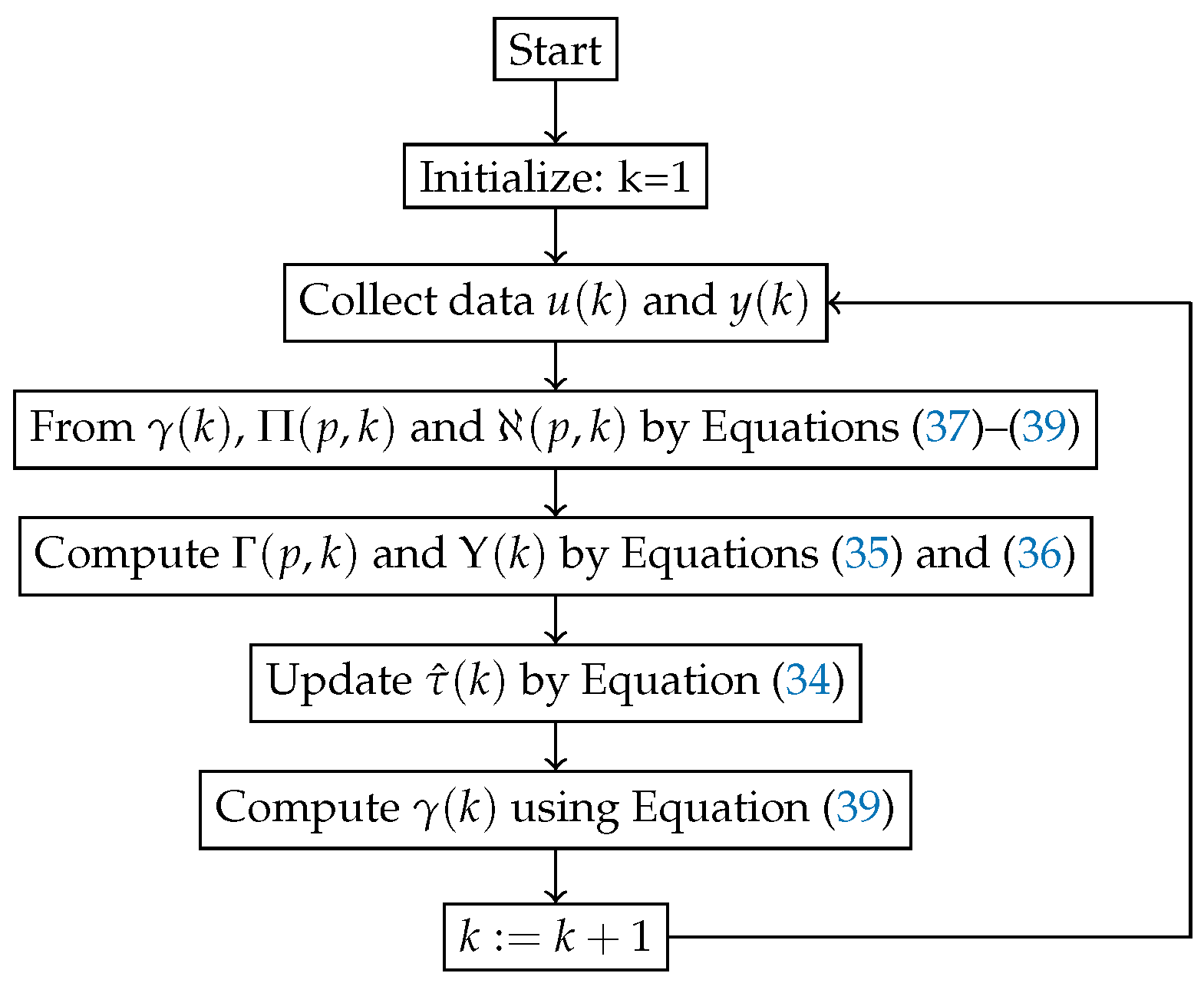
3. The Multi-Innovation Stochastic Gradient Algorithm

In this section, an MI-SG algorithm based on the input–output representation of the ship–wave model is proposed by combining the multi-innovation theory with the stochastic gradient algorithm. The stochastic gradient (SG) algorithm [88,89] can ascertain the parameter matrix $\tau$ in Equation (22):

$$\begin{array}{cc}\hfill \widehat{\tau }\left(k\right)& =\widehat{\tau }(k-1)+\frac{\gamma \left(k\right)}{{\rm Y}\left(k\right)}ϵ\left(k\right),\hfill \end{array}$$

(24)

$$\begin{array}{cc}\hfill ϵ\left(k\right)& =y^T-{\gamma }^T\left(k\right)\widehat{\tau }(k-1),\hfill \end{array}$$

(25)

$$\begin{array}{cc}\hfill {\rm Y}\left(k\right)& ={\rm Y}(k-1)+{\parallel \gamma \left(k\right)\parallel }^2,{\rm Y}\left(0\right)=1.\hfill \end{array}$$

(26)

Here, $ϵ\left(k\right)\in R^{1\times m}$ is a row vector that shows an innovation and element of $ϵ\left(k\right)$ is an individual innovation at present moment.

To enhance the convergence rate of the SG algorithm, a MI-SG algorithm is presented. Refer to [90,91,92,93,94,95,96] and update the SG algorithm by expanding the scalar innovation $ϵ\left(k\right)$ to a multi-innovation vector:

$$\begin{array}{c}\hfill \Gamma (p,k)=\left[\begin{array}{c}ϵ\left(k\right)\\ ϵ(k-1)\\ ⋮\\ ϵ(k-p+1)\end{array}\right]\in R^{1\times p},\end{array}$$

(27)

where p refers to the length of innovation, and

$$\begin{array}{c}\hfill ϵ(k-i)=y(k-i)-{\gamma }^T(k-i)\widehat{\tau }(k-i-1)\in R^{1\times p}.\end{array}$$

(28)

Normally, the estimation of $\widehat{\tau }(k-1)$ is closer than $\widehat{\tau }(k-i)$ at $k-i(i=2,3,4,\dots ,p-1)$. Therefore, it is more sensible to take the innovation vector.

$$\begin{array}{c}\hfill \Gamma (p,k)=\left[\begin{array}{c}y\left(k\right)-{\gamma }^T\left(k\right)\widehat{\tau }(k-1)\\ y(k-1)-{\gamma }^T(k-1)\widehat{\tau }(k-1)\\ ⋮\\ y(k-p+1)-{\gamma }^T(k-p+1)\widehat{\tau }(k-1)\end{array}\right]\in R^{1\times p}.\end{array}$$

(29)

The stacked information matrix $\Pi (p,k)$ and stacked output vector $\aleph (p,k)$ are defined as

$$\begin{array}{cc}\hfill \Pi (p,k)& =[\gamma \left(k\right),\gamma (k-1),\dots ,\gamma (k-p+1)]\in R^{n_0\times p},\hfill \end{array}$$

(30)

$$\begin{array}{cc}\hfill \aleph (p,k)& ={[y\left(k\right),y(k-1),\dots ,y(k-p+1)]}^T\in R^p,\hfill \end{array}$$

(31)

$\Gamma (p,k)$ as the innovation vector is an expression of an equivalent form

$$\begin{array}{c}\hfill \Gamma (p,k)=\aleph (p,k)-{\Pi }^T(p,k)\widehat{\tau }(k-1).\end{array}$$

(32)

Since $\Gamma (1,k)=ϵ\left(k\right),\Pi (1,k)=\gamma \left(k\right),\aleph (1,k)=y\left(k\right),$ Equations (24) and (25) are equivalently expressed as

$$\begin{array}{c}\hfill \widehat{\tau }\left(k\right)=\widehat{\tau }(k-1)+\frac{\Pi (1,k)}{{\rm Y}\left(k\right)}[\aleph (1,k)-{\Pi }^T(1,k)\widehat{\tau }(k-1)].\end{array}$$

(33)

The value of multi-innovation length p is set to 1. By substituting 1’s in $\Pi (1,k)$ and $\aleph (1,k)$ with p, the MI-SG algorithm with the innovation length p can be derived.

$$\begin{array}{cc}\hfill & \widehat{\tau }\left(k\right)=\widehat{\tau }\left(k-1\right)+\frac{\Pi (1,k)}{{\rm Y}\left(k\right)}\Gamma (p,k),\hfill \end{array}$$

(34)

$$\begin{array}{cc}\hfill & \Gamma (p,k)=\aleph (p,k)-{\Pi }^T(p,k)\widehat{\tau }(k-1),\hfill \end{array}$$

(35)

$$\begin{array}{cc}\hfill & {\rm Y}\left(k\right)={\rm Y}(k-1)+{\parallel \gamma (p,k)\parallel }^2,{\rm Y}\left(0\right)=1,\hfill \end{array}$$

(36)

$$\begin{array}{cc}\hfill & \aleph (p,k)={[y\left(k\right),y(k-1),\dots ,y(k-p+1)]}^T,\hfill \end{array}$$

(37)

$$\begin{array}{cc}\hfill & \Pi (p,k)=\left[\gamma \right(k),\gamma (k-1),\dots ,\gamma (k-p+1\left)\right],\hfill \\ \hfill & \gamma \left(k\right):=\left[y\right(k-1),y(k-2),y(k-3),y(k-4),\hfill \end{array}$$

(38)

$$\begin{array}{cc}\hfill & u(k-2),u(k-3),u(k-4),e(k-1),e(k-2),e(k-3),e(k-4)].\hfill \end{array}$$

(39)

As the innovation matrix $\Gamma (p,k)\in R^{1\times p}$ is present, when $p=1$, the MI-SG algorithm is reduced to the SG algorithm defined in Equations (24)–(26). To initiate the MI-SG algorithm, $\widehat{\tau \left(0\right)}$ is a small real vector, such as $\widehat{\tau \left(0\right)}=1_{n_0}/p_0$, and $p_0={10}^6$. Figure 2 represents the flowchart of the MI-SG algorithm for identifying parameter estimates of $\widehat{\tau }\left(k\right)$.

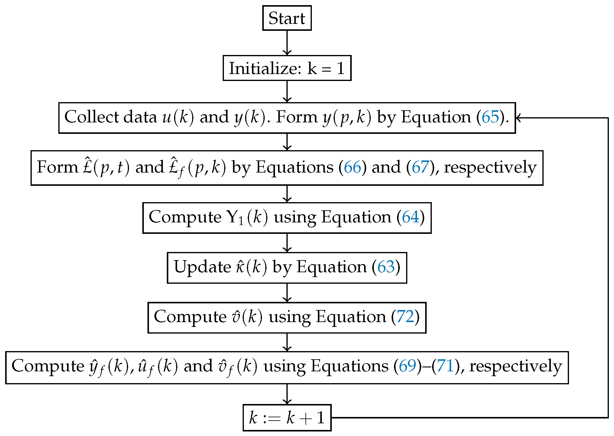
4. The Maximum Likelihood-Based Multi-Innovation Stochastic Gradient Algorithm

In this section, the ML-MI-SG algorithm is derived by introducing the theory of maximum likelihood in order to improve the recognition accuracy and convergence rate of the algorithm.

For the provided dataset, $g_N:=[g\left(1\right),g\left(2\right),\dots ,g\left(N\right)]$ and ${\varrho }_N:=[\varrho \left(1\right),\varrho \left(2\right),\dots ,\varrho \left(N\right)]$, and the likelihood function $F(g_N|{\varrho }_{N-1},\kappa )$ is identical to $f(g_N|{\varrho }_{N-1},\kappa )$. $\varrho \left(k\right),g\left(k\right)$ and $\kappa$ are not correlated with $v\left(k\right)$. The $g_N$, ${\varrho }_N$ and $\kappa$ can be represented as

$$\begin{array}{cc}\hfill & F(g_N|{\varrho }_{N-1},\kappa )=f(g_N|{\varrho }_{N-1},\kappa )\hfill \\ \hfill & =f(y\left(N\right)|g_{N-1},{\varrho }_{N-1},\kappa )f(g(N-1)|g_{N-2},{\varrho }_{N-2},\kappa ),\dots ,f(g\left(1\right)|g\left(0\right),\varrho \left(0\right),\kappa )\hfill \\ \hfill & =\prod _{k=1}^{N}f(g\left(k\right)|g(k-1),\varrho (k-1),\kappa )\hfill \\ \hfill & =\prod _{k=1}^{N}f({\zeta }^T\left(k\right)\kappa +v\left(k\right)|g(k-1),\varrho (k-1),\kappa )\hfill \\ \hfill & =\frac{1}{{\left(2\pi {\sigma }^2\right)}^{\frac{N}{2}}}exp\left(-\frac{1}{2{\sigma }^2}\sum _{k=1}^N{v}^2\left(k\right)\right)+\rho ,\hfill \end{array}$$

(40)

which $\rho$ as constant. The algorithm is acquired through optimizing the $F(g_N|{\varrho }_{N-1},\kappa )$, which signifies,

$$\begin{array}{c}\hfill \widehat{\kappa }=ar{g}_{\kappa }maxF(g_N|{\varrho }_{N-1},\kappa ).\end{array}$$

(41)

From Equation (40), defining $f(g_N|{\varrho }_{N-1},\kappa )$ as a log-likelihood function,

$$\begin{array}{cc}\hfill & k(g_N|{\varrho }_{N-1},\kappa ):=lnf(g_N|{\varrho }_{N-1},\kappa )=ln\eta -\frac{N}{2}ln2\pi -\frac{N}{2}ln{\sigma }^2-\frac{1}{2{\sigma }^2}\sum _{k=1}^N{v}^2\left(k\right).\hfill \end{array}$$

(42)

where $\eta$ is a constant that can be obtained from observations up to moment k. Maximum likelihood estimation of the noise variance ${\sigma }^2$ leads to the function $k(g_N|{\varrho }_{N-1},\kappa )$ = max. Setting $f(g_N|{\varrho }_{N-1},\kappa )$ to zero produces

$$\begin{array}{c}\hfill \frac{\partial k(g_N|{\varrho }_{N-1},\kappa )}{\partial {\sigma }^2}{|}_{{\widehat{\sigma }}^2}=0,\end{array}$$

(43)

where the value of ${\widehat{\sigma }}^2$ is determined by

$$\begin{array}{c}\hfill {\widehat{\sigma }}^2=\frac{1}{N}\sum _{k=1}^N{v}^2\left(k\right).\end{array}$$

(44)

Substituting Equation (44) into Equation (42) yields

$$\begin{array}{cc}\hfill k(g_N|{\varrho }_{N-1},\kappa )& =ln\eta -\frac{N}{2}(1+ln2\pi )-\frac{N}{2}ln\left[\frac{1}{N}\sum _{k=1}^N{v}^2\left(k\right)\right]\hfill \\ \hfill & ={\rho }_1-\frac{N}{2}ln\left[\frac{1}{N}\sum _{k=1}^N{v}^2\left(k\right)\right],\hfill \end{array}$$

(45)

where ${\rho }_1=ln\eta -\frac{N}{2}ln2\pi -\frac{N}{2}$.

From Equation (45), the maximum value of $k(g_N|{\varrho }_{N-1},\kappa ){|}_{\widehat{\kappa }}$ can be obtained by minimizing the objective function

$$\begin{array}{c}\hfill {\Delta }_2\left(\widehat{\kappa }\right):=\frac{1}{2}\sum _{k=1}^N{v}^2\left(k\right){|}_{\widehat{\kappa }},\end{array}$$

(46)

where

$$\begin{array}{c}\hfill v\left(k\right)=\frac{1}{C_1\left(z^{-1}\right)}[A_{\alpha }\left(z^{-1}\right)y\left(k\right)-B_{\alpha }\left(z^{-1}\right)u\left(k\right)].\end{array}$$

(47)

Therefore, to obtain the $\widehat{\kappa }$ of the ARMAX model, the objective function ${\Delta }_2\left(\widehat{\kappa }\right)$ must be minimized.

Using the estimated parameter $\widehat{\kappa }$ to construct the estimates of $C_1\left(z\right)$ at a particular time t:

$$\begin{array}{c}\hfill {\widehat{C}}_1(k,z):=1+\widehat{c_1}\left(k\right)z^{-1}+\widehat{c_2}\left(k\right)z^{-2}+\widehat{c_3}\left(k\right)z^{-3}+\widehat{c_4}\left(k\right)z^{-4}.\end{array}$$

(48)

Applying the gradient search, minimizing Equation (46) yields the desired result.

$$\begin{array}{c}\hfill \widehat{\kappa }\left(k\right)=\widehat{\kappa }(k-1)-{\Lambda }_1\left(k\right)\mathrm{grad}\left[{\Delta }_2\left(\kappa (k-1)\right)\right],\end{array}$$

(49)

where ${\Lambda }_1\left(k\right)$ as convergence factor. Equation (46) expresses the cost function as follows:

$$\begin{array}{c}\hfill {\Delta }_2\left(\kappa \left(k\right)\right)={\Delta }_2\left(\kappa (k-1)\right)+\frac{1}{2}{v}^2\left(k\right).\end{array}$$

(50)

Define ${\Xi }_f{\left(k\right):=-(\partial v\left(k\right)/\partial \kappa )|}_{\widehat{\kappa }(k-1)}$. ${\Delta }_2\left(\kappa (k-1)\right)$ can be rewritten as

$$\begin{array}{c}\hfill \mathrm{grad}\left[{\Delta }_2(\kappa (k-1),k)\right]=\mathrm{grad}\left[{\Delta }_2(\kappa (k-1),k-1)\right]+{\Xi }_f{\left(k\right)v\left(k\right)|}_{\widehat{\kappa }(k-1)}.\end{array}$$

(51)

The approximation of the gradient would be

$$\begin{array}{c}\hfill \mathrm{grad}\left[{\Delta }_2(\kappa (k-1),k)\right]={\Xi }_f{\left(k\right)v\left(k\right)|}_{\widehat{\kappa }(k-1)}.\end{array}$$

(52)

Here, ${\Lambda }_1\left(k\right)$ is chosen in the following manner:

$$\begin{array}{c}\hfill {\Lambda }_1\left(k\right)=\frac{1}{{{\rm Y}}_1\left(k\right)},{{\rm Y}}_1\left(k\right)={\lambda }_1{{\rm Y}}_1(k-1)+{\Vert {\Xi }_f\left(k\right)\Vert }^2.\end{array}$$

(53)

Calculating $v{\left(k\right)}^{\prime }s$ partial derivative in (47), the $a_j,b_j$, and $c_j$ at the point $\widehat{\kappa }(k-1)$ gives

$$\begin{array}{cc}\hfill \frac{\partial v\left(k\right)}{\partial {\tau }_s}{|}_{\widehat{\kappa }(k-1)}=& [\frac{\partial v\left(k\right)}{\partial a_1},\frac{\partial v\left(k\right)}{\partial a_2},\frac{\partial v\left(k\right)}{\partial a_3},\frac{\partial v\left(k\right)}{\partial a_4},\frac{\partial v\left(k\right)}{\partial b_1},\frac{\partial v\left(k\right)}{\partial b_2},\frac{\partial v\left(k\right)}{\partial b_3}]\hfill \\ \hfill =& [\frac{z^{-1}\widehat{y}\left(k\right)}{\widehat{T}(k-1,z)},\frac{z^{-2}\widehat{y}\left(k\right)}{\widehat{T}(k-1,z)},\frac{z^{-3}\widehat{y}\left(k\right)}{\widehat{T}(k-1,z)},\frac{z^{-4}\widehat{y}\left(k\right)}{\widehat{T}(k-1,z)},\hfill \\ \hfill & \frac{z^{-1}\widehat{u}\left(k\right)}{\widehat{T}(k-1,z)},\frac{z^{-2}\widehat{u}\left(k\right)}{\widehat{T}(k-1,z)},\frac{z^{-3}\widehat{u}\left(k\right)}{\widehat{T}(k-1,z)}]\hfill \\ \hfill =& [{\widehat{y}}_f(k-1),{\widehat{y}}_f(k-2),{\widehat{y}}_f(k-3),{\widehat{y}}_f(k-4),\hfill \\ \hfill & {\widehat{u}}_f(k-1),{\widehat{u}}_f(k-2),{\widehat{u}}_f(k-3)],\hfill \end{array}$$

(54)

$$\begin{array}{cc}\hfill \frac{\partial v\left(k\right)}{\partial {\tau }_n}{|}_{\widehat{\kappa }(k-1)}=& [\frac{\partial v\left(k\right)}{\partial c_1},\frac{\partial v\left(k\right)}{\partial c_2},\frac{\partial v\left(k\right)}{\partial c_3},\frac{\partial v\left(k\right)}{\partial c_4}]\hfill \\ \hfill =& [\frac{z^{-1}\widehat{v}\left(k\right)}{\widehat{T}(k-1,z)},\frac{z^{-2}\widehat{v}\left(k\right)}{\widehat{T}(k-1,z)},\frac{z^{-3}\widehat{v}\left(k\right)}{\widehat{T}(k-1,z)},\frac{z^{-4}\widehat{v}\left(k\right)}{\widehat{T}(k-1,z)}\hfill \\ \hfill =& [-{\widehat{v}}_f(k-1),-{\widehat{v}}_f(k-2),-{\widehat{v}}_f(k-3),-{\widehat{v}}_f(k-4)],\hfill \end{array}$$

(55)

where ${\widehat{y}}_f\left(k\right),{\widehat{u}}_f$, and ${\widehat{v}}_f\left(k\right)$ are defined as

$$\begin{array}{c}\hfill {\widehat{y}}_f\left(k\right):=\frac{\widehat{y}\left(k\right)}{\widehat{T}(k-1,z)}=\widehat{y}\left(k\right)-\sum _{i=1}^4{\widehat{c}}_i(k-1){\widehat{y}}_f(k-i),\end{array}$$

(56)

$$\begin{array}{c}\hfill {\widehat{u}}_f\left(k\right):=\frac{\widehat{u}\left(k\right)}{\widehat{T}(k-1,z)}=\widehat{u}\left(k\right)-\sum _{i=1}^4{\widehat{c}}_i(k-1){\widehat{u}}_f(k-i),\end{array}$$

(57)

$$\begin{array}{c}\hfill {\widehat{v}}_f\left(k\right):=\frac{\widehat{v}\left(k\right)}{\widehat{T}(k-1,z)}=\widehat{v}\left(k\right)-\sum _{i=1}^4{\widehat{c}}_i(k-1){\widehat{v}}_f(k-i).\end{array}$$

(58)

The ${\Xi }_f\left(k\right)$ rewritten as

$$\begin{array}{cc}\hfill {\Xi }_f\left(k\right):=-& \frac{\partial v\left(k\right)}{\partial \tau }{|}_{\widehat{\kappa }(k-1)}\hfill \\ \hfill =-& [\frac{\partial v\left(k\right)}{\partial a_1},\frac{\partial v\left(k\right)}{\partial a_2},\frac{\partial v\left(k\right)}{\partial a_3},\frac{\partial v\left(k\right)}{\partial a_4},\frac{\partial v\left(k\right)}{\partial b_1},\frac{\partial v\left(k\right)}{\partial b_2},\frac{\partial v\left(k\right)}{\partial b_3},\hfill \\ \hfill & \frac{\partial v\left(k\right)}{\partial c_1},\frac{\partial v\left(k\right)}{\partial c_2},\frac{\partial v\left(k\right)}{\partial c_3},\frac{\partial v\left(k\right)}{\partial c_4}{]}_{\widehat{\kappa }(k-1)}^T.\hfill \end{array}$$

(59)

The ${\Xi }^T\left(k\right)$ and ${\Xi }_f\left(k\right)$ are expanded into ${\pounds }^T(p,k)$ and ${\pounds }_f^T(p,k)$, where

$$\begin{array}{c}\hfill {\pounds }_f^T(p,k):=[{\Xi }_f\left(k\right),{\Xi }_f(k-1),\cdots ,{\Xi }_f(k-l+1)]\in R^{n_0\times p}.\end{array}$$

(60)

The ML-MI-SG algorithm to estimate $\widehat{\kappa }\left(k\right)$ based on maximum likelihood.

$$\begin{array}{cc}\hfill \widehat{\kappa }\left(k\right)& =\widehat{\kappa }(k-1)+\frac{{\widehat{\Xi }}_f\left(k\right)}{{{\rm Y}}_1\left(k\right)}[\widehat{y}(p,k)-{\widehat{\pounds }}^T(p,k)\widehat{\kappa }(k-1)],\hfill \end{array}$$

(61)

$$\begin{array}{cc}\hfill {{\rm Y}}_1\left(k\right)& ={\lambda }_1{{\rm Y}}_1(k-1)+{\Vert {\widehat{\pounds }}_f(p,k)\Vert }^2.\hfill \end{array}$$

(62)

Then, an ML-MI-SG algorithm may be obtained to estimate the parameter vector $\kappa$.

$$\begin{array}{cc}\hfill \widehat{\kappa }\left(k\right)& =\widehat{\kappa }(k-1)+\frac{{\widehat{\Xi }}_f\left(k\right)}{{{\rm Y}}_1\left(k\right)}[\widehat{y}(p,k)-{\widehat{\pounds }}^T(p,k)\widehat{\kappa }(k-1)],\hfill \end{array}$$

(63)

$$\begin{array}{cc}\hfill {{\rm Y}}_1\left(k\right)& ={\lambda }_1{{\rm Y}}_1(k-1)+{\Vert {\widehat{\pounds }}_f(p,k)\Vert }^2,\hfill \end{array}$$

(64)

$$\begin{array}{cc}\hfill y(p,k)& ={[y\left(k\right),y(k-1),\dots ,y(k-p+1)]}^T,\hfill \end{array}$$

(65)

$$\begin{array}{cc}\hfill \widehat{\pounds }(p,k):& =[\widehat{\Xi }\left(k\right),\widehat{\Xi }(k-1),\dots ,\widehat{\Xi }(k-l+1)],\hfill \end{array}$$

(66)

$$\begin{array}{cc}\hfill {\widehat{\pounds }}_f(p,k):& =[{\widehat{\Xi }}_f\left(k\right),{\widehat{\Xi }}_f(k-1),\dots ,{\widehat{\Xi }}_f(k-l+1)],\hfill \\ \hfill {\widehat{\Xi }}_f\left(k\right):& =[-{\widehat{y}}_f(k-1),-{\widehat{y}}_f(k-2),-{\widehat{y}}_f(k-3),-{\widehat{y}}_f(k-4),\hfill \\ \hfill & -{\widehat{u}}_f(k-1),-{\widehat{u}}_f(k-2),-{\widehat{u}}_f(k-3),\hfill \end{array}$$

(67)

$$\begin{array}{cc}\hfill & {\widehat{v}}_f(k-1),{\widehat{v}}_f(k-2),{\widehat{v}}_f(k-3),{\widehat{v}}_f(k-4)]\hfill \end{array}$$

(68)

$$\begin{array}{cc}\hfill {\widehat{y}}_f\left(k\right):& =\frac{\widehat{y}\left(k\right)}{\widehat{T}(k-1,z)}=\widehat{y}\left(k\right)-\sum _{i=1}^4{\widehat{c}}_i(k-1){\widehat{y}}_f(k-i),\hfill \end{array}$$

(69)

$$\begin{array}{cc}\hfill {\widehat{u}}_f\left(k\right):& =\frac{\widehat{u}\left(k\right)}{\widehat{T}(k-1,z)}=\widehat{u}\left(k\right)-\sum _{i=1}^4{\widehat{c}}_i(k-1){\widehat{u}}_f(k-i),\hfill \end{array}$$

(70)

$$\begin{array}{cc}\hfill {\widehat{v}}_f\left(k\right):& =\frac{\widehat{v}\left(k\right)}{\widehat{T}(k-1,z)}=\widehat{v}\left(k\right)-\sum _{i=1}^4{\widehat{c}}_i(k-1){\widehat{v}}_f(k-i).\hfill \end{array}$$

(71)

$$\begin{array}{cc}\hfill \widehat{v}\left(k\right)& =y\left(k\right)-{\widehat{\Xi }}^T\left(k\right)\widehat{\kappa }\left(k\right).\hfill \end{array}$$

(72)

The proposed algorithms in this paper can combine other parameter estimation algorithms [97,98,99,100,101,102] to study new parameter identification approaches of different systems [103,104,105,106,107] and can be applied to other fields. To start the ML-MI-SG algorithm, set the initial values $\widehat{\kappa }\left(0\right)=I_{n_0}/l$, ${{\rm Y}}_1\left(0\right)=1,{\lambda }_1=0.99,{\widehat{y}}_f\left(k\right)=1/l,{\widehat{u}}_f\left(k\right)=1/l,{\widehat{v}}_f\left(k\right)=1/l,\widehat{v}\left(k\right)=1/l$, with $i\le 0$ and $l={10}^6$. The identification process for computing $\widehat{\kappa }\left(k\right)$ with the ML-MI-SG algorithm is presented in Figure 3.

5. Wave Peak Frequency and Ship Motion Parameter Calculation

Based on Section 2, the ship motion parameter and wave peak frequency can be calculated from Equation (21), where

$$\begin{array}{c}\hfill \tau :=[{\widehat{\tau }}_s\left(k\right),{\widehat{\tau }}_{nf}\left(k\right)]=[a_1,a_2,a_3,a_4,b_1,b_2,b_3,c_1,c_2,c_3,c_4],\end{array}$$

(73)

where

$$\tau \left(11\right)=c_4=\frac{h-T}{T},\tau \left(5\right)=b_1=\frac{K{h}^2}{T},\tau \left(1\right)=a_1=\frac{4T-h-2\zeta {\omega }_{n}hT}{T}.$$

Thus, the parameters K and T and the wave peak frequency ${\omega }_n$ can be acquired using the following equations:

$$\begin{array}{c}\hfill T=\frac{h}{\tau \left(11\right)+1},K=\frac{\tau \left(5\right)T}{h^2},{\omega }_n=\frac{4T-\tau \left(1\right)T-h}{2\zeta hT}.\end{array}$$

(74)

6. Simulation Results and Analysis

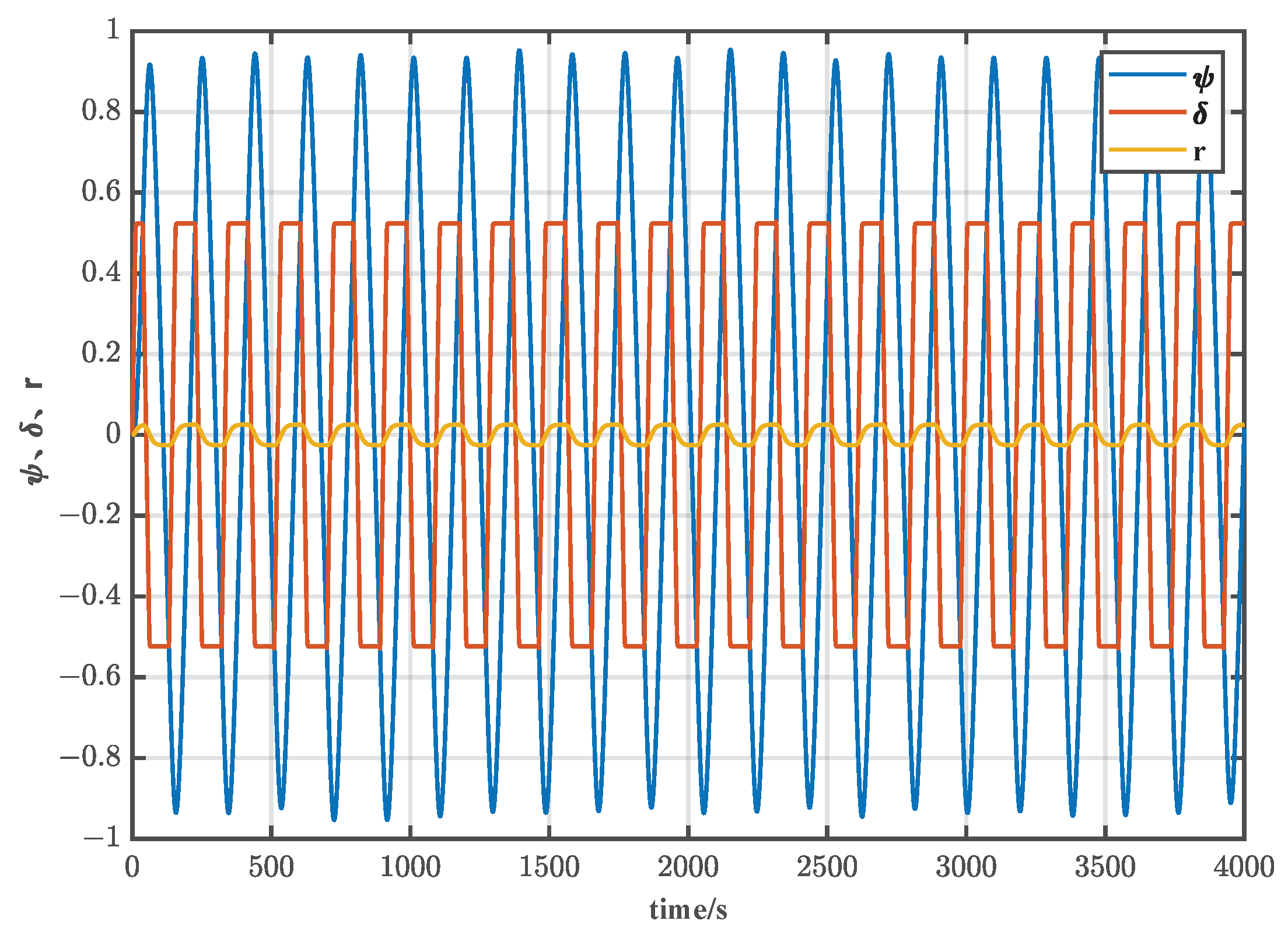
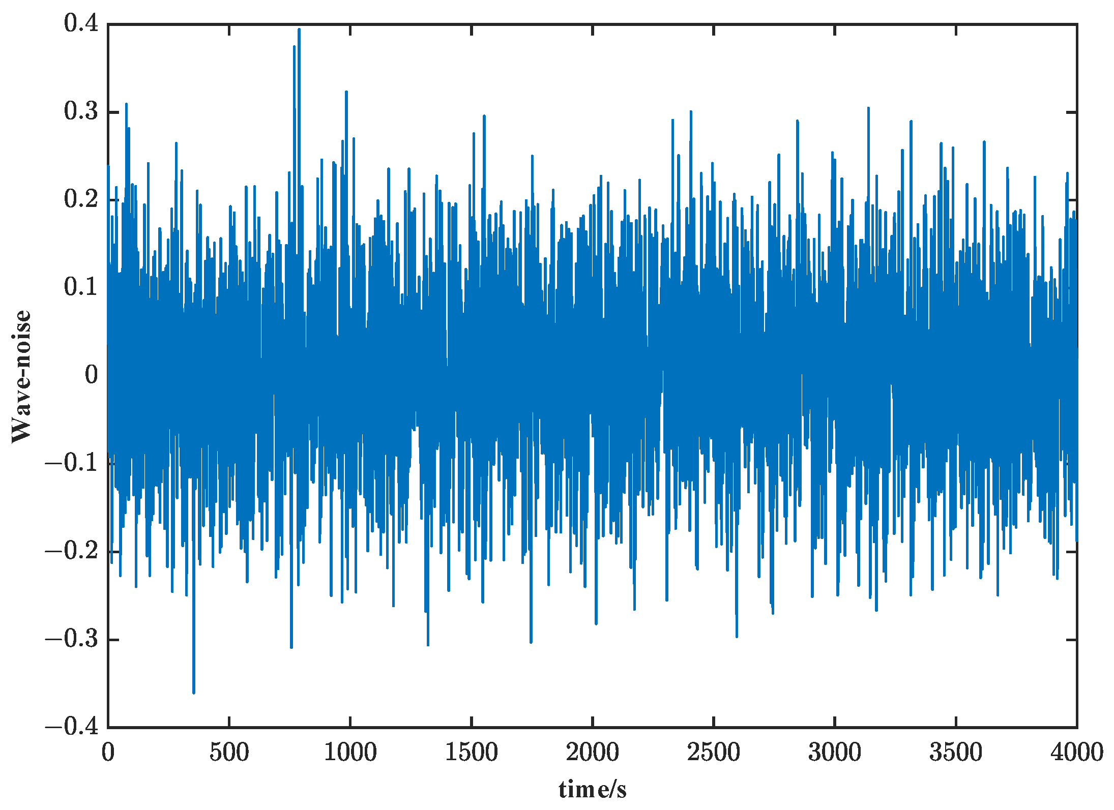
6.1. Identification Input Design

To confirm the efficacy of the ML-MI-SG algorithm, a standard ship model is used instead of the ship’s motion in second-order waves. Subsequently, the simulation model’s parameters were identified separately using the MI-SG and ML-MI-SG algorithms.

The mathematical model of the vessel is anchored in the Nomoto model which has been expounded in Equation (8). The specifications of the vessel needed for establishing the Nomoto model have been rendered in

Table 1. Detailed parameters of Yu Peng.

Length between perpendiculars L (m)	189.0
Breadth (molded) B (m)	$27.8$
Designed draft D (m)	$11.0$
Volume of displacement ∇ (m${}^3$)	42,293.0
Block coefficient $C_b$	$0.72$
Trial speed V (kn)	$17.3$
Rudder area $A_R$ (m${}^2$)	38
Longitudinal center of gravity $x_c$ (m)	$-1.8$

. The precise values of the Nomoto model parameters for Yu Peng were derived using Visual Basic from the particulars relating to Yu Peng presented in Table 1 ([43]). The obtained values have been depicted in

Table 2. Mathematical model parameters for Yu Peng.

Turning ability index K (1/s)	0.38
Following index T (s)	$297.75$
$\alpha$	$11.95$
$\beta$	23,928.91

. A simulation of the 30 Z-shaped maneuvers was carried out utilizing the fourth-order Runge–Kutta method. Subsequently, data on the rudder angle and heading angle were collected and presented in Figure 4.

Remark 1.

Yu Peng  is a new type of teaching and training ship at Dalian Maritime University, which is a collection of modern ship design, manufacturing and equipment technology, advanced design; is well-equipped with a large number of the world’s most intelligent and advanced, highly efficient and environmentally friendly equipment, which is mainly used for teaching internships for students of nautical majors; and is applicable to the loading of bulk and general cargoes, major complete sets of project equipment and containers, as well as scientific research and experiments in disciplines such as traffic information engineering and control, navigation science and technology, engine engineering, and environmental engineering, etc., and has been tested with sufficient data. Therefore, the data are relatively complete and help to validate the identification of ship modeling parameters.

The ship’s rudder system consists of a control drive, a servo motor, a reduction drive, and a sensor. Currently, large ships mostly use hydraulic servos to steer the ship. The hydraulic rudder is a hydraulic servo system with variable parameters and variable load. Without load, the rudder system can be regarded as a first-order inertial link, and the true rudder angle $\delta$ is similar to a square wave considering the saturation effect of the rudder and the dynamic characteristics. Therefore, it is assumed that the simulated data generated using the first-order Nomoto model coincide with the actual ship motion and can therefore be used as real data for model parameter identification purposes.

Wave disturbance is primarily considered for the effect of second-order wave disturbance force. This paper employs a variance of ${\sigma }^2=0.01$ and a sampling time of $t=1$ s with Gaussian white noise, as illustrated in Figure 5.

Remark 2.

The input used in this paper is Gaussian white noise, which is an implicit model for unknown external perturbations. When the assumed input–output order exceeds a certain minimum value, the perturbation information will be completely absorbed into the identified model coefficients, which has little effect on the identification of parameters. Because Gaussian white noise can reflect the noise situation in the actual communication channel, it can reflect some characteristics of channel noise more realistically, and it can be expressed by specific mathematical expressions, which is suitable for analyzing and calculating the system’s anti-noise performance, and it is widely used in theoretical analysis of communication systems.

Remark 3.

The PM spectrum ([71]) is introduced to analyze the variation in the peak frequency of waves under different sea states. The PM spectrum is written:

$$\begin{array}{c}\hfill S\left(w\right)=A{w}^{-5}exp(-B{w}^{-4})\end{array}$$

(75)

where $A=8.1\times {10}^{-3}{g}^2$, $B=0.74\times {\left(\frac{g}{V_s}\right)}^4$, $V_s$ is the wind speed, and g is the gravity constant. Assuming that waves can be represented as Gaussian random processes and that S(w) is narrow-banded, the PM spectrum can be reformulated in terms of significant wave height:

$$\begin{array}{cc}\hfill A& =8.1\times {10}^{-3}{g}^2,\hfill \end{array}$$

(76)

$$\begin{array}{cc}\hfill B& =0.0323\times {\left(\frac{g}{V_s}\right)}^2=\frac{3.11}{H_s^2}.\hfill \end{array}$$

(77)

This implies that there is a relationship between wind speed $V_s$ and significant wave height $H_s$ and wave peak frequency $w_0$ as

$$\begin{array}{c}\hfill H_s=0.21\times \frac{V^2}{g},\end{array}$$

(78)

$$\begin{array}{c}\hfill w=0.4\times \sqrt{\frac{g}{H_s}}.\end{array}$$

(79)

The PM spectra at different values of $H_s$ are shown in Figure 6. From Figure 6, it can be seen that as the degree of the sea state increases, the wave peak frequency will decrease. In order to verify the effect of the proposed algorithm, the following section will identify the wave peak frequency with different sea states.

6.2. Parameter Identification Experiments

Built on the data that were gathered, the parameters of the ship motion model were established through employment of the ML-MI-SG algorithm at innovation lengths ($p=1,2,3$). It is important to note that it is similar to the ML-SG algorithm in that the innovation length $p=1$. To ascertain algorithm efficacy for identification at ${\omega }_n=0.4$, we identified model parameters using Equations (63)–(72) of the ML-MI-SG algorithm and the aforementioned Z-type test data to validate Equation (21). To assess the recognition algorithm’s online capabilities, the recognition time was an extension of 4000 s. At $t=2000$ s, the ship speed of the unmanned ship was varied so that the K-T parameter of the ship was changed, and the identification results obtained were compared.

The following figure compares the wave frequency estimation ${\omega }_n$, the ship motion parameter estimation K,T, the error estimation accuracy $\delta$ for the same ${\omega }_0$, the MI-SG algorithm and the ML-MI-SG algorithm under the same innovation length, and the ML-MI-SG algorithm under different innovation lengths, where $\delta :=\left|\right|\widehat{\tau }\left(k\right)-\tau \left(k\right)\left|\right|/\left|\right|\tau \left(k\right)\left|\right|$.

The results of the simulation depicted in Figure 7, Figure 8 and Figure 9 demonstrate the accurate estimation of ship K-T parameters and wave peak frequency by both the MI-SG and ML-MI-SG algorithms. To confirm the superiority of the ML-MI-SG algorithm, its performance is compared to that of the MI-SG algorithm under the condition of an innovation length of $p=2$. To examine the impact of various innovation lengths on the algorithms, the performance at different innovation lengths is compared. The findings from Table 3 and Table 4 and Figure 7, Figure 8 and Figure 9 indicate the following outcomes.

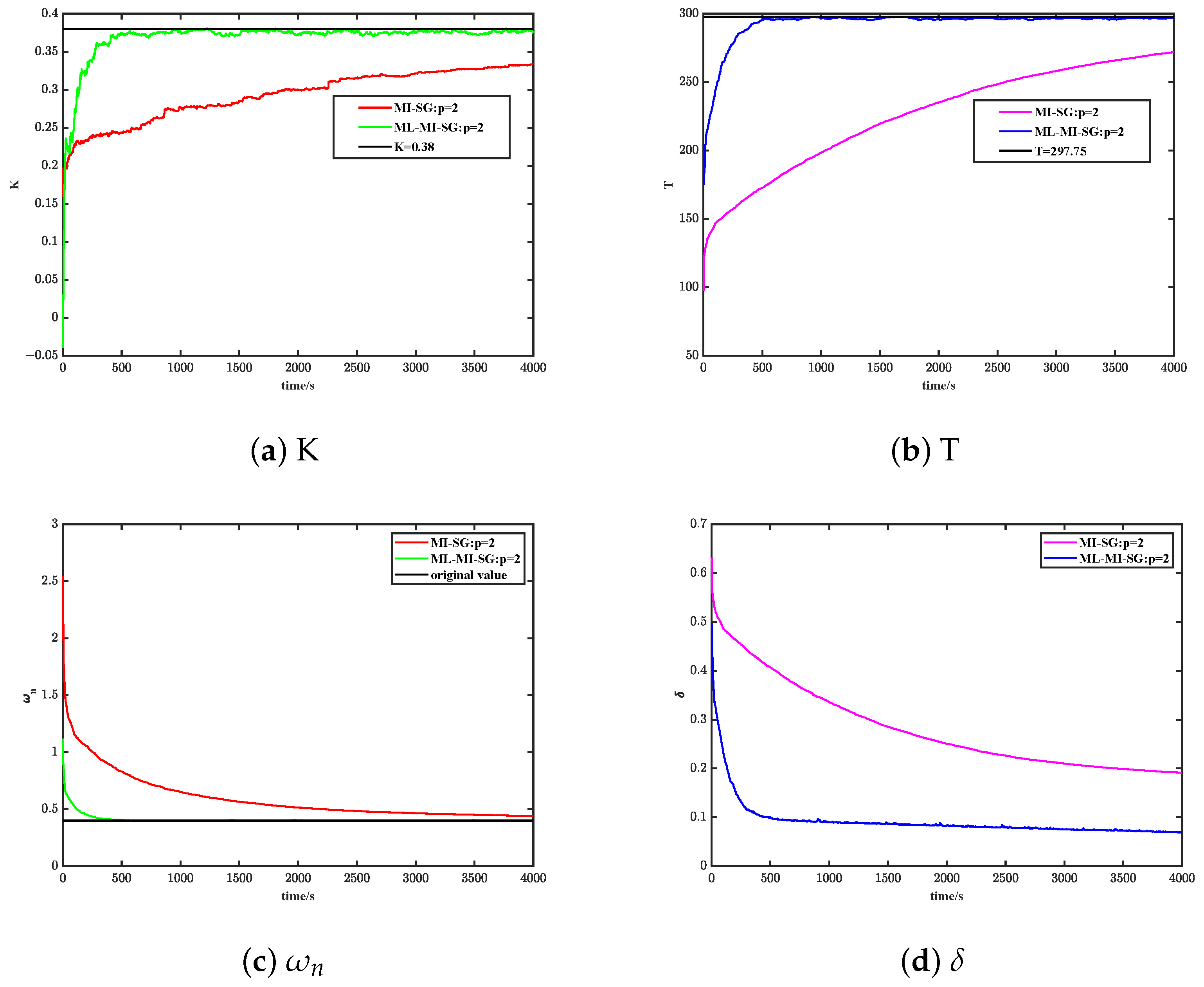
• The estimation errors of both the MI-SG algorithm and the ML-MI-SG algorithm decrease over time. Please refer to Figure 7. The ML-MI-SG algorithm demonstrates superior convergence speed and identification accuracy when compared with the MI-SG algorithm, enabling it to more effectively identify and obtain the parameters of the ship–wave model, as depicted in Figure 7.
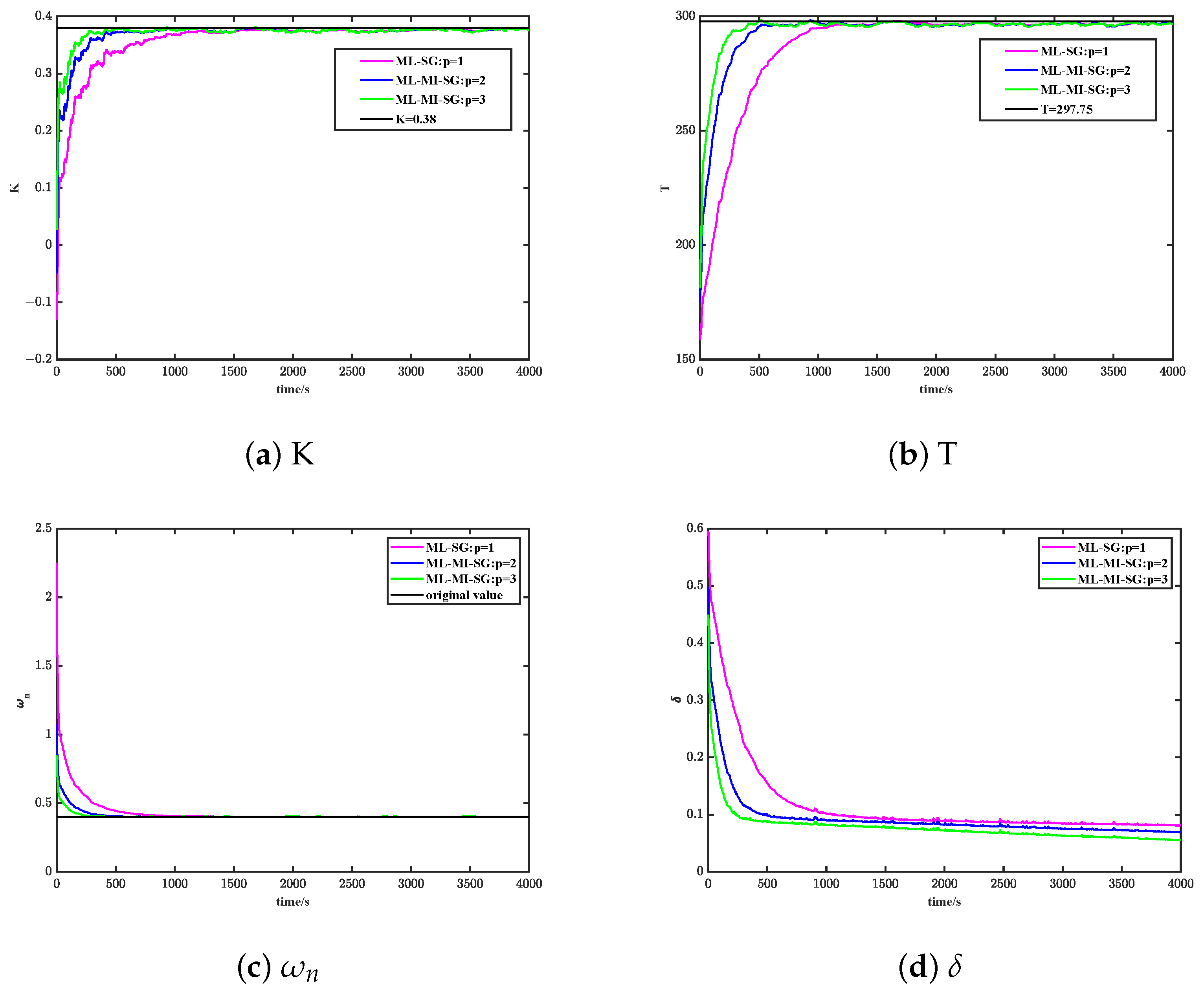
• In the case of the same innovation length p, the convergence speed and recognition accuracy of the ML-MI-SG algorithm are better than that of the MI-SG algorithm; by means of the control variable method, comparing the ML-MI-SG algorithms with different innovation lengths p in the case of the other states being the same, the convergence speed and the recognition accuracy are directly proportional to the change of the innovation length p, as illustrated by Table 3 and Table 4 and Figure 8.
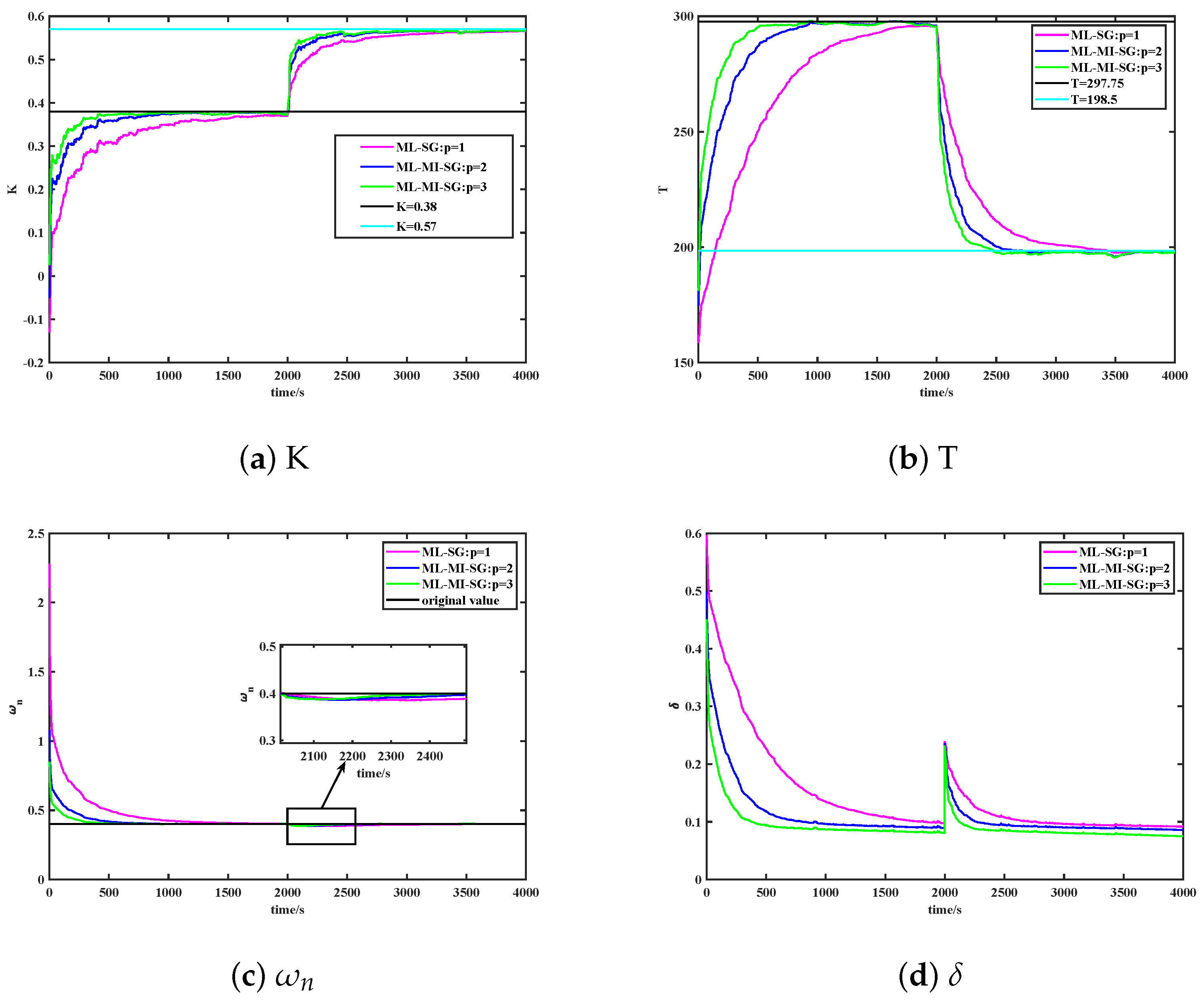
• For ship state changes, the ML-MI-SG algorithm is able to respond quickly to K and T parameter changes due to ship speed and load changes and accurately identify the new K and T parameters of the ship in a short period of time, showing excellent real-time performance, as depicted in Figure 9.

Figure 7. Identification results for comparing MI-SG and ML-MI-SG algorithms at a different innovation length of p = 2.

Figure 7. Identification results for comparing MI-SG and ML-MI-SG algorithms at a different innovation length of p = 2.

Figure 8. Identification results of each parameter for different innovation lengths.

Figure 8. Identification results of each parameter for different innovation lengths.

Figure 9. Identification results when K and T parameters are varied for different innovation lengths.

Figure 9. Identification results when K and T parameters are varied for different innovation lengths.

Table 3. Comparison of K and T parameter identification of ML-MI-SG algorithm with different innovation lengths.

K	ML-MI-SG			T	ML-MI-SG
time/s	p = 1	p = 2	p = 3	time/s	p = 1	p = 2	p = 3
100	0.18729	0.27794	0.32097	100	199.25624	244.77772	268.22143
200	0.25862	0.32483	0.35365	200	225.48425	271.49848	287.99145
500	0.33842	0.37251	0.37825	500	274.01053	295.54320	295.77890
1000	0.36728	0.37637	0.37624	1000	294.89304	296.94850	296.48548
2000	0.37371	0.37306	0.37267	2000	296.40574	295.71300	295.67858
4000	0.37648	0.37602	0.37574	4000	296.91472	296.97271	296.99007
true value	0.38	0.38	0.38	true value	297.75	297.75	297.75

Table 3. Comparison of K and T parameter identification of ML-MI-SG algorithm with different innovation lengths.

K	ML-MI-SG			T	ML-MI-SG
time/s	p = 1	p = 2	p = 3	time/s	p = 1	p = 2	p = 3
100	0.18729	0.27794	0.32097	100	199.25624	244.77772	268.22143
200	0.25862	0.32483	0.35365	200	225.48425	271.49848	287.99145
500	0.33842	0.37251	0.37825	500	274.01053	295.54320	295.77890
1000	0.36728	0.37637	0.37624	1000	294.89304	296.94850	296.48548
2000	0.37371	0.37306	0.37267	2000	296.40574	295.71300	295.67858
4000	0.37648	0.37602	0.37574	4000	296.91472	296.97271	296.99007
true value	0.38	0.38	0.38	true value	297.75	297.75	297.75

Table 4. Comparison of ${\omega }_n$ and $\delta$ parameter identification of ML-MI-SG algorithm with different innovation lengths.

${\mathit{\omega }}_{\mathit{n}}$	ML-MI-SG			$\mathit{\delta }$	ML-MI-SG
time/s	p = 1	p = 2	p = 3	time/s	p = 1	p = 2	p = 3
100	1.06125	0.62012	0.51603	100	0.38632	0.23137	0.15548
200	0.75940	0.50463	0.44432	200	0.29932	0.15322	0.10550
500	0.49931	0.41674	0.40427	500	0.15572	0.09959	0.08865
1000	0.42119	0.40333	0.40288	1000	0.10179	0.08994	0.08179
2000	0.40430	0.40423	0.40258	2000	0.08874	0.08240	0.07207
4000	0.40244	0.40229	0.40118	4000	0.08081	0.06918	0.05526
true value	0.4	0.4	0.4

Table 4. Comparison of ${\omega }_n$ and $\delta$ parameter identification of ML-MI-SG algorithm with different innovation lengths.

${\mathit{\omega }}_{\mathit{n}}$	ML-MI-SG			$\mathit{\delta }$	ML-MI-SG
time/s	p = 1	p = 2	p = 3	time/s	p = 1	p = 2	p = 3
100	1.06125	0.62012	0.51603	100	0.38632	0.23137	0.15548
200	0.75940	0.50463	0.44432	200	0.29932	0.15322	0.10550
500	0.49931	0.41674	0.40427	500	0.15572	0.09959	0.08865
1000	0.42119	0.40333	0.40288	1000	0.10179	0.08994	0.08179
2000	0.40430	0.40423	0.40258	2000	0.08874	0.08240	0.07207
4000	0.40244	0.40229	0.40118	4000	0.08081	0.06918	0.05526
true value	0.4	0.4	0.4

7. Conclusions

The paper presents a novel ship–wave model parameter identification algorithm based on the maximum likelihood multi-innovation stochastic gradient. The algorithm combines the essence of maximum likelihood and multi-innovation theory. The following conclusions can be drawn based on simulations and comparisons.

• Typically, traditional methods require a large amount of test data to produce reliable parameter estimation results, while the system identification method can achieve reliable parameter estimation with less test data; secondly, the data error is about 5%, which effectively reduces the data error and improves the accuracy of parameter estimation.
• Compared with the MI-SG algorithm, the ML-MI-SG algorithm exhibits higher accuracy in parameter identification, with an improvement of about 10%. The ML-MI-SG algorithm combines the key ideas of maximum likelihood and multi-innovation theory, and further improves the accuracy of parameter identification through the introduction of maximum likelihood estimation methods.
• Additionally, the ML-MI-SG algorithm converges much faster than the MI-SG algorithm. The discrimination curve is also smoother with a smaller fluctuation range, resulting in better parameter acquisition performance for designing controllers and observers and other related tasks.

The ML-MI-SG algorithm presented in this paper is expected to offer a dependable solution to the issue of identifying the parameters of ship–wave models. This will promote research and applications in the related fields. With less test data, the proposed algorithm can provide reliable parameter estimation. It can be used to obtain model parameters in aerospace, robotics, artificial intelligence, industrial processes, and other fields in order to build accurate research models. Future research can predict ship maneuverability based on the parameters obtained from system identification algorithms [108,109,110,111]. Intelligent algorithms can be introduced to further improve identification results and advance related technologies and applications.

References

1. Handayani, M.P.; Melia, P.; Kim, H.; Lee, S.; Lee, J. Navigating Energy Efficiency: A Multifaceted Interpretability of Fuel Oil Consumption Prediction in Cargo Container Vessel Considering the Operational and Environmental Factors. J. Mar. Sci. Eng. 2023, 11, 2165. [Google Scholar] [CrossRef]
2. Niu, Y.; Zhu, F.; Wei, M.; Du, Y.; Zhai, P. A Multi-Ship Collision Avoidance Algorithm Using Data-Driven Multi-Agent Deep Reinforcement Learning. J. Mar. Sci. Eng. 2023, 11, 2101. [Google Scholar] [CrossRef]
3. Ouyang, Z.; Zou, Z.; Zou, L. Nonparametric Modeling and Control of Ship Steering Motion Based on Local Gaussian Process Regression. J. Mar. Sci. Eng. 2023, 11, 2161. [Google Scholar] [CrossRef]
4. Shi, X.; Chen, P.; Chen, L. An Integrated Method for Ship Heading Control Using Motion Model Prediction and Fractional Order Proportion Integration Differentiation Controller. J. Mar. Sci. Eng. 2023, 11, 2294. [Google Scholar] [CrossRef]
5. Grlj, C.; Degiuli, N.; Tuković, Ž.; Farkas, A.; Martić, I. The effect of loading conditions and ship speed on the wind and air resistance of a containership. Ocean Eng. 2023, 273, 113991. [Google Scholar] [CrossRef]
6. Himaya, A.; Sano, M.; Suzuki, T.; Shirai, M.; Hirata, N.; Matsuda, A.; Yasukawa, H. Effect of the loading conditions on the maneuverability of a container ship. Ocean Eng. 2022, 247, 109964. [Google Scholar] [CrossRef]
7. Wall, A.; Thornhill, E.; Barber, H.; McTavish, S.; Lee, R. Experimental investigations into the effect of at-sea conditions on ship airwake characteristics. J. Wind Eng. Ind. Aerodyn. 2022, 223, 104933. [Google Scholar] [CrossRef]
8. Park, D.; Lee, J.; Jung, Y.; Lee, J.; Kim, Y.; Gerhardt, F. Experimental and numerical studies on added resistance of ship in oblique sea conditions. Ocean Eng. 2019, 186, 106070. [Google Scholar] [CrossRef]
9. Perrault, D. Probability of sea condition for ship strength, stability, and motion studies. J. Ship Res. 2021, 65, 1–14. [Google Scholar] [CrossRef]
10. Wang, Z.; Soares, C.; Zou, Z. Optimal design of excitation signal for identification of nonlinear ship manoeuvring model. Ocean Eng. 2020, 196, 106778. [Google Scholar] [CrossRef]
11. Sutulo, S.; Guedes Soares, C. Offline system identification of ship manoeuvring mathematical models with a global optimization algorithm. In Proceedings of the MARSIM 2015: International Conference on Ship Manoeuvrability and Maritime Simulation, Newcastle upon Tyne, UK, 8–11 September 2015; pp. 8–11. [Google Scholar]
12. Skjetne, R.; Fossen, T.; Kokotović, P. Adaptive maneuvering, with experiments, for a model ship in a marine control laboratory. Automatica 2005, 41, 289–298. [Google Scholar] [CrossRef]
13. Sutulo, S.; Guedes Soares, C. Mathematical models for simulation of manoeuvring performance of ships. In Marine Technology and Engineering; Taylor & Francis Group: London, UK, 2011; pp. 661–698. [Google Scholar]
14. Xu, L. Parameter estimation for nonlinear functions related to system responses. Int. J. Control Autom. Syst. 2023, 21, 1780–1792. [Google Scholar] [CrossRef]
15. Xu, L. Separable Newton recursive estimation method through system responses based on dynamically discrete measurements with increasing data length. Int. J. Control Autom. Syst. 2022, 20, 432–443. [Google Scholar] [CrossRef]
16. Ding, F.; Chen, T. Combined parameter and output estimation of dual-rate systems using an auxiliary model. Automatica 2004, 40, 1739–1748. [Google Scholar] [CrossRef]
17. Ding, F.; Chen, T. Parameter estimation of dual-rate stochastic systems by using an output error method. IEEE Trans. Autom. Control 2005, 50, 1436–1441. [Google Scholar] [CrossRef]
18. Fan, Y.M.; Liu, X.M. Auxiliary model-based multi-innovation recursive identification algorithms for an input nonlinear controlled autoregressive moving average system with variable-gain nonlinearity. Int. J. Adapt. Control Signal Process. 2022, 36, 521–540. [Google Scholar] [CrossRef]
19. Wang, J.; Ji, Y.; Zhang, X. Two-stage gradient-based iterative algorithms for the fractional-order nonlinear systems by using the hierarchical identification principle. Int. J. Adapt. Control Signal Process. 2022, 36, 1778–1796. [Google Scholar] [CrossRef]
20. Sutulo, S.; Soares, C. An algorithm for offline identification of ship manoeuvring mathematical models from free-running tests. Ocean Eng. 2014, 79, 10–25. [Google Scholar] [CrossRef]
21. Ueng, S.; Lin, D.; Liu, C. A ship motion simulation system. Virtual Real. 2008, 12, 65–76. [Google Scholar] [CrossRef]
22. Lin, R.; Kuang, W. A fully nonlinear, dynamically consistent numerical model for solid-body ship motion. i. ship motion with fixed heading. Proc. R. Soc. A Math. Phys. Eng. Sci. 2011, 467, 911–927. [Google Scholar] [CrossRef]
23. Francescutto, A.; Contento, G. Bifurcations in ship rolling: Experimental results and parameter identification technique. Ocean Eng. 1999, 26, 1095–1123. [Google Scholar] [CrossRef]
24. Zhang, Z.; Zhang, Y.; Wang, J.; Wang, H. Parameter identification and application of ship maneuvering model based on TO-CSA. Ocean Eng. 2022, 266, 113128. [Google Scholar] [CrossRef]
25. Allotta, B.; Costanzi, R.; Pugi, L.; Ridolfi, A. Identification of the main hydrodynamic parameters of Typhoon AUV from a reduced experimental dataset. Ocean Eng. 2018, 147, 77–88. [Google Scholar] [CrossRef]
26. Cardenas, P.; de Barros, E. Estimation of AUV hydrodynamic coefficients using analytical and system identification approaches. IEEE J. Ocean. Eng. 2019, 45, 1157–1176. [Google Scholar] [CrossRef]
27. Luo, W.; Li, X. Measures to diminish the parameter drift in the modeling of ship manoeuvring using system identification. Appl. Ocean. Res. 2017, 67, 9–20. [Google Scholar] [CrossRef]
28. Xue, Y.; Liu, Y.; Ji, C.; Xue, G. Hydrodynamic parameter identification for ship manoeuvring mathematical models using a Bayesian approach. Ocean Eng. 2020, 195, 106612. [Google Scholar] [CrossRef]
29. Ding, F.; Ma, H.; Pan, J.; Yang, E.F. Hierarchical gradient- and least squares-based iterative algorithms for input nonlinear output-error systems using the key term separation. J. Frankl. Inst. 2021, 358, 5113–5135. [Google Scholar] [CrossRef]
30. Hu, C.; Ji, Y.; Ma, C.Q. Joint two-stage multi-innovation recursive least squares parameter and fractional-order estimation algorithm for the fractional-order input nonlinear output-error autoregressive model. Int. J. Adapt. Control Signal Process. 2023, 37, 1650–1670. [Google Scholar] [CrossRef]
31. Zhang, X.; Ding, F. Optimal adaptive filtering algorithm by using the fractional-order derivative. IEEE Signal Process. Lett. 2022, 29, 399–403. [Google Scholar] [CrossRef]
32. Xu, L.; Ding, F.; Yang, E.F. Auxiliary model multiinnovation stochastic gradient parameter estimation methods for nonlinear sandwich systems. Int. J. Robust Nonlinear Control 2021, 31, 148–165. [Google Scholar] [CrossRef]
33. Ji, Y.; Kang, Z. Three-stage forgetting factor stochastic gradient parameter methods for a class of nonlinear systems. Int. J. Robust Nonlinear Control 2021, 31, 971–987. [Google Scholar] [CrossRef]
34. Zhu, M.; Hahn, A.; Wen, Y.; Bolles, A. Parameter identification of ship maneuvering models using recursive least square method based on support vector machines. TransNav Int. J. Mar. Navig. Saf. Sea Transp. 2017, 11, 23–29. [Google Scholar] [CrossRef]
35. Iseki, T. Real-time estimation of the ship manoeuvrable range in wind. Ocean Eng. 2019, 190, 106396. [Google Scholar] [CrossRef]
36. Nomoto, K.; Taguchi, K.; Honda, K.; Hirano, S. On the steering qualities of ships. J. Zosen Kiokai 1956, 1956, 75–82. [Google Scholar] [CrossRef] [PubMed]
37. Ding, F.; Chen, T. Hierarchical least squares identification methods for multivariable systems. IEEE Trans. Autom. Control 2005, 50, 397–402. [Google Scholar] [CrossRef]
38. Umenberger, J.; Wågberg, J.; Manchester, I.; Schön, T. Maximum likelihood identification of stable linear dynamical systems. Automatica 2018, 96, 280–292. [Google Scholar] [CrossRef]
39. Soal, K.; Govers, Y.; Bienert, J.; Bekker, A. System identification and tracking using a statistical model and a Kalman filter. Mech. Syst. Signal Process. 2019, 133, 106127. [Google Scholar] [CrossRef]
40. Polverini, M.; Cianfrani, A.; Listanti, M.; Siano, G.; Lavacca, F.; Campanile, C. Investigating on Black Holes in Segment Routing Networks: Identification and Detection. IEEE Trans. Netw. Serv. Manag. 2022, 20, 14–29. [Google Scholar] [CrossRef]
41. Cardoso, V.; Poppi, R. Non-invasive identification of commercial green tea blends using NIR spectroscopy and support vector machine. Microchem. J. 2021, 164, 106052. [Google Scholar] [CrossRef]
42. Wang, Z.; Zou, Z.; Soares, C. Identification of ship manoeuvring motion based on nu-support vector machine. Ocean Eng. 2019, 183, 270–281. [Google Scholar] [CrossRef]
43. Zhao, B.; Zhang, X. An improved nonlinear innovation-based parameter identification algorithm for ship models. J. Navig. 2021, 74, 549–557. [Google Scholar] [CrossRef]
44. Zhang, X.; Zhao, B.; Zhang, G. Improved parameter identification algorithm for ship model based on nonlinear innovation decorated by sigmoid function. Transp. Saf. Environ. 2021, 3, 114–122. [Google Scholar] [CrossRef]
45. Song, C.; Zhang, X.; Zhang, G. Nonlinear innovation identification of ship response model via the hyperbolic tangent function. Proc. Inst. Mech. Eng. Part I J. Syst. Control Eng. 2021, 235, 977–983. [Google Scholar] [CrossRef]
46. Xie, S.; Chu, X.; Liu, C.; Liu, J.; Mou, J. Parameter identification of ship motion model based on multi-innovation methods. J. Mar. Sci. Technol. 2020, 25, 162–184. [Google Scholar] [CrossRef]
47. Zhao, B.; Zhang, X.; Liang, C. A novel parameter identification algorithm for 3-DoF ship maneuvering modelling using nonlinear multi-innovation. J. Mar. Sci. Eng. 2022, 10, 581. [Google Scholar] [CrossRef]
48. Zheng, Y.; Tao, J.; Sun, Q.; Sun, H.; Chen, Z.; Sun, M.; Xie, G. Soft Actor–Critic based active disturbance rejection path following control for unmanned surface vessel under wind and wave disturbances. Ocean Eng. 2022, 247, 110631. [Google Scholar] [CrossRef]
49. Yasukawa, H.; Sakuno, R. Application of the MMG method for the prediction of steady sailing condition and course stability of a ship under external disturbances. J. Mar. Sci. Technol. 2020, 25, 196–220. [Google Scholar] [CrossRef]
50. Gonzalez-Garcia, A.; Castañeda, H. Adaptive integral terminal super-twisting with finite-time convergence for an unmanned surface vehicle under disturbances. Int. J. Robust Nonlinear Control 2022, 32, 10271–10291. [Google Scholar] [CrossRef]
51. Li, D.; Patton, R. Model Predictive Energy-Maximising Tracking Control for a Wavestar-Prototype Wave Energy Converter. J. Mar. Sci. Eng. 2023, 11, 1289. [Google Scholar] [CrossRef]
52. Selimović, D.; Lerga, J.; Prpić-Oršić, J.; Kenji, S. Improving the performance of dynamic ship positioning systems: A review of filtering and estimation techniques. J. Mar. Sci. Eng. 2020, 8, 234. [Google Scholar] [CrossRef]
53. Lee, J.; Nam, Y.; Kim, Y.; Liu, Y.; Lee, J.; Yang, H. Real-time digital twin for ship operation in waves. Ocean Eng. 2022, 266, 112867. [Google Scholar] [CrossRef]
54. Han, X.; Ren, Z.; Leira, B.; Sævik, S. Adaptive identification of lowpass filter cutoff frequency for online vessel model tuning. Ocean Eng. 2021, 236, 109483. [Google Scholar] [CrossRef]
55. Jiao, Y.; Zhao, H.; Wang, X.; Lou, T. An improved smooth variable structure filter and its application in ship–wave filtering. Iran. J. Sci. Technol. Trans. Electr. Eng. 2021, 45, 711–719. [Google Scholar] [CrossRef]
56. Ouyang, Z.; Liu, S.; Zou, Z. Nonparametric modeling of ship maneuvering motion in waves based on Gaussian process regression. Ocean Eng. 2022, 264, 112100. [Google Scholar] [CrossRef]
57. Zago, L.; Simos, A.; Kawano, A.; Kogishi, A. A new vessel motion based method for parametric estimation of the waves encountered by the ship in a seaway. Appl. Ocean. Res. 2023, 134, 103499. [Google Scholar] [CrossRef]
58. Ding, F.; Liu, X.M.; Chen, H.B.; Yao, G.Y. Hierarchical gradient based and hierarchical least squares based iterative parameter identification for CARARMA systems. Signal Process. 2014, 97, 31–39. [Google Scholar] [CrossRef]
59. Ding, F.; Liu, X.; Ma, X. Kalman state filtering based least squares iterative parameter estimation for observer canonical state space systems using decomposition. J. Comput. Appl. Math. 2016, 301, 135–143. [Google Scholar] [CrossRef]
60. Xu, L. Separable synthesis estimation methods and convergence analysis for multivariable systems. J. Comput. Appl. Math. 2023, 427, 115104. [Google Scholar] [CrossRef]
61. Zhang, X.; Ding, F. Adaptive parameter estimation for a general dynamical system with unknown states. Int. J. Robust Nonlinear Control 2020, 30, 1351–1372. [Google Scholar] [CrossRef]
62. Liu, Q.Y.; Chen, F.Y. Model transformation based distributed stochastic gradient algorithm for multivariate output-error systems. Int. J. Syst. Sci. 2023, 54, 1484–1502. [Google Scholar] [CrossRef]
63. Zhang, X.; Ding, F.; Xu, L. Recursive parameter estimation methods and convergence analysis for a special class of nonlinear systems. Int. J. Robust Nonlinear Control 2020, 30, 1373–1393. [Google Scholar] [CrossRef]
64. Zhang, X.; Ding, F.; Xu, L.; Yang, E.F. Highly computationally efficient state filter based on the delta operator. Int. J. Adapt. Control Signal Process. 2019, 33, 875–889. [Google Scholar] [CrossRef]
65. Zhang, X.; Ding, F.; Yang, E.F. State estimation for bilinear systems through minimizing the covariance matrix of the state estimation errors. Int. J. Adapt. Control Signal Process. 2019, 33, 1157–1173. [Google Scholar] [CrossRef]
66. Miao, G.Q.; Ding, F.; Liu, Q.Y.; Yang, E.F. Iterative parameter identification algorithms for transformed dynamic rational fraction input-output systems. J. Comput. Appl. Math. 2023, 434, 115297. [Google Scholar] [CrossRef]
67. Ding, F.; Wang, Y.; Ding, J. Recursive least squares parameter identification algorithms for systems with colored noise using the filtering technique and the auxilary model. Digit. Signal Process. 2015, 37, 100–108. [Google Scholar] [CrossRef]
68. Yang, D.; Ding, F. Multi-innovation gradient-based iterative identification methods for feedback nonlinear systems by using the decomposition technique. Int. J. Robust Nonlinear Control 2023, 33, 7755–7773. [Google Scholar] [CrossRef]
69. Yang, D.; Liu, Y.J. Hierarchical gradient-based iterative parameter estimation algorithms for a nonlinear feedback system based on the hierarchical identification principle. Circuits Syst. Signal Process. 2023, 43, 1–28. [Google Scholar] [CrossRef]
70. Sun, S.; Xu, L.; Ding, F. Parameter estimation methods of linear continuous-time time-delay systems from multi-frequency response data. Circuits Syst. Signal Process. 2023, 42, 3360–3384. [Google Scholar] [CrossRef]
71. Fossen, T. Guidance and Control of Ocean Vehicles; John Wiley & Sons: New York, NY, USA, 1994. [Google Scholar]
72. Åström, K.; Källström, C. Identification of ship steering dynamics. Automatica 1976, 12, 9–22. [Google Scholar] [CrossRef]
73. Ji, Y.; Liu, J.; Liu, H.B. An identification algorithm of generalized time-varying systems based on the Taylor series expansion and applied to a pH process. J. Process Control 2023, 128, 103007. [Google Scholar] [CrossRef]
74. Ding, F.; Liu, Y.J.; Bao, B. Gradient based and least squares based iterative estimation algorithms for multi-input multi-output systems. Proc. Inst. Mech. Eng. Part I J. Syst. Control Eng. 2012, 226, 43–55. [Google Scholar] [CrossRef]
75. Ji, Y.; Jiang, A.N. Filtering-based accelerated estimation approach for generalized time-varying systems with disturbances and colored noises. IEEE Trans. Circuits Syst. II Express Briefs 2023, 70, 206–210. [Google Scholar] [CrossRef]
76. Pan, J.; Liu, S.D.; Shu, J.; Wan, X.K. Hierarchical recursive least squares estimation algorithm for secondorder Volterra nonlinear systems. Int. J. Control Autom. Syst. 2022, 20, 3940–3950. [Google Scholar] [CrossRef]
77. Xu, L.; Ding, F. Decomposition and composition modeling algorithms for control systems with colored noises. Int. J. Adapt. Control Signal Process. 2024, 38, 255–278. [Google Scholar] [CrossRef]
78. Li, M.H.; Liu, X.M. Iterative identification methods for a class of bilinear systems by using the particle filtering technique. Int. J. Adapt. Control Signal Process. 2021, 35, 2056–2074. [Google Scholar] [CrossRef]
79. Xu, H.; Champagne, B. Joint parameter and time-delay estimation for a class of nonlinear time-series models. IEEE Signal Process. Lett. 2022, 29, 947–951. [Google Scholar] [CrossRef]
80. Li, M.; Liu, X. Particle filtering-based iterative identification methods for a class of nonlinear systems with interval-varying measurements. Int. J. Control Autom. Syst. 2022, 20, 2239–2248. [Google Scholar] [CrossRef]
81. Sun, S.Y.; Xu, L.; Ding, F.; Sheng, J. Filtered multi-innovation-based iterative identification methods for multivariate equation-error ARMA systems. Int. J. Adapt. Control Signal Process. 2023, 37, 836–855. [Google Scholar] [CrossRef]
82. Chen, J.; Pu, Y.; Guo, L.X.; Cao, J.F.; Zhu, Q. Second-order optimization methods for time-delay Autoregressive eXogenous models: Nature gradient descent method and its two modified methods. Int. J. Adapt. Control Signal Process. 2023, 37, 211–223. [Google Scholar] [CrossRef]
83. Sun, S.Y.; Wang, X.; Ding, F. Hierarchical iterative identification algorithms for a nonlinear system with dead-zon and saturation nonlinearity based on the auxiliary model. Int. J. Adapt. Control Signal Process. 2023, 37, 1866–1892. [Google Scholar] [CrossRef]
84. Wang, X.Y.; Ma, J.X.; Xiong, W.L. Expectation-maximization algorithm for bilinear state-space models with time-varying delays under non-Gaussian noise. Int. J. Adapt. Control Signal Process. 2023, 37, 2706–2724. [Google Scholar] [CrossRef]
85. Ding, F.; Chen, T.; Qiu, L. Bias compensation based recursive least squares identification algorithm for MISO systems. IEEE Trans. Circuits Syst. II Express Briefs. 2006, 53, 349–353. [Google Scholar] [CrossRef]
86. Bi, Y.Q.; Ji, Y. Parameter estimation of fractional-order Hammerstein state space system based on the extended Kalman filter. Int. J. Adapt. Control Signal Process. 2023, 37, 1827–1846. [Google Scholar] [CrossRef]
87. Zhou, Y. Modeling nonlinear processes using the radial basis function-based state-dependent autoregressive models. IEEE Signal Process. Lett. 2020, 27, 1600–1604. [Google Scholar] [CrossRef]
88. Goodwin, G.; Sin, K. Adaptive Filtering Prediction and Control; Prentice Hall: Englewood Cliffs, NJ, USA, 1984; Volume 12, pp. 9–22. [Google Scholar]
89. Ding, F.; Yang, H.; Liu, F. Identification of ship steering dynamics. Sci. China Ser. F Inf. Sci. 2008, 51, 1269–1280. [Google Scholar] [CrossRef]
90. Ding, F.; Chen, T. Performance analysis of multi-innovation gradient type identification methods. Automatica 2007, 43, 1–14. [Google Scholar] [CrossRef]
91. Xu, L. Separable multi-innovation Newton iterative modeling algorithm for multi-frequency signals based on the sliding measurement window. Circuits Syst. Signal Process. 2022, 41, 805–830. [Google Scholar] [CrossRef]
92. Xu, L. Separable synchronous multi-innovation gradient-based iterative signal modeling from on-line measurements. IEEE Trans. Instrum. Meas. 2022, 71, 6501313. [Google Scholar] [CrossRef]
93. Pan, J.; Liu, Y.Q.; Shu, J. Gradient-based parameter estimation for an exponential nonlinear autoregressive time-series model by using the multi-innovation. Int. J. Control Autom. Syst. 2023, 21, 140–150. [Google Scholar] [CrossRef]
94. Pan, J.; Zhang, H.; Guo, H.; Liu, S.; Liu, Y. Multivariable CAR-like system identification with multi-innovation gradient and least squares algorithms. Int. J. Control Autom. Syst. 2023, 21, 1455–1464. [Google Scholar] [CrossRef]
95. Ding, F. Least squares parameter estimation and multi-innovation least squares methods for linear fitting problems from noisy data. J. Comput. Appl. Math. 2023, 426, 115107. [Google Scholar] [CrossRef]
96. Ding, F.; Xu, L.; Zhang, X.; Zhou, Y.H. Filtered auxiliary model recursive generalized extended parameter estimation methods for Box-Jenkins systems by means of the filtering identification idea. Int. J. Robust Nonlinear Control. 2023, 33, 5510–5535. [Google Scholar] [CrossRef]
97. Zhou, Y.; Zhang, X. Hierarchical estimation approach for RBF-AR models with regression weights based on the increasing data length. IEEE Trans. Circuits Syst. II Express Briefs 2021, 68, 3597–3601. [Google Scholar] [CrossRef]
98. Zhou, Y.H.; Ling, K.V.; Ding, F.; Hu, Y.D. Online network-based identification and its application in satellite attitude control systems. IEEE Trans. Aerosp. Electron. Syst. 2023, 59, 2530–2543. [Google Scholar] [CrossRef]
99. Zhou, Y.H.; Ding, F. A novel coupled recursive multivariate nonlinear time-series modelling method by using interactive identification. Appl. Math. Modell. 2024, 127, 571–587. [Google Scholar] [CrossRef]
100. Li, M.H.; Liu, X.M. The filtering-based maximum likelihood iterative estimation algorithms for a special class of nonlinear systems with autoregressive moving average noise using the hierarchical identification principle. Int. J. Adapt. Control Signal Process. 2019, 33, 1189–1211. [Google Scholar] [CrossRef]
101. Liu, W.X.; Li, M.H. Unbiased recursive least squares identification methods for a class of nonlinear systems with irregularly missing data. Int. J. Adapt. Control Signal Process. 2023, 37, 2247–2275. [Google Scholar] [CrossRef]
102. Ding, F.; Chen, T.; Iwai, Z. Adaptive digital control of Hammerstein nonlinear systems with limited output sampling. SIAM J. Control Optim. 2007, 45, 2257–2276. [Google Scholar] [CrossRef]
103. An, S.; He, Y.; Wang, L.J. Maximum likelihood based multi-innovation stochastic gradient identification algorithms for bilinear stochastic systems with ARMA noise. Int. J. Adapt. Control Signal Process. 2023, 37, 2690–2705. [Google Scholar] [CrossRef]
104. Ding, F.; Xu, L.; Zhang, X.; Ma, H. Hierarchical gradient- and least-squares-based iterative estimation algorithms for input-nonlinear output-error systems by using the over-parameterization. Int. J. Robust Nonlinear Control 2024, 34, 1120–1147. [Google Scholar] [CrossRef]
105. Ji, Y.; Zhang, C.; Kang, Z.; Yu, T. Parameter estimation for block-oriented nonlinear systems using the key term separation. Int. J. Robust Nonlinear Control 2020, 30, 3727–3752. [Google Scholar] [CrossRef]
106. Wan, L.J. Decomposition- and gradient-based iterative identification algorithms for multivariable systems using the multi-innovation theory. Circuits Syst. Signal Process. 2019, 38, 2971–2991. [Google Scholar] [CrossRef]
107. Ji, Y.; Kang, Z.; Liu, X.M. The data filtering based multiple-stage Levenberg-Marquardt algorithm for Hammerstein nonlinear systems. Int. J. Robust Nonlinear Control 2021, 31, 7007–7025. [Google Scholar] [CrossRef]
108. Gu, Y.; Zhu, Q.; Nouri, H. Identification and U-control of a state-space system with time-delay. Int. J. Adapt. Control Signal Process. 2022, 36, 138–154. [Google Scholar] [CrossRef]
109. Wang, Y.J.; Tang, S.H.; Gu, X.B. Parameter estimation for nonlinear Volterra systems by using the multi-innovation identification theory and tensor decomposition. J. Frankl. Inst. 2022, 359, 1782–1802. [Google Scholar] [CrossRef]
110. Li, J.M.; Ding, F.; Hayat, T. A novel nonlinear optimization method for fitting a noisy Gaussian activation function. Int. J. Adapt. Control Signal Process. 2022, 36, 690–707. [Google Scholar] [CrossRef]
111. Wang, Y.J.; Yang, L. An efficient recursive identification algorithm for multilinear systems based on tensor decomposition. Int. J. Robust Nonlinear Control 2021, 31, 7920–7936. [Google Scholar] [CrossRef]
Figure 1. The 3-DOF motion model of an unmanned surface ship.
Jmse 12 00142 g001
Figure 2. Flowchart of the MI-SG algorithm identification process.
Jmse 12 00142 g002
Figure 3. The flowchart of the MI-SG algorithm identification process.
Jmse 12 00142 g003
Figure 4. 30° Z−shaped maneuver simulation.
Jmse 12 00142 g004
Figure 5. Simulation results of wave noise.
Jmse 12 00142 g005
Figure 6. Simulation results of the PM spectrum at different values of H s .
Jmse 12 00142 g006