
Development of a Numerical Prediction Model for Marine Lower Atmospheric Ducts and Its Evaluation across the South China Sea

 , ,
, ,  , ,
, ,
Abstract
1. Introduction
2. Model and Data Description
2.1. The COAWST Model
2.2. Diagnosis Scheme of Lower Atmospheric Ducts
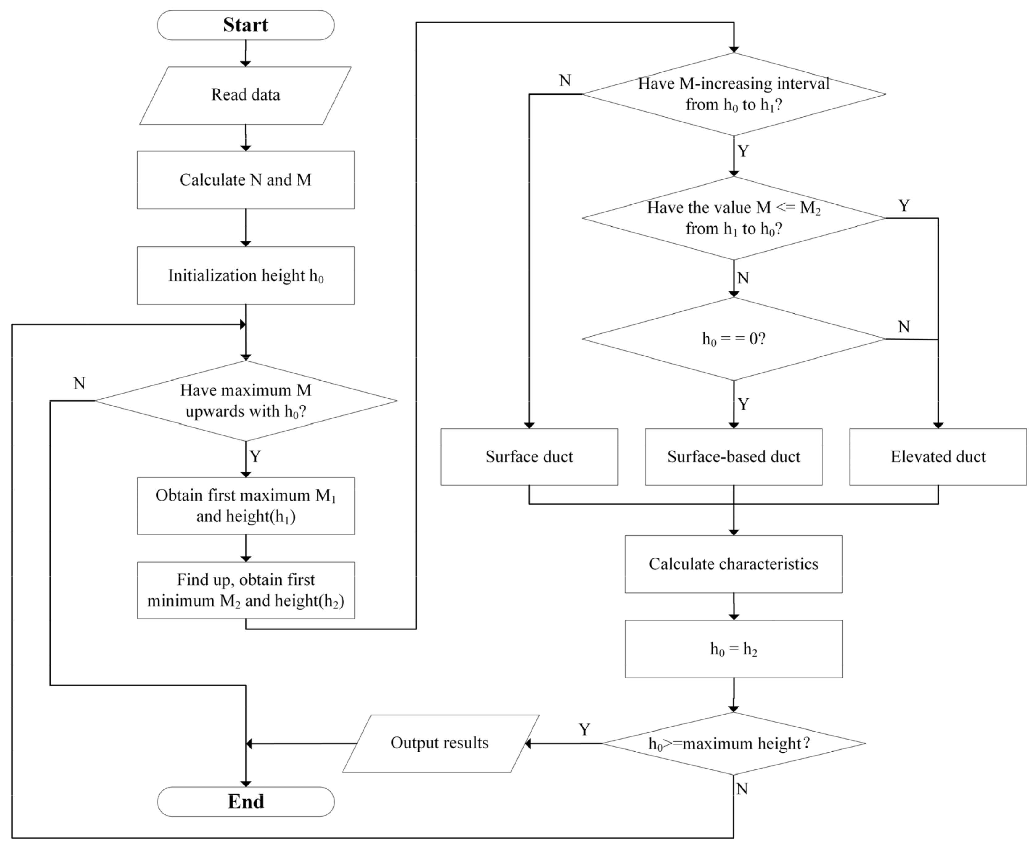
- The temperature, humidity, and other related variables were read from the model, and the modified atmospheric refractivity was calculated according to Formulas (1), (2), and (3). The height h0 = 0 was initialized, and whether a duct occurred starting from the lowest layer was checked;
- Starting from height h0, the first occurrence of a maximum peak of the modified refractivity was searched upwards, and the current height h1 (shown in blue in Figure 1) and the current modified refractivity M1 were then recorded. If there is no h1, it is determined that there is no duct, and the diagnosis is completed;
- If h1 exists, the search is continued upwards to determine the first minimum value of the modified refractivity. Next, the current height h2 and modified refractivity M2 were recorded;
- If there is no increased modified refractivity within the height of h0~h1, then the current duct is determined as a surface duct. At that time, the bottom height of the duct is 0 m. The top height of the duct is h2. The duct strength is M1–M2. The duct thickness is h2–h0;
- If there is an increased modified refractivity below the height of h1, the first point where the modified refractivity is less than M2 starting from h1 downwards is searched, and the height h3 at that point is recorded;
- If no points of less than M2 are found, and h0 is still the initial height of 0 m, the current duct is then identified as a surface-based duct. At that time, the bottom height of the duct is 0 m. The top height of the duct is h2. The duct strength is M1–M2. The duct thickness is h2–h0;
- If a point of less than M2 is found, the height h3 is recorded there, and it is determined that the current duct is an elevated duct. The bottom height of the duct is h3. The top height of the duct is h2. The duct strength is M1–M2, and the duct thickness is h2–h3;
- After the diagnosis process of the duct in this layer is completed, the initial height h0 is replaced with the height h2. Step b is now repeated, and the search is continued upwards to diagnose ducts in the next layer until the maximum height is reached.
2.3. Observation Data for Evaluation
3. Experimental Design
4. Results
4.1. Evaluation of the Mean Bias at All Radiosonde Stations
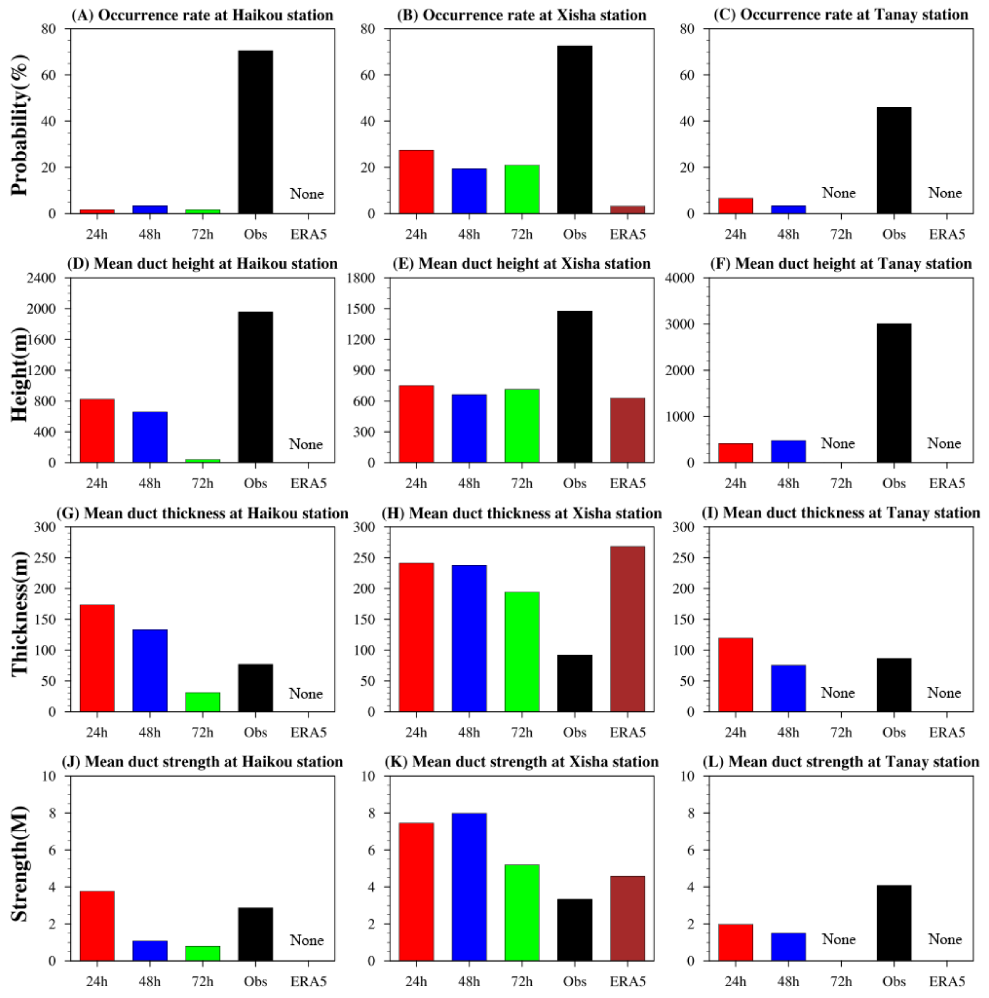
4.2. Evaluation of the Forecasted Duct Characteristics at Typical Stations
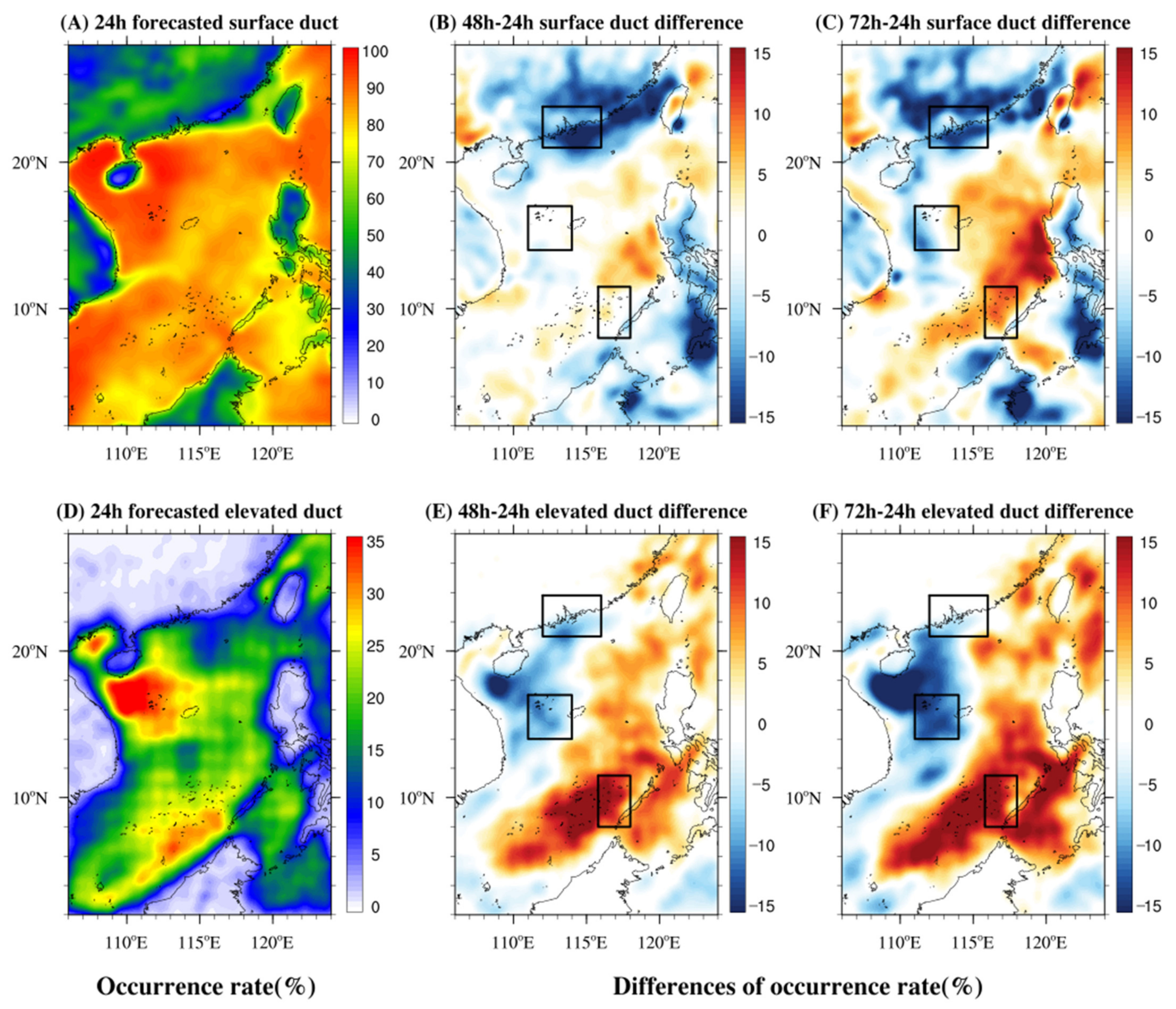
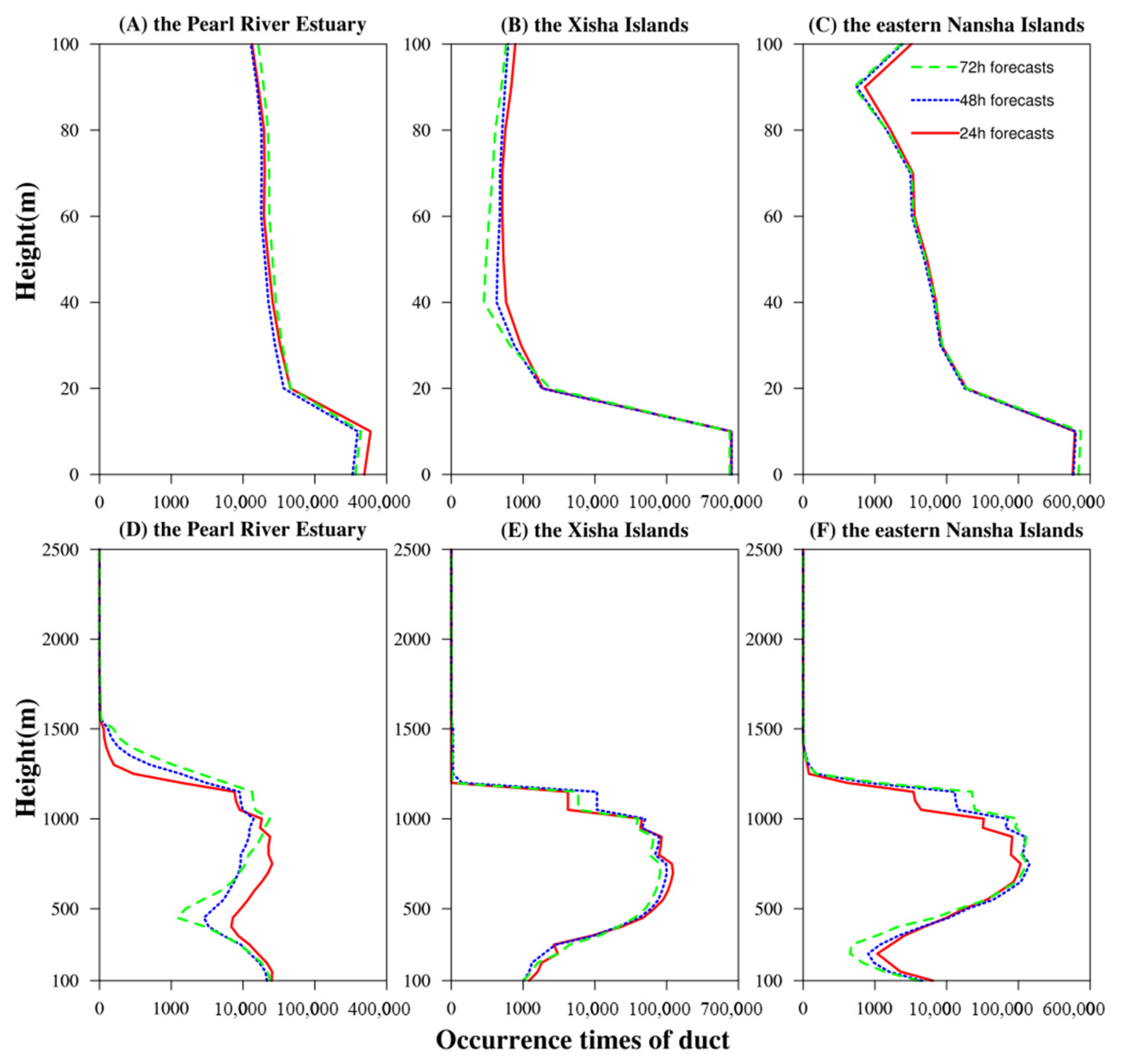
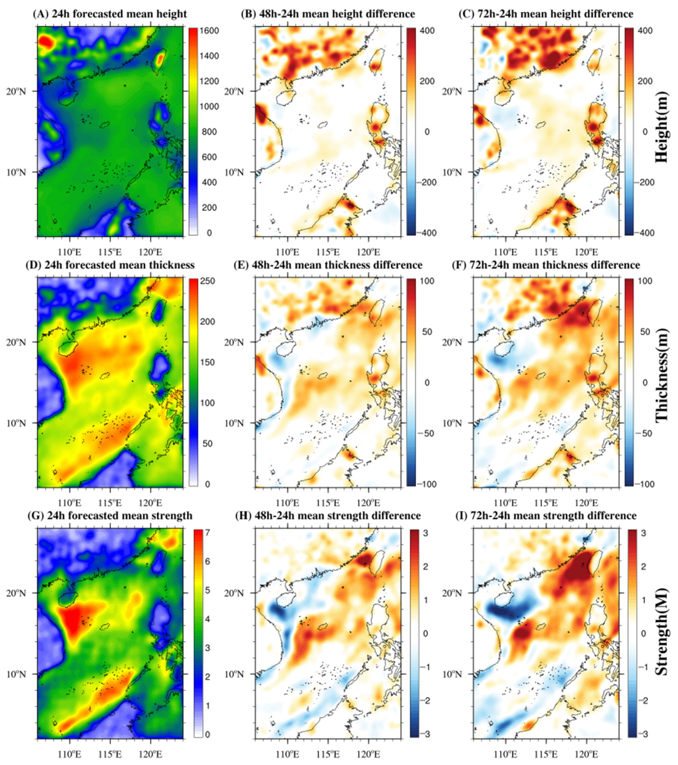
4.3. Spatial Distributions of the Forecasted Duct Characteristics over the Domain
5. Discussion
- In terms of model improvements, the physical parameterization schemes used in this study were obtained from sensitivity tests conducted in the previous studies for the China Seas. When applied in the South China Sea, the error of this scheme configuration may not be minimized. Therefore, a local optimization test specific to the South China Sea is needed to develop a scheme configuration with more minor errors. In addition, the assimilation process was not included in the forecasting simulation at this time. In the next step, the WRF data assimilation module will assimilate observation and satellite data to improve the duct forecasting accuracy further;
- In the simulation process, the model resolution also plays a crucial role in simulation accuracy. Previous studies have shown that high-resolution numerical models are capable of simulating finer-scale processes for structures or phenomena generated within a few hours, even without assimilation [37]. In this study, the horizontal resolution of the model was set to 12 km without using grid nesting to enhance the resolution. Such a resolution setting was sufficient for simulating a homogeneous marine environment but fell short in describing finer-scale processes such as coastal sea-land breezes. To validate this point, an additional nested forecasting test was conducted. The test ran from 00:00 UTC on 15 August 2021 to 00:00 UTC on 20 August 2021. The external grid remained at a 12 km resolution, while the internal grid had a resolution of 4 km. By comparing the mean bias of the modified atmospheric refractivity between the nested and original simulations, it was found that the higher-resolution nested simulation resulted in reduced errors by 12.2% and 3.2% at the Haikou and Tanay stations in coastal areas. However, for the Xisha Island station, which is closer to the marine environment, the nested test only reduced the error by 1.3%. This variation among stations suggested that marine weather forecasting was not highly sensitive to changes in model resolution, but coastal areas affected by finer-scale processes such as sea-land breezes were more sensitive to resolution changes. To enhance credibility, the analysis was further conducted at two island stations (Bach Longvi and Ranai) and two coastal stations (Kowloon and Kota Kinabalu) (see Figure 3 for station locations). The results demonstrated that at a resolution of 4 km, the modified atmospheric refractivity bias at the two island stations changed by only 1.1% and −2.1% compared to the original test at 12 km resolution, while the two coastal stations changed by 10.4% and −6.9%. It is important to note that this study primarily focuses on the South China Sea region, and a resolution of 12 km is sufficient for the analysis. However, future research will involve conducting more high-resolution simulations to analyze the effects of small-scale processes in coastal areas on the modified atmospheric refractivity and atmospheric ducting processes.
- In addition to horizontal resolution, the vertical resolution of the model also plays a significant role in the atmospheric ducting diagnosis process. To investigate the influence of model layering on duct diagnosis, three additional simulations were conducted with different vertical layering. One test reduced the model layers from 45 layers in the original test to 37 layers, and another test further reduced the vertical layers to 29 layers, which corresponds to the layers below 50 hPa in ERA5 data. The last one increased the layers to 53 layers. In the test with 37 layers, the eta values of the lowest 10 vertical levels in WRF are 1, 0.999, 0.998, 0.997, 0.995, 0.994, 0.993, 0.992, 0.990, and 0.987. In the test with 29 layers, the eta values of the lowest 10 vertical levels in WRF are 1, 0.998, 0.996, 0.993, 0.990, 0.974, 0.946, 0.905, 0.880, and 0.835. In the test with 53 layers, the eta values of the lowest 10 vertical levels in WRF are 1, 0.9998, 0.9995, 0.9992, 0.9985, 0.9981, 0.9979, 0.9975, 0.997, and 0.9965. The three tests ran from 00:00 UTC on 15 August 2021 to 00:00 UTC on 21 August 2021 for a total of 6 days. The numbers of ducts diagnosed from the tests and the original test are shown in Table 4. The results indicated that the number of ducts obtained from the numerical model was indeed related to the vertical layering of the model. The test with 29 layers diagnosed the lowest number of ducting cases, similar to the ERA5 data. The test with 37 layers diagnosed more ducting cases, while the test with 53 layers did not show significant differences from the original test. This suggested that a smaller number of vertical layers was not conducive to ducting diagnosis, and as the number of model layers increased, the vertical layering configuration was no longer a barrier to ducting diagnosis. In addition to the impact of changes to vertical layer density, it is worth noting that there may be some additional non-negligible impact from changes to the vertical location of those layers. It is still an outstanding unknown if more added layers are concentrated in the lowest few kilometers of the atmospheric column, and more detailed investigations should be made in the future.
- In terms of experimental design, the forecasting test only lasted for one month, which was too short to determine the long-term application effects of this duct prediction model. During the forecasting period, there were a few intense cyclones in the South China Sea. Therefore, the changes in ducts’ characteristics under extreme weather conditions were not discussed. In the future, it is necessary to conduct longer-term evaluations covering various types of weather to enhance the representativeness of the forecasting results;
- The observation data for evaluations in this study also need improvements in representativeness. Due to the inability of ERA5 reanalysis data to serve as an evaluation reference, this study only selected the sounding data from three stations to verify the ducts’ characteristics. The selection way of stations still had some randomness. Due to the scarcity of publicly available data, it is difficult for us to collect atmospheric-sounding data over the ocean. Therefore, this study could only be verified using publicly available sounding data from coastal areas or islands. Radiosonde stations located on several islands are less influenced by the interaction between sea and land processes, and their data are believed to be the closest to the marine environment. It was a pity that the sounding data were only available at two specific moments per day, and even so, there were some missing values in the sounding data. Therefore, more and denser marine observation data need to be collected in the future for more detailed evaluations;
- Due to space limitations, this study only considered the overall characteristics of surface and elevated ducts. It did not provide a more detailed classification and evaluation for each duct type, nor did it involve an analysis of the formation mechanism of ducts. The authors will conduct more in-depth research in the future.
6. Conclusions
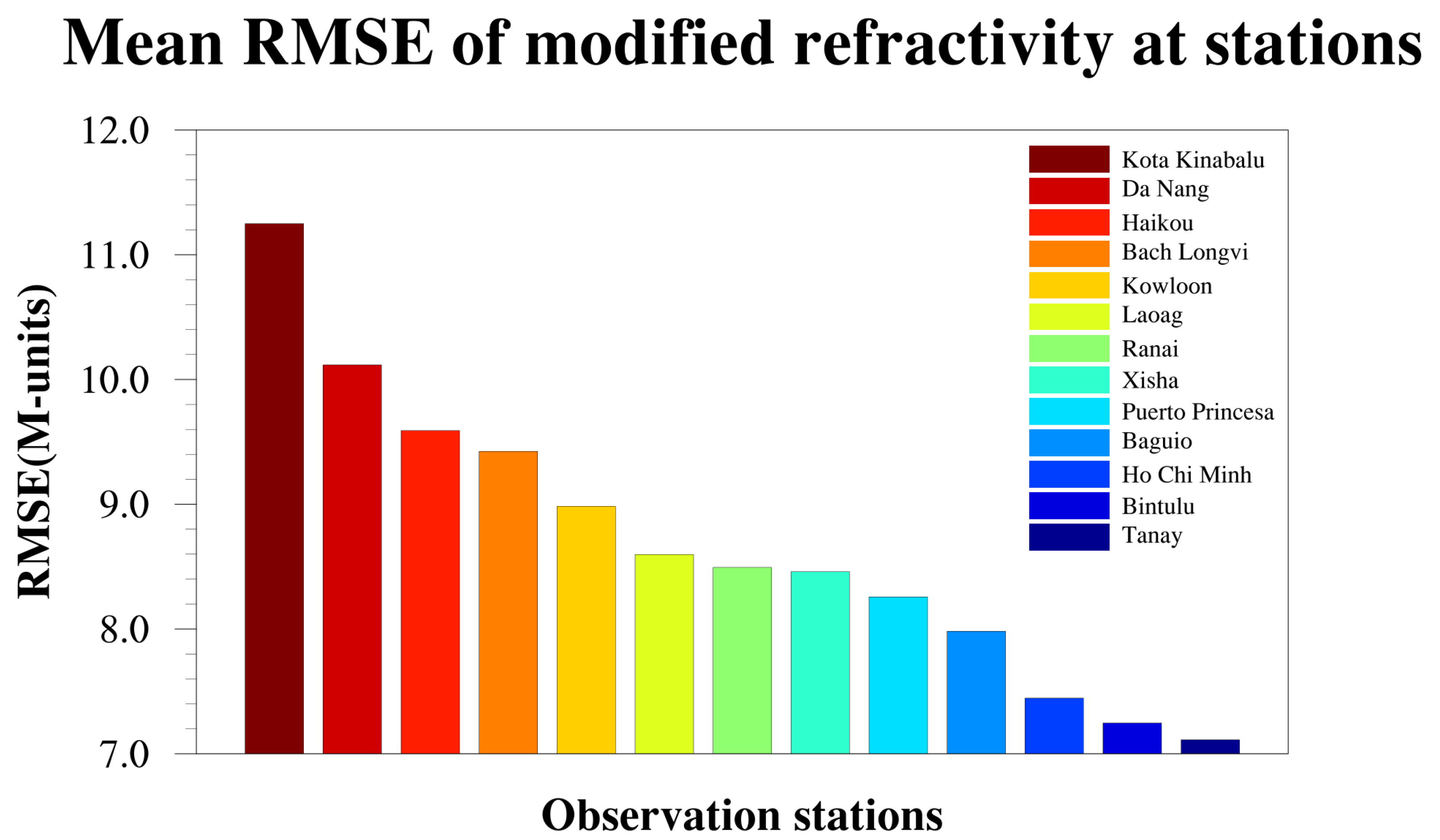
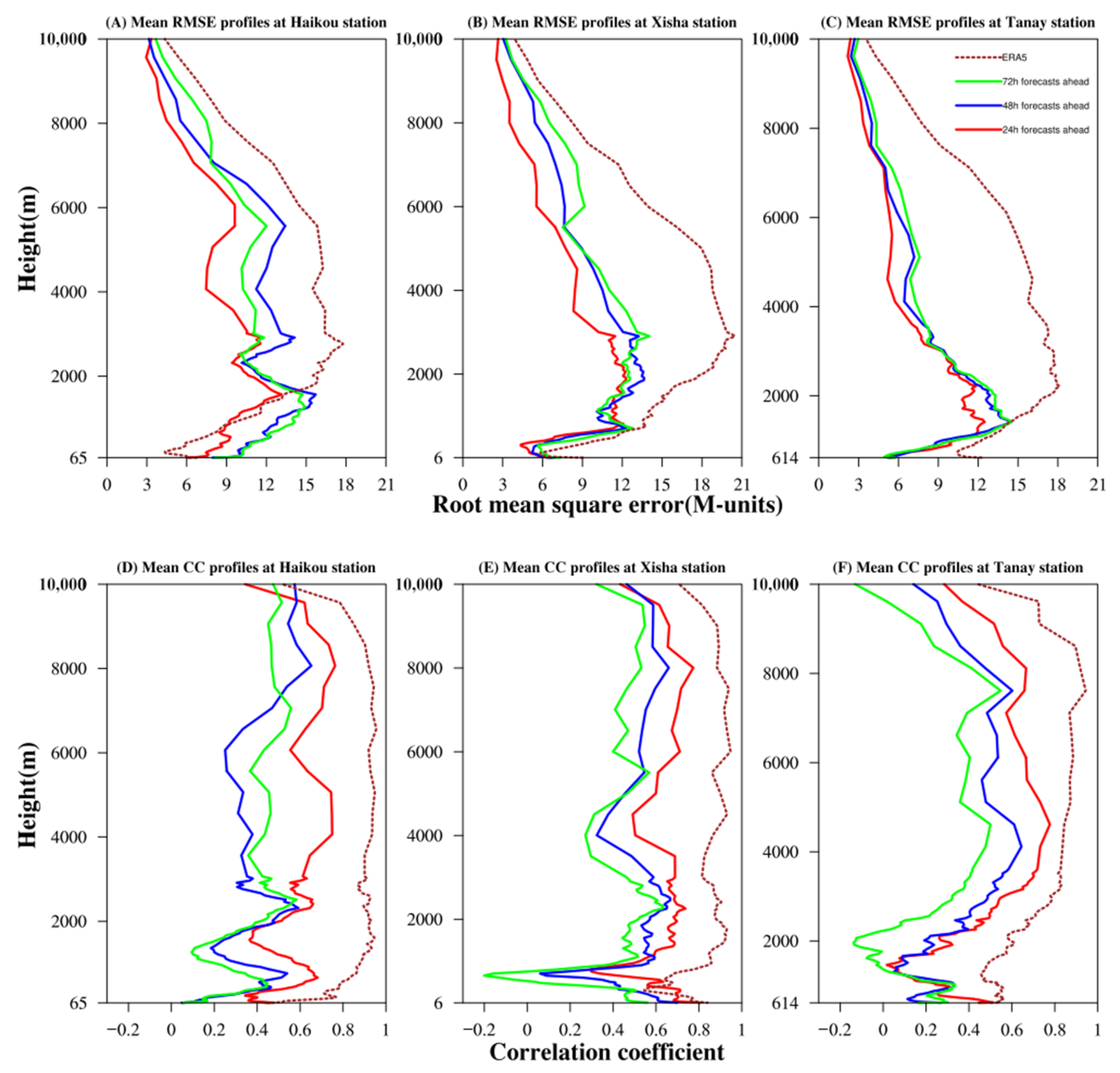
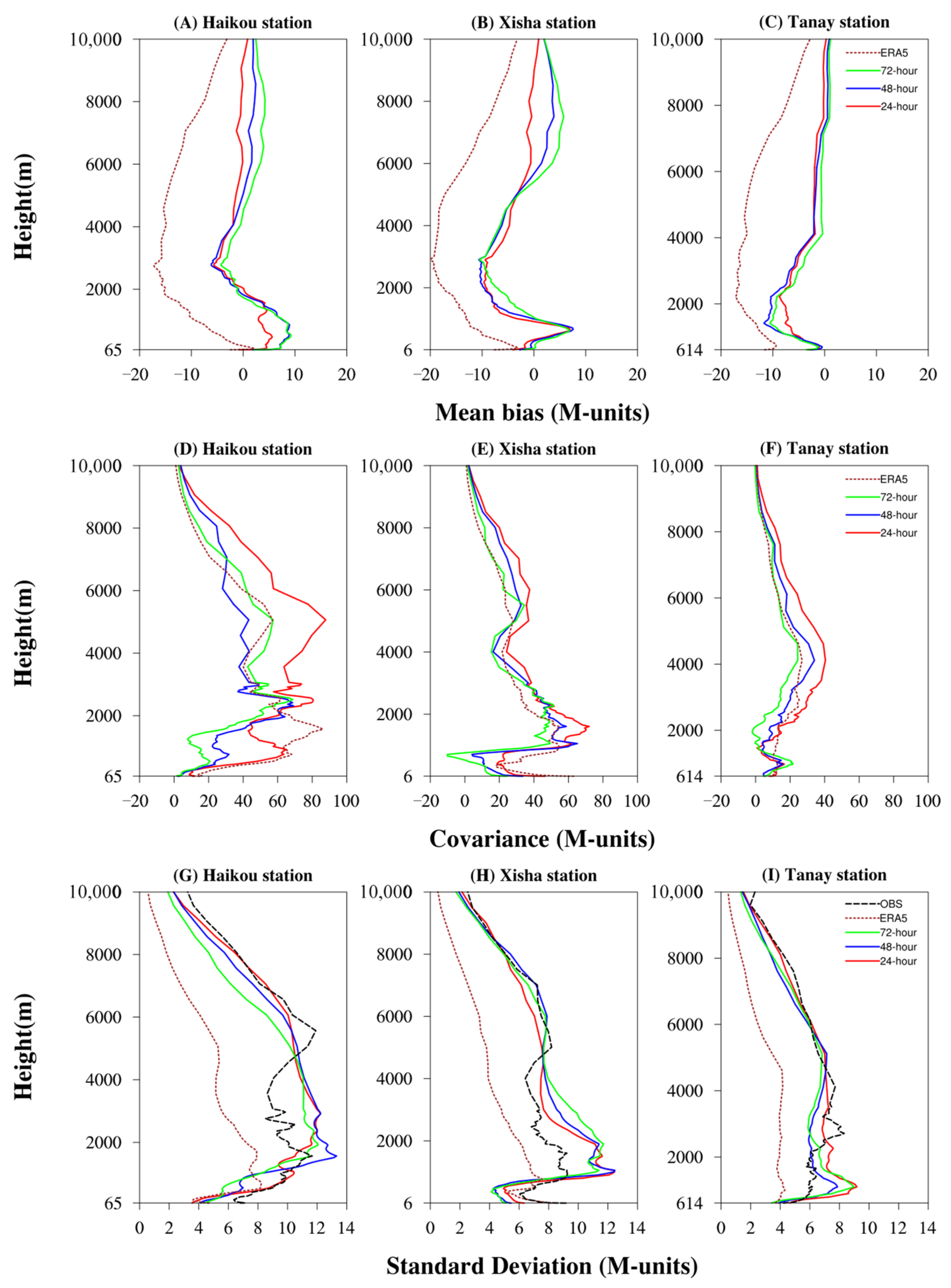
- During the simulation period in August 2021, the RMSEs of the predicted modified atmospheric refractivity were maintained between 7 M and 11.5 M at the 13 radiosonde stations around the South China Sea, with a high accuracy. The sounding data from three radiosonde stations with different error levels were selected for further evaluation. The results demonstrated that the predicted modified atmospheric refractivity could maintain a high accuracy in the forecasting time of 72 h, with minor changes in error. Compared with the observations, the maximum error of the predicted modified atmospheric refractivity appeared near the height of 2000 m, and the error gradually decreased with the increase in height. At the three stations, the RMSEs of the predicted modified atmospheric refractivity were generally lower than those of the ERA5 reanalysis data. However, the CCs of the forecasts with observations were slightly lower than the ERA5 data;
- The atmospheric duct characteristic parameters evaluations demonstrated that the duct forecasts 24 h ahead had the highest accuracy compared to the other two groups of tests. In the locations of Haikou, Xisha, and Tanay radiosonde stations, the predicted occurrence rates were generally lower than the diagnostic results from observations. The mean duct height, thickness, and strength were generally low, thin, and weak. This was because the predicted hourly modified refractivity gradient at each layer was smoother than the instantaneous observations with more randomness. The prediction accuracy was equivalent to the levels of duct forecasts using MetUM and other models in previous studies. The duct forecasting model established in this study, based on the ocean–atmosphere coupling model COAWST, was more suitable for marine duct forecasting. The forecasting accuracy at island radiosonde stations closer to the marine environment was higher than that in coastal areas. In addition, the prediction accuracy of surface ducts was generally higher than that of elevated ducts. This study also used the ERA5 reanalysis data for diagnosing ducts to enhance the reliability of the results. However, unfortunately, the ERA5 data could hardly be diagnosed with ducts and could not provide references for duct evaluation. This is due to the limited vertical resolution of ERA5 data below 2000 m, where atmospheric duct activity was more frequent. Subsequent sensitivity tests on vertical layers indicated that the diagnosed number of ducts increased with an increase in the number of vertical layers. Despite some uncertainties in these tests, the diagnosed duct number was proved not to continue to grow rapidly as the vertical layer number further increased. After surpassing 50 model layers, the growth of diagnosed duct numbers slowed down, and the number of vertical layers was not always the primary limiting factor for duct diagnosis;
- The spatial distributions of predicted surface and elevated ducts indicated that the duct occurrence rates at sea were significantly higher than on land. The occurrence rates of surface ducts were higher than those of elevated ducts in the same area. Throughout August, the occurrence rates of surface ducts accounted for about 85.5% of all duct events. The subsequent statistics over typical areas demonstrated that compared to the 24 h forecasts, fewer ducts occurred in the Pearl River Estuary and the Xisha Islands, with more ducts in the eastern Nansha Islands for the 48 h and 72 h forecasts. The most apparent differences in duct occurrence occurred at heights below 20 m and 500~1000 m. Furthermore, even after deducting terrain height, surface ducts occurring on lands were still higher, thicker, and stronger than at sea. The situation was reversed for elevated ducts, where the duct height, thickness, and strength at sea were generally higher than those on land. From the differences among the three groups of tests with different forecasting times, the differences in the duct height, thickness, and strength were consistent. Compared to the 24 h forecasts, the characteristics of surface ducts from the 48 h and 72 h forecasts were enhanced in the coastal areas of the northern South China Sea. The characteristics changes in elevated ducts were complicated. The duct parameters were enhanced in the northern and central regions of the South China Sea and weakened in the southern and western regions.
Author Contributions
Funding
Institutional Review Board Statement
Informed Consent Statement
Data Availability Statement
Conflicts of Interest
References
- Dinc, E.; Akan, O.B. Beyond-line-of-sight communications with ducting layer. IEEE Commun. Mag. 2014, 52, 37–43. [Google Scholar] [CrossRef]
- Yao, Z.; Zhao, B.; Li, W.; Zhu, Y.; Du, J.; Dai, F. Analysis on characteristics of atmospheric duct and its effects on the propagation of electromagnetic wave. J. Meteorol. Res. Prc. 2001, 15, 233–248. [Google Scholar]
- Hitney, H.V.; Richter, J.H.; Pappert, R.A.; Anderson, K.D.; Baumgartner, G.B. Tropospheric radio propagation assessment. Proc. IEEE 1985, 73, 265–283. [Google Scholar] [CrossRef]
- Babin, S.M.; Young, G.S.; Carton, J.A. A new model of the oceanic evaporation duct. J. Appl. Meteorol. Clim. 1997, 36, 193–204. [Google Scholar] [CrossRef]
- Bean, B.R.; Dutton, E.J. Radio Meteorology; Government Printing Office: Washington, DC, USA, 1966. [Google Scholar]
- Sirkova, I. Duct occurrence and characteristics for Bulgarian Black sea shore derived from ECMWF data. J. Atmos Sol. Terr. Phy. 2015, 135, 107–117. [Google Scholar] [CrossRef]
- Burk, S.D.; Thompson, W.T. Mesoscale modeling of summertime refractive conditions in the Southern California Bight. J. Appl. Meteorol. Clim. 1997, 36, 22–31. [Google Scholar] [CrossRef]
- Zhu, M.; Atkinson, B.W. Simulated climatology of atmospheric ducts over the Persian Gulf. Bound.-Lay. Meteorol. 2005, 115, 433–452. [Google Scholar] [CrossRef]
- Mentes, Ş.; Kaymaz, Z. Investigation of surface duct conditions over Istanbul, Turkey. J. Appl. Meteorol. Clim. 2007, 46, 318–337. [Google Scholar] [CrossRef]
- Xu, L.; Yardim, C.; Haack, T. Evaluation of COAMPS boundary layer refractivity forecast accuracy for 2–40 GHz electromagnetic wave propagation. Radio Sci. 2022, 57, 1–13. [Google Scholar] [CrossRef]
- Atkinson, B.W.; Li, J.G.; Plant, R.S. Numerical modeling of the propagation environment in the atmospheric boundary layer over the Persian Gulf. J. Appl. Meteorol. Clim. 2001, 40, 586–603. [Google Scholar] [CrossRef]
- Haack, T.; Wang, C.; Garrett, S.; Glazer, A.; Mailhot, J.; Marshall, R. Mesoscale modeling of boundary layer refractivity and atmospheric ducting. J. Appl. Meteorol. Clim. 2010, 49, 2437–2457. [Google Scholar] [CrossRef]
- Chai, X.; Li, J.; Zhao, J.; Wang, W.; Zhao, X. LGB-PHY: An evaporation duct height prediction model based on physically constrained lightGBM algorithm. Remote Sens. 2022, 14, 3448. [Google Scholar] [CrossRef]
- Lin, I.I.; Wu, C.C.; Emanuel, K.A.; Lee, I.H.; Wu, C.R.; Pun, I.F. The interaction of Supertyphoon Maemi (2003) with a warm ocean eddy. Mon. Weather Rev. 2005, 133, 2635–2649. [Google Scholar] [CrossRef]
- Liu, N.; Ling, T.; Wang, H.; Zhang, Y.; Gao, Z.; Wang, Y. Numerical simulation of Typhoon Muifa (2011) using a Coupled Ocean-Atmosphere-Wave-Sediment Transport (COAWST) modeling system. J. Ocean Univ. China 2015, 14, 199–209. [Google Scholar] [CrossRef]
- Zhu, J.; Zou, H.; Kong, L.; Zhou, L.; Li, P.; Cheng, W.; Bian, S. Surface atmospheric duct over Svalbard, Arctic, related to atmospheric and ocean conditions in winter. Arct. Antarct. Alp. Res. 2022, 54, 264–273. [Google Scholar] [CrossRef]
- Zou, J.; Zhan, C.; Song, H.; Hu, T.; Qiu, Z.; Wang, B.; Li, Z. Development and evaluation of a hydrometeorological forecasting system using the Coupled Ocean-Atmosphere-Wave-Sediment Transport (COAWST) Model. Adv. Meteorol. 2021, 2021, 1–17. [Google Scholar] [CrossRef]
- Wang, Q.; Alappattu, D.P.; Billingsley, S.; Blomquist, B.; Burkholder, R.J.; Christman, A.J.; Creegan, E.D.; de Paolo, T.; Eleuterio, D.P.; Fernando, H.J.S.; et al. CASPER: Coupled air–sea processes and electromagnetic ducting research. Bull. Am. Meteorol. Soc. 2018, 99, 1449–1471. [Google Scholar] [CrossRef]
- Warner, J.C.; Armstrong, B.; He, R.; Zambon, J.B. Development of a coupled ocean–atmosphere–wave–sediment transport (COAWST) modeling system. Ocean Model. 2010, 35, 230–244. [Google Scholar] [CrossRef]
- Jiao, D.; Xu, N.; Yang, F.; Xu, K. Evaluation of spatial-temporal variation performance of ERA5 precipitation data in China. Sci. Rep. 2021, 11, 17956. [Google Scholar] [CrossRef] [PubMed]
- Zou, J.; Lu, N.; Jiang, H.; Qin, J.; Yao, L.; Xin, Y.; Su, F. Performance of air temperature from ERA5-Land reanalysis in coastal urban agglomeration of Southeast China. Sci. Total Environ. 2022, 828, 154459. [Google Scholar] [CrossRef] [PubMed]
- Hong, S.Y.; Noh, Y.; Dudhia, J. A new vertical diffusion package with an explicit treatment of entrainment processes. Mon. Weather Rev. 2006, 134, 2318–2341. [Google Scholar] [CrossRef]
- Mlawer, E.J.; Taubman, S.J.; Brown, P.D.; Iacono, M.J.; Clough, S.A. Radiative transfer for inhomogeneous atmospheres: RRTM, a validated correlate-k model for the longwave. J. Geophys Res. Atmos. 1997, 102, 16663–16682. [Google Scholar] [CrossRef]
- Dudhia, J. Numerical study of convection observed during the winter monsoon experiment using a mesoscale two-dimensional model. J. Atmos. Sci. 1989, 46, 3077–3107. [Google Scholar] [CrossRef]
- Fairall, C.W.; Bradley, E.F.; Hare, J.E.; Grachev, A.A.; Edson, J.B. Bulk parameterization of air-sea fluxes: Updates and verification for the COARE algorithm. J. Climate 2003, 16, 571–591. [Google Scholar] [CrossRef]
- Tewari, M.; Chen, F.; Wang, W.; Dudhia, J.; LeMone, M.A.; Mitchell, K.; Ek, M.; Gayno, G.; Wegiel, J.W.; Cuenca, R. Implementation and verification of the unified NOAH land surface model in the WRF model. In Proceedings of the 20th Conference on Weather Analysis and Forecasting/16th Conference on Numerical Weather Prediction, Seattle, WA, USA, 14 January 2004. [Google Scholar]
- Bae, S.Y.; Hong, S.; Tao, W. Development of a Single-Moment Cloud Microphysics Scheme with Prognostic Hail for the Weather Research and Forecasting (WRF) Model. Asia-Pac. J. Atmos. Sci. 2018, 55, 233–245. [Google Scholar] [CrossRef]
- Grell, G.A.; Freitas, S.R. A scale and aerosol aware stochastic convective parameterization for weather and air quality modeling. Atmos. Chem. Phys. 2014, 14, 5233–5250. [Google Scholar] [CrossRef]
- Mellor, G.; Yamada, T. Development of a turbulence closure model for geophysical fluid problems. Rev. Geophys. 1982, 20, 851–875. [Google Scholar] [CrossRef]
- Wang, X.; Chao, Y.; Dong, C.; Farrara, J.; Li, Z.; McWilliams, J.C.; Paduan, J.D.; Rosenfeld, L.K. Modeling tides in Monterey Bay, California. Deep. Sea Res. Pt. II 2009, 56, 219–231. [Google Scholar] [CrossRef]
- Chai, T.; Draxler, R.R. Root mean square error (RMSE) or mean absolute error (MAE)?—Arguments against avoiding RMSE in the literature. Geosci. Model. Dev. 2014, 7, 1247–1250. [Google Scholar] [CrossRef]
- Adler, J.; Parmryd, I. Quantifying colocalization by correlation: The Pearson correlation coefficient is superior to the Mander’s overlap coefficient. Cytom. Part A 2010, 77, 733–742. [Google Scholar] [CrossRef] [PubMed]
- Lee, D.K.; In, J.; Lee, S. Standard deviation and standard error of the mean. Korean J. Anesthesiol. 2015, 68, 220–223. [Google Scholar] [CrossRef] [PubMed]
- Roebber, P.J. Visualizing multiple measures of forecast quality. Weather Forecast. 2009, 24, 601–608. [Google Scholar] [CrossRef]
- Shi, Y.; Wang, S.; Yang, F.; Yang, K. Statistical Analysis of Hybrid Atmospheric Ducts over the Northern South China Sea and Their Influence on Over-the-Horizon Electromagnetic Wave Propagation. J. Mar. Sci. Eng. 2023, 11, 669. [Google Scholar] [CrossRef]
- Zhou, Y.; Liu, Y.; Qiao, J.; Li, J.; Zhou, C. Statistical Analysis of the Spatiotemporal Distribution of Lower Atmospheric Ducts over the Seas Adjacent to China, Based on the ECMWF Reanalysis Dataset. Remote. Sens. 2022, 14, 4864. [Google Scholar] [CrossRef]
- Skamarock, W.C. Evaluating mesoscale NWP models using kinetic energy spectra. Mon. Weather Rev. 2004, 132, 3019–3032. [Google Scholar] [CrossRef]


| WRF | ROMS | SWAN | |
|---|---|---|---|
| Number of grid points | 180 × 260 | 170 × 240 | 170 × 240 |
| Horizontal resolution | 12 km × 12 km | 12 km × 12 km | 12 km × 12 km |
| Vertical levels | 45 | 16 | 1 |
| Driving data | GFS | RTOFS | GFS_wave |
| Time step | 30 s | 30 s | 600 s |
| Surface Duct | Elevated Duct | ||||||
|---|---|---|---|---|---|---|---|
| Haikou | Xisha | Tanay | Haikou | Xisha | Tanay | ||
| Hit rate | 24 h | 26.32% | 100% | 20% | 2.33% | 31.11% | 7.14% |
| 48 h | 18.42% | 96.67% | 10% | 4.65% | 24.44% | 3.57% | |
| 72 h | 18.42% | 93.33% | 0% | 2.33% | 22.22% | 0% | |
| ERA5 | 0% | 0% | 0% | 0% | 4.44% | 0% | |
| FAR | 24 h | 44.44% | 46.43% | 66.67% | 0% | 17.65% | 50% |
| 48 h | 46.15% | 50.85% | 66.67% | 0% | 8.33% | 50% | |
| 72 h | 58.82% | 52.54% | 100% | 0% | 23.08% | 0% | |
| ERA5 | 0% | 0% | 0% | 0% | 0% | 0% | |
| CSI | 24 h | 0.22 | 0.54 | 0.14 | 0.02 | 0.29 | 0.07 |
| 48 h | 0.16 | 0.48 | 0.08 | 0.05 | 0.24 | 0.03 | |
| 72 h | 0.15 | 0.46 | 0 | 0.02 | 0.21 | 0 | |
| ERA5 | 0 | 0 | 0 | 0 | 0.04 | 0 | |
| Surface Variable | Surface Duct | Elevated Duct | ||||
|---|---|---|---|---|---|---|
| 24 h Forecasts | 48 h Forecasts | 72 h Forecasts | 24 h Forecasts | 48 h Forecasts | 72 h Forecasts | |
| SST | 0.86 | 0.84 | 0.84 | 0.68 | 0.63 | 0.62 |
| T2m | 0.56 | 0.53 | 0.52 | 0.41 | 0.33 | 0.30 |
| RH2m | −0.15 | −0.16 | −0.14 | −0.04 | 0.04 | 0.07 |
| SLP | 0.58 | 0.55 | 0.55 | 0.52 | 0.48 | 0.48 |
| Wind speed | 0.41 | 0.44 | 0.43 | 0.47 | 0.36 | 0.27 |
| Surface Duct | Elevated Duct | ||||||
|---|---|---|---|---|---|---|---|
| Haikou | Xisha | Tanay | Haikou | Xisha | Tanay | ||
| Test with 53 layers | 78 | 149 | 14 | 6 | 44 | 3 | |
| Original test (45 layers) | 76 | 144 | 12 | 2 | 40 | 2 | |
| Test with 37 layers | 32 | 93 | 0 | 7 | 0 | 0 | |
| Test with 29 layers | 6 | 0 | 0 | 2 | 0 | 0 | |
| ERA5 (29 layers) | 0 | 0 | 0 | 0 | 2 | 0 | |
Disclaimer/Publisher’s Note: The statements, opinions and data contained in all publications are solely those of the individual author(s) and contributor(s) and not of MDPI and/or the editor(s). MDPI and/or the editor(s) disclaim responsibility for any injury to people or property resulting from any ideas, methods, instructions or products referred to in the content. |
© 2024 by the authors. Licensee MDPI, Basel, Switzerland. This article is an open access article distributed under the terms and conditions of the Creative Commons Attribution (CC BY) license (https://creativecommons.org/licenses/by/4.0/).
Share and Cite
Liu, Q.; Zhao, X.; Zou, J.; Li, Y.; Qiu, Z.; Hu, T.; Wang, B.; Li, Z. Development of a Numerical Prediction Model for Marine Lower Atmospheric Ducts and Its Evaluation across the South China Sea. J. Mar. Sci. Eng. 2024, 12, 141. https://doi.org/10.3390/jmse12010141
Liu Q, Zhao X, Zou J, Li Y, Qiu Z, Hu T, Wang B, Li Z. Development of a Numerical Prediction Model for Marine Lower Atmospheric Ducts and Its Evaluation across the South China Sea. Journal of Marine Science and Engineering. 2024; 12(1):141. https://doi.org/10.3390/jmse12010141
Chicago/Turabian StyleLiu, Qian, Xiaofeng Zhao, Jing Zou, Yunzhou Li, Zhijin Qiu, Tong Hu, Bo Wang, and Zhiqian Li. 2024. "Development of a Numerical Prediction Model for Marine Lower Atmospheric Ducts and Its Evaluation across the South China Sea" Journal of Marine Science and Engineering 12, no. 1: 141. https://doi.org/10.3390/jmse12010141
APA StyleLiu, Q., Zhao, X., Zou, J., Li, Y., Qiu, Z., Hu, T., Wang, B., & Li, Z. (2024). Development of a Numerical Prediction Model for Marine Lower Atmospheric Ducts and Its Evaluation across the South China Sea. Journal of Marine Science and Engineering, 12(1), 141. https://doi.org/10.3390/jmse12010141