Short-Term Prediction of Ship Roll Motion in Waves Based on Convolutional Neural Network

Abstract

In this study, a short-term prediction method for ship roll motion in waves based on convolutional neural network (CNN) is presented. Firstly, based on the ship roll motion equation, the data for free roll attenuation motion in still water, roll motion in regular waves, and roll motion excited by irregular waves are simulated, respectively. Secondly, the simulation data is normalized and preprocessed, and then the time-sliding window technique is applied to construct the training and testing sample sets. Thirdly, the CNN model is trained by learning from the constructed training sample sets, and the well-trained CNN model is applied to predict the roll motion. To validate the CNN model’s prediction accuracy and effectiveness, a comparison between the forecasted results and the simulation data is conducted. Meanwhile, the predicted results are also compared with that of the long-short-term memory (LSTM) neural network. The research results demonstrate that CNN can effectively achieve accurate prediction of ship roll motion in waves, and its prediction accuracy is the same as that of the LSTM neural network.

1. Introduction

As a ship navigates in open waters, it becomes subject to a range of environmental elements, including winds, waves, and currents. Under certain conditions, a large roll motion will occur, which seriously threatens the navigation safety of the ship. In order to guarantee ship navigation safety at sea, precise anticipation of ships’ nonlinear roll movements is imperative. For this purpose, three kinds of method have been successively put forward [1]. The first kind of prediction method is based on ship hydrodynamics theory. The mathematical model of roll motion is established according to ship hydrodynamics, and the damping coefficients in the mathematical model are obtained by means of model tests or CFD simulations. Hashimoto et al. [2] and Kianejad et al. [3] forecasted the roll motion by the motion model with the obtained damping coefficients. In order to predict the ship roll motion, Kianejad et al. [4] used the CFD method to calculate the damping coefficients; Liu et al. [5] used CFD to predict the parametric roll characteristics; and Chen et al. [6] used the CFD method to establish a numerical model of ship motion coupled with fluid motion.

The second kind of prediction method is based on the time series model. By regression analysis of historical time series data of ship roll motion, time series models of ship roll motion in waves was used to predict ship roll motion. Jiang et al. [7] and Selvaraj et al. [8] used the auto-regressive model (AR model) and auto-regressive integrated moving average model (ARIMA model) to predict ship roll motion, respectively. The third kind of prediction method is the data-driven prediction method based on machine learning techniques. By means of machine learning algorithms, the inherent mechanism of ship roll motion is learned from the collected mass of ship roll motion data, and the nonparametric black-box model of ship roll motion is constructed. For example, Yin et al. [9] and Huang et al. [10] applied the variable structure RBF neural network and wavelet neural network to predict ship roll motion, respectively. Chen et al. [11] applied the support vector machine to identify the mathematical model of ship roll motion in shallow water. Suhermi et al. [12] combined the deep forward neural network and ARIMA model to predict ship roll motion.

In recent years, deep neural networks have been applied to solve pattern recognition, function fitting, etc. Xue et al. [13] applied the convolutional neural network to pattern recognition. Belomestny et al. [14] applied deep neural networks to approximate the nonlinear function and its derivatives simultaneously. Rithani et al. [15] discussed the benefits and drawbacks of various deep neural networks for big data analysis. The most common deep neural networks include deep recurrent neural network (RNN) and convolutional neural network (CNN). In contrast to the traditional RNN, the long-short-term memory (LSTM) neural network, a derivative of RNN, reduces the risk of gradient explosion/disappearance during neural network training. Hochreiter et al. [16] achieved this by incorporating an architecture comprising input gate, forgetting gate, output gate, and state storage unit, which effectively regulates neuron states. In the field of ship motion attitude prediction, machine learning has a stronger ability to extract complex nonlinear features and map them to output, compared with mathematical models and statistical models. Therefore, it was applied to predict ship motion by some researchers. Huang et al. [10] established a ship roll motion prediction model, which fully utilizes the fitting ability of conventional neural networks. Zhang et al. [17], Zhang et al. [18] and Wei et al. [19] conducted prediction studies on ship roll motion by the LSTM neural network, respectively. Jiang et al. [20] applied the LSTM neural network to a non-parametric identification model and prediction of ship maneuvering motion. Wang et al. [21] proposed a ship roll angle prediction method based on bidirectional long short-term memory network and temporal pattern attention mechanism combined deep learning model to improve the accuracy of ship roll angle prediction. Sun et al. [22] combined LSTM and Gauss process regression technology to predict ship roll motion and pitch motion, respectively. However, there is relatively little research using convolutional neural network to predict ship roll motion in waves. Further validation is required to assess the effectiveness and robustness of ship roll motion prediction technology by using deep neural networks.

In this paper, CNN is used to predict ship roll motion in the short term. Firstly, CNN is used to predict the free roll decay motion in still water. Secondly, the roll motion in regular waves is predicted by CNN. Thirdly, the roll motion excited by six different irregular wave spectra are respectively simulated, and then the simulation data are learned by CNN. To demonstrate the prediction effect, the prediction results of CNN are compared with that of the LSTM neural network. Through this study, it can be found that the CNN model can predict complex nonlinear phenomena through reasonable training. In addition, the method is not limited by the physical model and has strong prediction performance.

2. Convolutional Neural Network

Convolutional neural network (CNN) is a kind of deep feed-forward neural network, including convolutional computation, and is used especially to process data, similarly to grid structures. By using the gradient descent method, CNN realizes layer-by-layer reverse adjustment of the weight parameters in the network. The prediction accuracy of CNN is improved by iterative training. At present, several deep learning models based on convolutional neural networks, such as AlexNet [23], VGG [24], GoogLeNet [25] and ResNet [26] have been proposed successively and have been widely used in image processing and pattern recognition.

Typically, three types of neuron layers, convolutional layer, pooling layer and fully connected layer, together make up the CNN structure. It extracts data features through multi-level nonlinear modules, connects adjacent nodes of the same level through convolution calculation, and carries out feature extraction step by step from low level to high level, so as to construct complex features with multiple levels of abstraction.

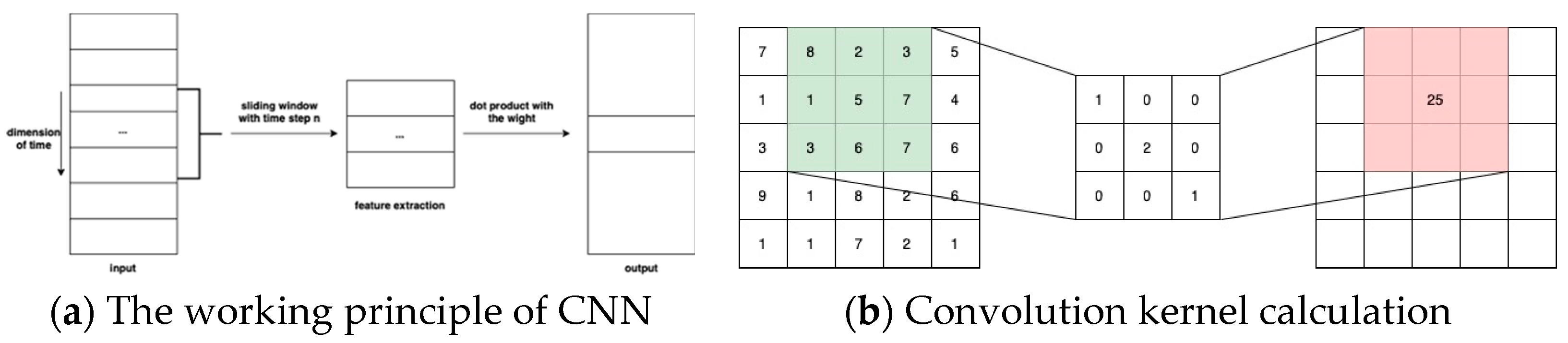
Figure 1a depicts the computational principle of CNN. The convolution kernel of CNN slides on the time series data. Since the data it processes each time is in a time window, instead of the data at a certain moment, CNN can extract the changing relationship of the sequence data reflected in the time dimension. Figure 1b simply shows the convolution operation principle of convolution kernel: the $5\times 5$ matrix on the left is the input original data, the $3\times 3$ matrix in the middle is the convolution kernel, and on the right is the output data. The convolution kernel is a sliding window that moves with a fixed step from left to right and from top to bottom on the original data. Each element in the convolution kernel has a fixed weight and bias. The operation rule adopted by the convolution calculation in CNN is that the original data is multiplied by the convolution kernel and then added, which is expressed as:

$$\{\begin{array}{l}{y}_n(i,j)={\displaystyle \sum _{k=1}^{k_{n-1}}{\displaystyle \sum _{m=1}^w{\displaystyle \sum _{z=1}^h\left[y_{n-1}^k(si+m,sj+z)W_n^k(m,z)\right]+b_n}}}\\ L_n\left(w\right)=\frac{L_{n-1}\left(w\right)+2p-w}{s}+1\\ L_n\left(h\right)=\frac{L_{n-1}(h)+2p-h}{s}+1\end{array}$$

(1)

where $y_n\left(i,j\right)$ is the element whose coordinate is $\left(i,j\right)$ in the output data of the n convolution layer; $y_{n-1}\left(i,j\right)$ is the element whose coordinate is $\left(i,j\right)$ in the input data of the n − 1 convolution layer; k is the number of channels; w is the width of the convolution kernel; h is the height of the convolution kernel; s is the convolution step; $b_n$ is the bias parameter of the n convolution layer; p is the number of fills; $L_n\left(w\right)$ is the width of $y_n\left(i,j\right)$; and $L_n\left(h\right)$ is the height of $y_n\left(i,j\right)$.

As mentioned above, the convolution kernel slides on the same layer of data and shares a set of convolution kernel parameters during data feature extraction at each position, meaning that the CNN model features sparse connections and parameter sharing. Compared with the fully connected neural network, the number of parameters of CNN is greatly reduced and the learning rate is accelerated. Moreover, the pooling layer of CNN divides the data into several regions and outputs the maximum or average value of the data in each sub-region. This approach trims the amount of data processing and retains the valuable information, and thus improves the processing efficiency and reduces overfitting. After several operations of the convolution layer and pooling layer, the output of CNN is obtained by the calculation of the fully connected layer.

When applied CNN to predict ship roll motion, the basic steps are as follows (see Figure 2).

Firstly, based on the obtained data sample set, the training sample set and the test sample set were constructed. In this article, the data sample set was obtained by numerical simulation according to ship roll motion equation. Then, the sample set was split into the training sample set and the test sample set according to a ratio of 0.7. The first 70% of the data was the training sample set, and the last 30% of the data was the testing sample set.

Secondly, a convolutional neural network predicted model was established. Therein, the input and output dimensions of the CNN, the hyper-parameters, number of convolutional layers, pooling method, learning rate and activation function, etc., were determined in advance.

Thirdly, use the training sample set to train the established CNN model and evaluate the training result by the learning loss, and determine whether adjustment of the CNN parameters was needed.

Finally, based on the trained model, the test sample set was predicted, and the predicted error was also calculated to evaluate the predicted accuracy.

3. Roll Motion Equation of Ships

According to ship hydrodynamics, the roll motion equation of a ship in waves can be described by a second-order nonlinear differential equation:

$$(I_{xx}+J_{xx})\ddot{\varphi }+D(\dot{\varphi })+R(\varphi )=F$$

(2)

where $\varphi$ is the angle of roll (rad); $I_{xx}$ is the roll moment of inertia $(\mathrm{k}\mathrm{g}·{\mathrm{m}}^2)$; $J_{xx}$ is the additional moment of inertia $(\mathrm{k}\mathrm{g}·{\mathrm{m}}^2)$; $D\left(\dot{\varphi }\right)$ is roll damping $(\mathrm{N}·\mathrm{m})$; $R\left(\varphi \right)$ is roll restoring moment $(\mathrm{N}·\mathrm{m})$; and F is the wave excitation moment $(\mathrm{N}·\mathrm{m})$.

For the purpose of achieving precise prediction of ship roll motion, the key is to accurately determine the damping of roll motion in waves. According to Ikeda’s theory [27], roll damping is mainly composed of friction damping, vortex damping, lift damping, wave damping and bilge keel damping. However, each part is coupled together, and it is difficult to determine each part separately in practice. To predict roll damping, it is usually expanded as a function of roll angular rate:

$$D(\dot{\varphi })=D_1\dot{\varphi }+D_2\left|\dot{\varphi }\right|\dot{\varphi }+D_3{\dot{\varphi }}^3+\cdots$$

(3)

where $D_i,i=1,2,3,\cdots$ are linear or nonlinear damping coefficients. In practical applications, the nonlinear roll damping of ships is commonly represented by combining linear components with quadratic or cubic terms:

$$D(\dot{\varphi })=D_1\dot{\varphi }+D_2\left|\dot{\varphi }\right|\dot{\varphi },or,D(\dot{\varphi })=D_1\dot{\varphi }+D_3{\dot{\varphi }}^3$$

(4)

The restoring moment of ship roll is expressed as an odd function of roll angle:

$$R(\varphi )=R_1\varphi +R_3{\varphi }^3+R_5{\varphi }^5+\cdots ={\displaystyle \sum R_{2i-1}{\varphi }^{2i-1}},i=1,2,3,\dots$$

(5)

where $R_{2i-1},i=1,2,3,\cdots$ are linear or nonlinear restoring moment coefficients:

By introducing Equations (3) and (5) into Equation (2), the rolling motion equation of a ship in waves can be written:

$$(I_{xx}+J_{xx})\ddot{\varphi }+D_1\dot{\varphi }+D_2\left|\dot{\varphi }\right|\dot{\varphi }+D_3{\dot{\varphi }}^3+\cdots +R_1\varphi +R_3{\varphi }^3+R_5{\varphi }^5+\cdots =F$$

(6)

Perform division on both sides of Equation (6) by $\left(I_{xx}+J_{xx}\right)$, and the ship roll motion equation can be normalized as:

$$\ddot{\varphi }+d_1\dot{\varphi }+d_2\left|\dot{\varphi }\right|\dot{\varphi }+d_3{\dot{\varphi }}^3+\cdots +r_1\varphi +r_3{\varphi }^3+r_5{\varphi }^5+\cdots =f$$

(7)

where $f=F/\left(I_{xx}+J_{xx}\right)$; $d_i=D_i/\left(I_{xx}+J_{xx}\right);\mathrm{a}\mathrm{n}\mathrm{d}{r}_i=R_i/\left(I_{xx}+J_{xx}\right)$.

When a ship performs free roll attenuation motion in still water, the wave excitation is zero. The equation describing the free roll decay motion can be formulated as:

$$\ddot{\varphi }+d_1\dot{\varphi }+d_2\left|\dot{\varphi }\right|\dot{\varphi }+d_3{\dot{\varphi }}^3+\cdots +r_1\varphi +r_3{\varphi }^3+r_5{\varphi }^5+\cdots =0$$

(8)

When a ship rolls in regular waves, the moment generated by wave excitation can be expressed as:

$$f=f_A\cos ({\omega }_{e}t+\beta )=f_1\cos {\omega }_{e}t+f_2\sin {\omega }_{e}t$$

(9)

where $f_A$ is the amplitude of wave excitation moment; ${\omega }_e$ is the wave encounter frequency of ship roll motion; and $\beta$ is the phase difference; $f_1=f_A\cos \beta$; $f_2=-f_A\sin \beta$.

By substituting Equation (9) into rolling motion Equation (7), the equation depicting the rolling motion of a ship in regular waves can be expressed as:

$$\ddot{\varphi }+d_1\dot{\varphi }+d_2\left|\dot{\varphi }\right|\dot{\varphi }+d_3{\dot{\varphi }}^3+\cdots +r_1\varphi +r_3{\varphi }^3+r_5{\varphi }^5+\cdots =f_1\cos {\omega }_{e}t+f_2\sin {\omega }_{e}t$$

(10)

As a ship navigates through irregular waves, the wave excitation moment and the roll motion are also irregular. According to the superposition principle, the irregular wave excitation can be interpreted as the cumulative effect of multiple regular wave excitations, characterized by different amplitudes, frequencies and random phases:

$$f={\displaystyle \sum _{i=1}^{\infty }{f}_{i,A}\cos \left({\omega }_{i}t+{\theta }_i\right)}$$

(11)

where ${\omega }_i$ is the frequency of each component; and ${\theta }_i$ is the phase of each component, uniformly distributed in the interval [0, 2π].

By substituting Equation (11) into Equation (7), the equation governing the roll motion of a ship under irregular waves can be formulated as:

$$\ddot{\varphi }+d_1\dot{\varphi }+d_2\left|\dot{\varphi }\right|\dot{\varphi }+d_3{\dot{\varphi }}^3+\cdots +r_1\varphi +r_3{\varphi }^3+r_5{\varphi }^5+\cdots ={\displaystyle \sum _{i=1}^{\infty }{f}_{i,A}\cos \left({\omega }_{i}t+{\theta }_i\right)}$$

(12)

4. Training Model Setting

In this paper, a new designed ship for marine aquaculture was selected to be analyzed. The full-scaled ship parameters are listed in

Table 1. Ship information.

Parameter	Value	Unit
Length between perpendiculars	250.00	m
Breadth	43.95	m
Depth	27.25	m
Block coefficient	0.85	-

. The scale ratio of the ship model used in this study is 1/42.

4.1. Data Preprocessing

For the purpose of validating the applicability and accuracy of the deep neural network model, it is necessary to prepare the data set for training deep neural networks in advance.

In order to obtain the data for ship free roll decay motion in still water, linear and quadratic damping was used. Meanwhile, the linear and cubic restoring moment and the used free roll decay motion equation were rewritten as

$$\ddot{\varphi }+d_1\dot{\varphi }+d_2\left|\dot{\varphi }\right|\dot{\varphi }+r_1\varphi +r_3{\varphi }^3=0$$

(13)

The nonlinear damping coefficient and restoring moment coefficient were determined by using ship hydrodynamics in advance. The damping and restoring moment coefficients were d₁ = 0.002576, d₂ = −0.004437, r₁ = 0.3950, r₃ = 0.6348. The initial angle was set to 0.262 rad and the time step size was h = 0.05 s, and the fourth-order Runge–Kutta method was used to solve the free roll decay motion equation. The obtained roll motion is shown in Figure 3.

To obtain the roll motion in regular waves, linear and quadratic damping was used, and the linear and cubic restoring moment was used. The wave amplitude was 0.118 m and wave frequency was 0.45 rad/s. The simulated rolling motion is shown in Figure 4.

In order to validate the prediction effect of CNN, the roll motion under six different irregular wave spectrum excitations was simulated, and the simulated roll responses were used to construct the sample set.

The white noise spectrum excitation consists of 70 cosine functions with an amplitude of 0.07 rad/s² at equal frequency intervals. The frequency range is selected from 2.0 to 5.0 rad/s, which is expressed by the formula:

$$f={\sum }_{i=1}^{70}0.07\cos ({\omega }_{i}t+{\theta }_i)$$

(14)

where ω_i is the frequency of each component; and θ_i is the phase of each component, evenly distributed in the interval (0, 2π).

The roll motion under white noise excitation could be obtained by numerical simulation. The obtained roll motion is given in Figure 5.

Based on ship hydrodynamics, the nonlinear roll motion excited by the irregular waves could be simulated. The significant wave height and spectral peak frequency of the irregular wave were selected as 0.07 m and 3.14 rad/s, respectively. In addition, the irregular wave was represented by the P-M spectrum, JONSWAP spectrum, Neuman spectrum, ITTC spectrum and two parameters spectrum, respectively. Therein, the P-M spectrum excitation consisted of 90 cosine functions, with the frequency range 0.5 to 1.5 rad/s. The JONSWAP spectral excitation was composed of 70 cosine functions with equal frequency interval, and the frequency range was selected from 2.0 to 8.0 rad/s. The Neuman spectrum excitation was composed of 80 cosine functions at equal frequency intervals and the frequency range was selected from 1.5 to 8.0 rad/s. The ITTC spectrum excitation consisted of 70 cosine functions at equal frequency intervals, and the frequency range was selected from 2.3 to 12.2 rad/s. The two parameters spectrum excitation was composed of 90 cosine functions and the frequency range was 0.3 to 2.0 rad/s. The simulated nonlinear roll motion is shown in Figure 6, Figure 7, Figure 8, Figure 9 and Figure 10.

After the data set is prepared, it usually needs to preprocess the data and construct the input and output of CNN. With the aim of expediting neural network convergence and mitigating the impact of diverse data dimensions, the data is normalized by using the maximum and minimum normalization approach:

$${X^{\prime }}_i=\frac{X_i-\min (X_i)}{\max (X_i)-\min (X_i)},i=1,2,\cdots ,\mathrm{n}$$

(15)

where $\mathrm{m}\mathrm{i}\mathrm{n}\left(X_i\right)$, $\mathrm{m}\mathrm{a}\mathrm{x}\left(X_i\right)$ represent the maximum and minimum values of the data set; $X_i^{\prime }$ is the normalized data; and n indicates the amount of data in the data set.

When training CNN, the output values of CNN should be reverse-normalized according to the following formula:

$${\widehat{y}}_i=\left[\max (X_i)-\min (X_i)\right]\cdot {\widehat{y}}_i{}^{\prime }+\min (X_i)$$

(16)

where ${\widehat{y}}_i^{\prime }$ is the output value after normalization; and $\widehat{y}$ is the actual output value.

Once the data is normalized, the sample sets for training and testing of CNN are made through the time sliding window. The operation process is shown in

Table 2. Training samples set.

Sample	Feature	Label
Sample 1	$(X_1,X_2,X_3,\cdots ,X_t$)	$X_{t+1}$
Sample 2	$(X_2,X_3,X_4,\cdots ,X_{t+1}$)	$X_{t+2}$
Sample 3	$(X_3,X_4,X_5,\cdots ,X_{t+2}$)	$X_{t+3}$
$\cdots$	$\cdots$	$\cdots$
Sample n	$(X_n,X_{n+1},X_{n+2},\cdots ,X_{t+n-1}$)	$X_{t+n}$

and

Table 3. Testing samples set.

Step Number	Input	Output
Step number 1	$(T_i,T_{i+1},T_{i+2},\cdots ,T_{i+t-1}$)	${\widehat{T}}_{i+t}$
Step number 2	$(T_{i+1},T_{i+2},\cdots ,T_{i+t-1},{\widehat{T}}_{i+t}$)	${\widehat{T}}_{i+t+1}$
Step number 3	$(T_{i+2},\cdots ,T_{i+t-1},{\widehat{T}}_{i+t},{\widehat{T}}_{i+t+1}$)	${\widehat{T}}_{i+t+2}$
Step number 4	$(T_{i+3},\cdots ,{\widehat{T}}_{i+t},{\widehat{T}}_{i+t+1},{\widehat{T}}_{i+t+2}$)	${\widehat{T}}_{i+t+3}$
Step number 5	$(T_{i+4},\cdots ,{\widehat{T}}_{i+t+1},{\widehat{T}}_{i+t+2},{\widehat{T}}_{i+t+3}$)	${\widehat{T}}_{i+t+4}$

. Therein, $X$ represents the training sample set; $T$ represents the test sample set; $t$ is the length of the time sliding window; and $\widehat{T}$ is the output of the deep neural network.

4.2. Hyper-Parameters Setting

Before CNN is trained by learning from the constructed training sample set, the learning algorithm and hyper-parameters of CNN must be predefined. In this paper, the convolutional neural network model is implemented by using the Keras framework, and the hyper-parameters of the convolutional neural network are selected after several times of debugging (see

Table 4. Hyper-parameters of CNN.

Hyper-Parameters	Feature	Regular Wave Roll	Irregular Wave Roll
Activation function	ReLU	ReRU	Tanh
Convolution layer number	1	2	2
Pooling mode	Maximum pooling	Average pooling	Average pooling
Convolution kernel size	1 × 7	1 × 7	1 × 7

). The step length of time window during training is set to 16, i.e., the data of the first 16 steps of the current moment predicts the movement of the current moment and the next 5 steps. To enhance the learning efficiency of the convolutional neural network, the Adam algorithm is adopted in this paper. The initial learning rate was set as 0.001 and, during the training process, the learning rate decay and an early stop mechanism are incorporated to improve the learning efficacy of CNN. In addition, the training set data was learned in batches, i.e., the training data was divided into a batch of data sets, and the learning order of the small batch data sets was disrupted at each time of learning, so that the neural network could fully learn the data characteristics. The size of batch affects the learning speed of the neural network. If the batch size is too large, it loses the significance of grouping the data to learn; and if the batch size is too small, it affects the computational efficiency. After debugging several times, the size of the small batch data set was finally determined as 32.

4.3. Evaluation Criteria

In order to assess the learning and prediction performance of the CNN model, the mean absolute error (MAE), mean square error (MSE), root mean square error (RMSE) and determination coefficient (R²) are adopted as evaluation indexes in this study. The mean absolute error is the average of the absolute discrepancies between the predicted values and the corresponding labels. The mean square error is the average of the squares’ differences between the predicted values and the corresponding label values. The root mean square error is the square root of the mean square error. The closer the first three evaluation indexes are to zero, the better the prediction effect of the CNN model. The determination coefficient is the value obtained by dividing the regression sum of squares by the total sum of squares, and the closer the determination coefficient is to 1, the better the prediction effect of CNN model. According to the definition, the MAE, MSE, RMSE and R² are calculated respectively by:

$$\{\begin{array}{l}MAE=\frac{{\displaystyle \sum _{i=1}^N\left|y_p^i-y_l^i\right|}}{N},RMSE=\sqrt{\frac{{\displaystyle \sum _{i=1}^N{(y_p^i-y_l^i)}^2}}{N}}\\ MSE=\frac{{\displaystyle \sum _{i=1}^N{(y_p^i-y_l^i)}^2}}{N},R^2=1-\frac{{\displaystyle \sum _{i=1}^N{(y_p^i-y_l^i)}^2}}{{\displaystyle \sum _{i=1}^N{(y_p^i-\overline{y_l})}^2}}\end{array}$$

(17)

where N is the number of samples; the variable with the subscript p denotes the predicted value; the variable with the subscript l denotes the label of the data set; and $\overline{y_l}$ denotes the average value of the label.

5. Results and Discussion

In order to validate the applicability and effectiveness of CNN in ship roll motion prediction, it is applied to analyze free roll attenuation motion in still water, roll motion in a regular wave and roll motion in an irregular wave, respectively. Meanwhile, the learning prediction effect of convolutional neural network is compared with that of long short-term memory neural network, which is widely used at present.

5.1. Prediction of Roll Motion in Still Water

In this subsection, CNN is used to model and predict the free roll decay motion of ships in still water. The prediction results of CNN are shown in Figure 11, and a comparison is conducted between the prediction values of CNN and those generated by LSTM neural network. The five-step prediction errors of the two neural networks are shown in

Table 5. Predicted errors for free roll decay motion.

	MAE (×10−6)		RMSE (×10−6)		MSE (×10−12)		R2
	CNN	LSTM	CNN	LSTM	CNN	LSTM	CNN	LSTM
1	2.572	4.653	2.572	4.653	6.618	21.64	-	-
2	2.598	4.720	2.598	4.720	6.750	22.41	-	-
3	2.654	4.871	2.654	4.871	7.043	23.72	-	-
4	2.735	5.082	2.735	5.082	7.483	25.83	-	-
5	2.823	5.332	2.823	5.332	7.971	28.43	-	-

.

Table 6. Increase in predicted errors for free roll decay motion.

	MAE (%)		RMSE (%)		MSE (%)
	CNN	LSTM	CNN	LSTM	CNN	LSTM
1	1.01	1.44	1.01	1.44	6.618	3.56
2	2.16	3.19	2.16	3.19	6.750	5.85
3	3.05	4.33	3.05	4.33	7.043	8.90
4	3.22	4.92	3.22	4.92	7.483	10.07

shows the increase of error generated by each additional step in the multi-step forecast.

From Figure 11, it can be concluded that CNN and LSTM can be used for short-term prediction of free roll decay motion in still water. In Table 5, since the data for free roll attenuation at the late stage of movement is infinitely close to 0, the calculated value of the determination coefficient R² is too large to have practical reference significance, and not given. According to MAE, RMSE and MSE in Table 5, it can be seen that the forecast accuracy of CNN is the same as that of LSTM neural network. The forecast error increase in Table 6 shows that LSTM neural network has a large error increase, i.e., the multi-step forecast effect of CNN is better than that of LSTM neural network.

5.2. Prediction of Roll Motion in Regular Waves

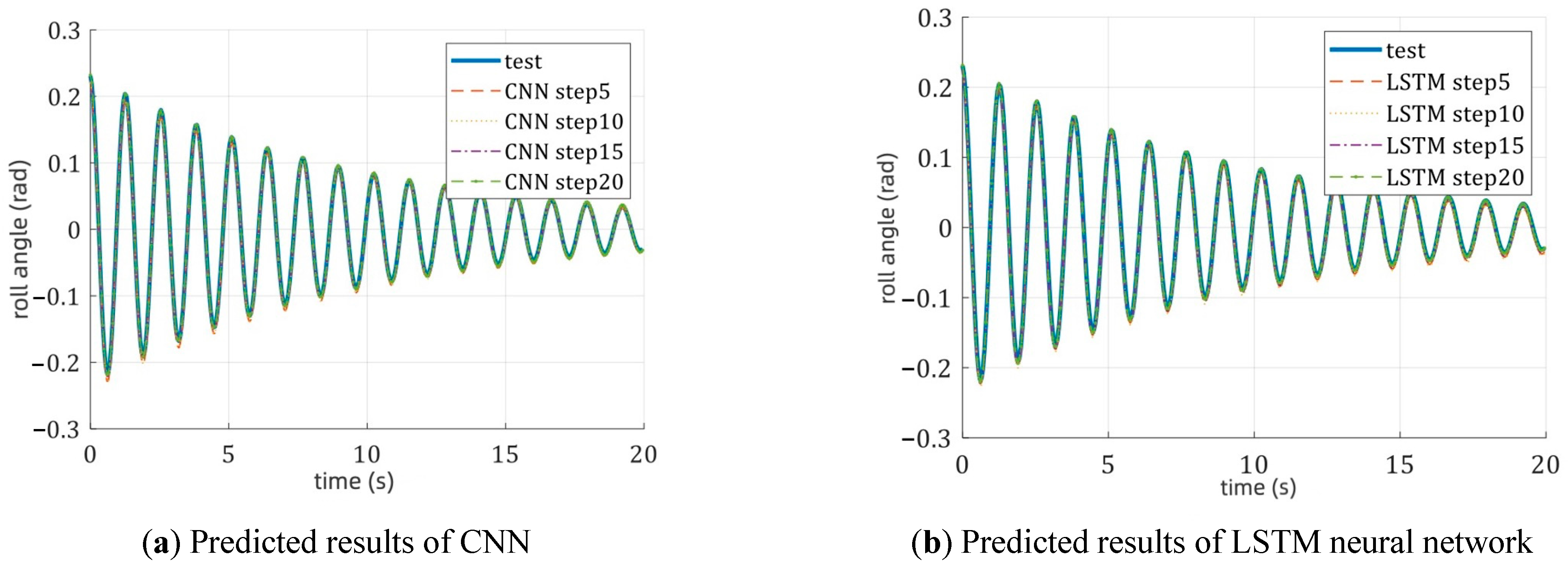
On the basis of the obtained simulation data for the nonlinear roll motion in regular waves, the training set and test set of CNN are constructed according to the format in Table 1 and Table 2. The training set is employed to train CNN, and the training and learning effect is verified by the test set. At the same time, the LSTM neural network is also used to predict the roll motion. The prediction results of the test set by CNN are displayed in Figure 10. Therein, the prediction results of CNN are shown in Figure 12a, and the predicted results of LSTM neural network are shown in Figure 12b.

Table 7. Predicted error of roll motion in regular waves.

	MAE (×10−8)		RMSE (×10−7)		MSE (×10−14)		R2
	CNN	LSTM	CNN	LSTM	CNN	LSTM	CNN	LSTM
1	7.020	1.430	1.027	1.800	1.055	3.238	0.999999961	0.999999882
2	7.350	1.742	1.065	2.204	1.135	4.860	0.999999958	0.999999822
3	7.794	2.134	1.095	2.715	1.200	7.373	0.999999956	0.999999730
4	8.180	2.615	1.118	3.345	1.250	1.119	0.999999954	0.999999590
5	8.611	3.182	1.162	4.088	1.350	1.671	0.999999950	0.999999388

and

Table 8. Prediction error increase of roll motion in regular waves.

	MAE (%)		RMSE (%)		MSE (%)
	CNN	LSTM	CNN	LSTM	CNN	LSTM
1	4.70	21.80	3.70	22.44	7.58	50.09
2	6.04	22.50	2.82	23.19	5.73	51.71
3	4.95	22.53	2.10	23.20	4.17	51.77
4	5.27	21.68	3.94	22.21	8.00	49.33

present the predicted discrepancies between CNN and LSTM neural networks, along with the incremental changes in forecast errors at each step.

According to the above results, it can be seen that both CNN and LSTM can carry out short-term forecasts of ship roll motion in regular waves, and the forecast error increase for CNN is lower than that for LSTM, i.e., the short-term forecast effect for CNN is better than that for LSTM.

5.3. Prediction of Roll Motion in Irregular Waves

In this subsection, regarding the accuracy and applicability of CNN for prediction of the nonlinear roll motion in irregular waves, this paper applies CNN to analyze the random roll motion data excited by six irregular wave spectra, namely white noise spectrum, P-M spectrum, JONSWAP spectrum, Neumann spectrum, ITTC spectrum and dual parameter spectrum. At the same time, the LSTM neural network is also used to predict the nonlinear roll motion excited by the six irregular wave spectra, and the prediction results are compared with that of CNN.

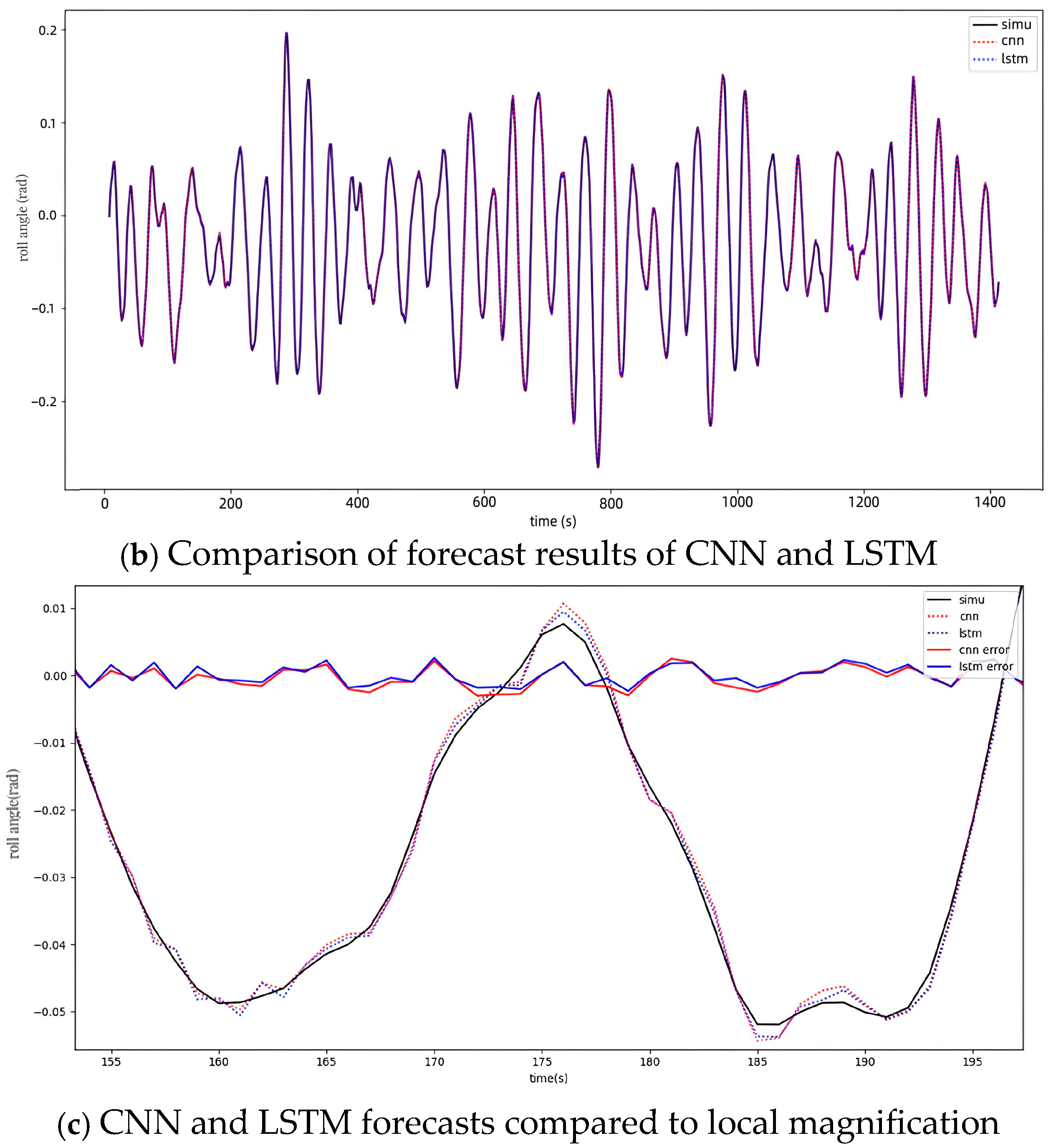
5.3.1. Predicted Results for Roll Motion under White Noise Excitation

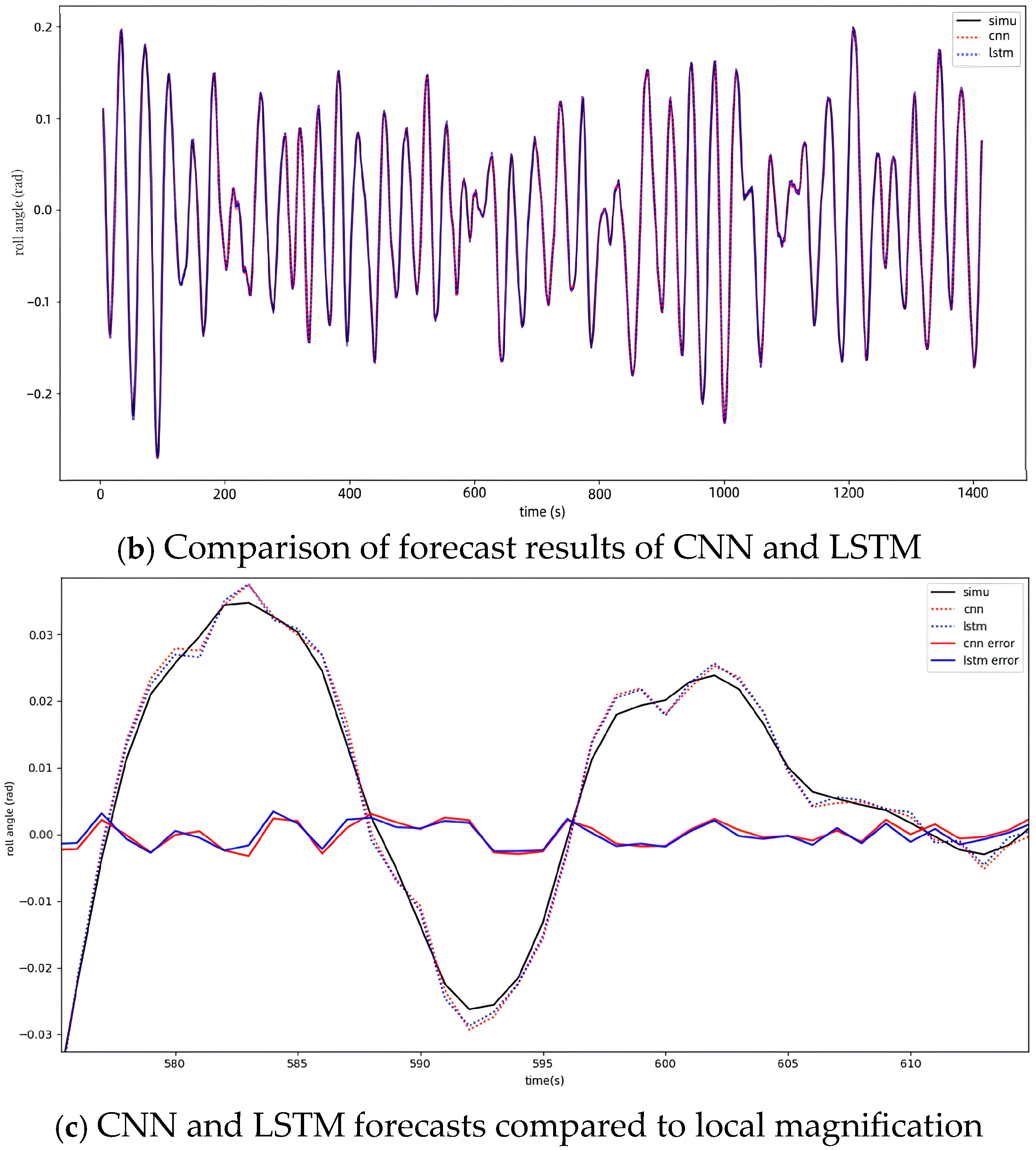
Using CNN and LSTM neural network to predict the nonlinear roll motion excited by the white noise spectrum, the comparison results between CNN and LSTM neural network are shown in Figure 13. Moreover,

Table 9. Predicted errors of roll motion under white noise excitation.

	MAE (×10−2)		RMSE (×10−2)		MSE (×10−4)		R2
	CNN	LSTM	CNN	LSTM	CNN	LSTM	CNN	LSTM
1	0.299	0.388	0.357	0.436	0.128	0.190	0.999251069	0.999495923
2	0.856	1.164	0.989	1.328	0.978	1.763	0.994262024	0.995322706
3	1.488	2.014	1.784	2.414	3.182	5.825	0.981330293	0.984546377
4	2.173	2.963	2.665	3.607	7.100	13.01	0.958345566	0.965479822
5	2.895	3.966	3.569	4.836	12.74	23.38	0.925254810	0.937962555

and

Table 10. Prediction error increase of roll motion under white noise excitation.

	MAE (%)		RMSE (%)		MSE (%)
	CNN	LSTM	CNN	LSTM	CNN	LSTM
1	186.13	200.07	176.77	204.66	665.86	827.89
2	73.87	73.02	80.40	81.78	225.36	230.40
3	46.03	47.12	49.38	49.42	123.13	123.35
4	33.23	33.85	33.92	34.07	79.44	79.71

give the predicted errors of CNN and LSTM under white noise spectrum excitation and the error growth of each step in the five-step prediction.

Combining the prediction comparison in Figure 13 and the predicted evaluation indicators given in Table 9 and Table 10, it can be founded that both models performed well under the four evaluations. The indicators of the CNN model under the four evaluations were smaller than those of the LSTM model, which illustrates that the prediction performance of CNN model is better than that of LSTM model. The error increase at each step in the five-step prediction of the CNN model is lower than that of LSTM, indicating that the CNN model has higher accuracy.

5.3.2. Predicted Results of Roll Motion under P-M Spectrum Excitation

The CNN and LSTM neural network was used to predict the nonlinear roll motion excited by the P-M spectrum, and the comparison results between CNN and LSTM neural networks are shown in Figure 14. Moreover,

Table 11. Predicted errors of roll motion under P-M spectrum excitation.

	MAE (×10−2)		RMSE (×10−2)		MSE (×10−4)		R2
	CNN	LSTM	CNN	LSTM	CNN	LSTM	CNN	LSTM
1	0.315	0.323	0.381	0.394	0.145	0.155	0.999351319	0.999304812
2	0.872	0.870	1.013	1.008	1.026	1.015	0.995404745	0.995453743
3	1.503	1.491	1.812	1.791	3.284	3.206	0.985296580	0.985644504
4	2.199	2.175	2.691	2.657	7.240	7.061	0.967585505	0.968387693
5	2.913	2.887	3.586	3.550	12.86	12.60	0.942431539	0.943579568

and

Table 12. Prediction error increase of roll motion under P-M spectrum excitation.

	MAE (%)		RMSE (%)		MSE (%)
	CNN	LSTM	CNN	LSTM	CNN	LSTM
1	176.74	169.05	166.16	155.84	608.07	553.57
2	72.36	71.36	78.87	77.68	220.08	215.86
3	46.31	45.86	48.51	48.35	120.46	120.24
4	32.47	32.73	33.26	33.61	77.62	78.44

demonstrate the predicted errors of CNN and LSTM under P-M spectrum excitation and the error growth of each step in the five-step prediction.

From the prediction results in Figure 14, Table 11 and Table 12, it can be seen that both models performed well under the four evaluations. The MAE, MSE and RMSE evaluation indicators of the CNN model are smaller than those of the LSTM model, and the R² evaluation index is close to 1, which shows that the CNN model has better prediction performance. The error increase for each step of the CNN is higher than that of the LSTM model. Therefore, the CNN model is more accurate in the short-term prediction of the roll motion excited by the P-M spectrum, and the LSTM model has higher accuracy in the long-term prediction.

5.3.3. Predicted Results of Roll Motion under JONSWAP Spectrum Excitation

Using CNN and LSTM neural network to predict the nonlinear roll motion excited by the JONSWAP spectrum, the comparison results between CNN and LSTM neural networks are shown in Figure 15.

Table 13. Predicted errors for roll motion under JONSWAP spectrum excitation.

	MAE (×10−2)		RMSE (×10−2)		MSE (×10−4)		R2
	CNN	LSTM	CNN	LSTM	CNN	LSTM	CNN	LSTM
1	0.389	0.391	0.433	0.438	0.187	0.192	0.999567844	0.999558655
2	1.175	1.172	1.335	1.332	1.782	1.775	0.995884420	0.995908648
3	2.040	2.034	2.425	2.425	5.879	5.879	0.986422801	0.986448216
4	2.983	2.991	3.624	3.635	13.14	13.22	0.969665359	0.969538313
5	3.994	4.006	4.885	4.908	23.87	24.09	0.944883308	0.944474978

and

Table 14. Prediction error increase for roll motion under JONSWAP spectrum excitation.

	MAE (%)		RMSE (%)		MSE (%)
	CNN	LSTM	CNN	LSTM	CNN	LSTM
1	201.98	196.16	208.60	194.46	852.43	826.89
2	73.62	76.08	81.65	83.72	229.91	231.21
3	46.23	49.14	49.44	51.38	123.51	124.87
4	33.89	35.34	34.80	36.04	81.66	82.22

give the predicted errors of CNN and LSTM under JONSWAP spectrum excitation and the error growth of each step in the five-step prediction.

From Figure 13, Table 13 and Table 14, it can be seen that both models performed well under the four evaluations. The MAE, MSE and RMSE evaluation indicators of the CNN model are smaller than those of the LSTM model, and there is no hysteresis in the prediction curve of the CNN model, which shows that the CNN model has better prediction performance. However, the CNN model has poor prediction results at wave peaks and troughs, indicating that the performance in complex conditions needs to be further improved.

5.3.4. Predicted Results for Roll Motion under Neuman Spectrum Excitation

Using CNN and LSTM neural networks to predict the nonlinear roll motion excited by the Neuman spectrum, the comparison results between CNN and LSTM neural network are shown in Figure 16. Moreover, the predicted errors for CNN and LSTM under Neuman spectrum excitation and the error growth of each step in the five-step prediction are given in

Table 15. Predicted errors for roll motion under Neuman spectrum excitation.

	MAE (×10−2)		RMSE (×10−2)		MSE (×10−5)		R2
	CNN	LSTM	CNN	LSTM	CNN	LSTM	CNN	LSTM
1	0.155	0.156	0.175	0.181	0.308	0.326	0.999608836	0.999585055
2	0.461	0.462	0.532	0.532	2.834	2.828	0.996396982	0.996403677
3	0.810	0.814	0.971	0.977	9.430	9.545	0.988009648	0.987863093
4	1.212	1.214	1.469	1.479	21.58	21.88	0.972564665	0.972178763
5	1.632	1.643	1.992	2.012	39.67	40.48	0.949557517	0.948521252

and

Table 16. Prediction error increase for roll motion under Neuman spectrum excitation.

	MAE (%)		RMSE (%)		MSE (%)
	CNN	LSTM	CNN	LSTM	CNN	LSTM
1	198.06	196.16	203.48	194.46	821.33	766.69
2	75.62	76.08	82.45	83.72	232.75	237.52
3	49.67	49.14	51.26	51.38	128.84	129.23
4	34.65	35.34	35.60	36.04	83.83	85.01

, respectively.

Combining the prediction results in Figure 16 and evaluation indicators shown in Table 15 and Table 16, it can be discerned that both models performed well under the four evaluations. The MSE, MAE and RMSE evaluation indicators for the CNN model are smaller than those for the LSTM model, which shows that the CNN model has better prediction performance. The error increase in each step of the CNN is lower than that of the LSTM model. Therefore, the CNN model is more accurate in the short-term prediction of the roll motion excited by the Neuman spectrum.

5.3.5. Predicted Results of Roll Motion under ITTC Spectrum Excitation

The nonlinear roll motion excited by the ITTC spectrum was predicted by using CNN and LSTM neural networks, and the comparison results between CNN and LSTM neural network are shown in Figure 17.

Table 17. Predicted errors of roll motion under ITTC spectrum excitation.

	MAE (×10−2)		RMSE (×10−2)		MSE (×10−4)		R2
	CNN	LSTM	CNN	LSTM	CNN	LSTM	CNN	LSTM
1	0.393	0.398	0.443	0.448	0.196	0.201	0.999397138	0.999381032
2	1.158	1.156	1.325	1.324	1.756	1.753	0.994592842	0.994601848
3	1.977	1.969	2.375	2.376	5.639	5.648	0.982636877	0.982609198
4	2.885	2.879	3.528	3.532	12.45	12.47	0.961670673	0.961587315
5	3.838	3.826	4.713	4.725	22.22	22.33	0.931586128	0.931242631

and

Table 18. Prediction error increase for roll motion under ITTC spectrum excitation.

	MAE (%)		RMSE (%)		MSE (%)
	CNN	LSTM	CNN	LSTM	CNN	LSTM
1	194.96	190.60	199.44	195.34	796.83	772.14
2	70.73	70.33	79.25	79.46	221.13	222.19
3	45.93	46.22	48.55	48.65	120.78	120.79
4	33.03	32.89	33.59	33.78	78.47	79.07

give the forecast errors for CNN and LSTM under ITTC spectrum excitation and the error growth for each step in the five-step prediction.

From Figure 17, Table 17 and Table 18, it can be discerned that the prediction curves of the CNN and LSTM models are close to the real curves and basically consistent with the trend of the real curves. Both models performed well under the four evaluations. The MSE and RMSE evaluation indicators for the CNN model are smaller than those for the LSTM model, which shows that the CNN model has better prediction performance.

5.3.6. Predicted Results of Roll Motion under Double-Parameter Spectrum Excitation

The nonlinear roll motion excited by the double-parameter spectrum was predicted by, respectively, using the CNN and LSTM neural networks, and the comparison results between CNN and LSTM neural networks are shown in Figure 18. Moreover, the predicted errors for CNN and LSTM under double-parameter spectrum excitation and the error growth for each step in the five-step prediction are given in

Table 19. Predicted errors for roll motion under double-parameter spectrum excitation.

	MAE (×10−2)		RMSE (×10−2)		MSE (×10−5)		R2
	CNN	LSTM	CNN	LSTM	CNN	LSTM	CNN	LSTM
1	0.145	0.144	0.166	0.162	0.274	0.262	0.999648903	0.999664904
2	0.434	0.430	0.501	0.492	2.514	2.418	0.996784415	0.996905922
3	0.762	0.752	0.916	0.901	8.387	8.102	0.989270467	0.989631827
4	1.124	1.110	1.377	1.359	18.95	18.48	0.975760027	0.976351532
5	1.508	1.492	1.861	1.844	34.64	34.00	0.955680647	0.956495798

and

Table 20. Prediction error increase for roll motion under double-parameter spectrum excitation.

	MAE (%)		RMSE (%)		MSE (%)
	CNN	LSTM	CNN	LSTM	CNN	LSTM
1	199.72	198.40	202.60	203.89	816.18	823.25
2	75.65	74.77	82.65	83.06	233.61	235.07
3	47.45	47.70	50.36	50.98	125.95	128.09
4	34.16	34.41	35.15	35.69	82.80	83.98

, respectively. From Figure 18, Table 19 and Table 20, it can be clearly seen that both models performed well under the four evaluations. It can be seen from the evaluation index that the performance of the LSTM model is better than that of the CNN model. The CNN model’s short-term accuracy in predicting the roll motion under double-parameter spectrum excitation is lower than that of the LSTM model, but it can still meet expectations.

Through the above analysis, it can be seen that CNN can achieve accurate prediction of roll motion through learning from the simulation data under external excitation of six irregular spectra, respectively. Moreover, the comparison results demonstrate that CNN has the same prediction precision as that of LSTM neural network. Considering that, in the field of ship motion prediction, irregular waves are mainly approximated by the above six irregular wave spectra, the research results may demonstrate that CNN can be used to predict the nonlinear roll motion in the short term at sea.

6. Conclusions

In this study, CNN is applied to predict the roll motion of ships in the short term. In order to validate the applicability and effectiveness of CNN in the prediction of ship roll motion, free roll decay motion in still water, roll motion in regular waves, and irregular roll motion under excitations of six different wave spectra are predicted, respectively. Meanwhile, the prediction results of CNN are compared with those of LSTM neural network. The comparison results demonstrate that CNN can be applied to predict the roll motion accurately, and it has the same prediction accuracy as that of LSTM neural network. With reasonable training, the model can predict complex nonlinear phenomena. Moreover, this method is not limited by the physical model and has strong prediction performance.

In the present study, only the simulated historical data of ship roll motion is considered as the learning samples set. However, the ship usually suffers from six degree of freedom oscillating motion during navigation, and the measured historical motion data is contaminated by different levels of noise. The efficiency and robustness of the proposed prediction model can be improved by incorporating more useful information. In this paper, the authors focused on the application of CNN to the analysis of ship real multi-freedom measurement data.

References

1. Wang, Y.; Wang, H.; Zhou, B.; Fu, H. Multi-Dimensional Prediction Method Based on Bi-LSTMC for Ship Roll. Ocean Eng. 2021, 242, 110106. [Google Scholar] [CrossRef]
2. Hashimoto, H.; Omura, T.; Matsuda, A.; Yoneda, S.; Stern, F.; Tahara, Y. Several Remarks on EFD and CFD for Ship Roll Decay. Ocean Eng. 2019, 186, 106082. [Google Scholar] [CrossRef]
3. Kianejad, S.S.; Enshaei, H.; Duffy, J.; Ansarifard, N. Calculation of Ship Roll Hydrodynamic Coefficients in Regular Beam Waves. Ocean Eng. 2020, 203, 107225. [Google Scholar] [CrossRef]
4. Kianejad, S.S.; Enshaei, H.; Duffy, J.; Ansarifard, N.; Ranmuthugala, D. Ship Roll Damping Coefficient Prediction Using CFD. Ocean Eng. 2019, 63, 108–122. [Google Scholar] [CrossRef]
5. Liu, L.W.; Chen, M.X.; Wang, X.Z.; Zhang, Z.G.; Yu, J.W.; Feng, D.K. CFD prediction of full-scale ship parametric roll in head wave. Ocean Eng. 2021, 233, 109180. [Google Scholar] [CrossRef]
6. Chen, C.; Liu, Y.D.; Zhang, W.; He, Y.P.; Tang, Y.Y. Free roll decay simulation of a polar research vessel with an anti-roll tank based on CFD. Ocean Eng. 2023, 285, 115429. [Google Scholar] [CrossRef]
7. Jiang, H.; Duan, S.; Huang, L.; Han, Y.; Yang, H.; Ma, Q. Scale Effects in AR Model Real-Time Ship Motion Prediction. Ocean Eng. 2020, 203, 107202. [Google Scholar] [CrossRef]
8. Selvaraj, J.J.; Arunachalam, V.; Coronado-Franco, K.V.; Romero-Orjuela, L.V.; Ramírez-Yara, Y.N. Time-Series Modeling of Fishery Landings in the Colombian Pacific Ocean Using an ARIMA Model. Reg. Stud. Mar. Sci. 2020, 39, 101477. [Google Scholar] [CrossRef]
9. Yin, J.-C.; Perakis, A.N.; Wang, N. A Real-Time Ship Roll Motion Prediction Using Wavelet Transform and Variable RBF Network. Ocean Eng. 2018, 160, 10–19. [Google Scholar] [CrossRef]
10. Huang, B.-G.; Zou, Z.-J.; Ding, W.-W. Online Prediction of Ship Roll Motion Based on a Coarse and Fine Tuning Fixed Grid Wavelet Network. Ocean Eng. 2018, 160, 425–437. [Google Scholar] [CrossRef]
11. Chen, C.; Ruiz, M.T.; Delefortrie, G.; Mei, T.; Vantorre, M.; Lataire, E. Parameter Estimation for a Ship’s Roll Response Model in Shallow Water Using an Intelligent Machine Learning Method. Ocean Eng. 2019, 191, 106479. [Google Scholar] [CrossRef]
12. Suhermi, N.; Suhartono; Prastyo, D.D.; Ali, B. Roll Motion Prediction Using a Hybrid Deep Learning and ARIMA Model. Procedia Comput. Sci. 2018, 144, 251–258. [Google Scholar] [CrossRef]
13. Xue, L.; Wu, H.; Zheng, H.; He, Z. Control Chart Pattern Recognition for Imbalanced Data Based on Multi-Feature Fusion Using Convolutional Neural Network. Comput. Ind. Eng. 2023, 182, 109410. [Google Scholar] [CrossRef]
14. Belomestny, D.; Naumov, A.; Puchkin, N.; Samsonov, S. Simultaneous Approximation of a Smooth Function and Its Derivatives by Deep Neural Networks with Piecewise-Polynomial Activations. Neural Netw. 2023, 161, 242–253. [Google Scholar] [CrossRef] [PubMed]
15. Rithani, M.; Kumar, R.P.; Doss, S. A Review on Big Data Based on Deep Neural Network Approaches. Artif. Intell. Rev. 2023, 56, 14765–14801. [Google Scholar] [CrossRef]
16. Hochreiter, S.; Schmidhuber, J. Long Short-Term Memory. Neural Comput. 1997, 9, 1735–1780. [Google Scholar] [CrossRef] [PubMed]
17. Zhang, T.; Zheng, X.-Q.; Liu, M.-X. Multiscale Attention-Based LSTM for Ship Motion Prediction. Ocean Eng. 2021, 230, 109066. [Google Scholar] [CrossRef]
18. Zhang, D.; Zhou, X.; Wang, Z.-H.; Peng, Y.; Xie, S.-R. A Data Driven Method for Multi-Step Prediction of Ship Roll Motion in High Sea States. Ocean Eng. 2023, 276, 114230. [Google Scholar] [CrossRef]
19. Chen, Z.; Zhao, C.; Tu, Y.; Chen, X.; Yang, R. A BiLSTM Hybrid Model for Ship Roll Multi-Step Forecasting Based on Decomposition and Hyperparameter Optimization. Ocean Eng. 2021, 242, 110138. [Google Scholar]
20. Jiang, Y.; Hou, X.-R.; Wang, X.-G.; Wang, Z.-H.; Yang, Z.-L.; Zou, Z.-J. Identification Modeling and Prediction of Ship Maneuvering Motion Based on LSTM Deep Neural Network. J. Mar. Sci. Technol. 2022, 27, 125–137. [Google Scholar] [CrossRef]
21. Wang, Y.-C.; Wang, H.; Zou, D.-X.; Fu, H.-X. Ship Roll Prediction Algorithm Based on Bi-LSTM-TPA Combined Model. J. Mar. Sci. Eng. 2021, 9, 387. [Google Scholar] [CrossRef]
22. Sun, Q.; Tang, Z.; Gao, J.; Zhang, G. Short-Term Ship Motion Attitude Prediction Based on LSTM and GPR. Appl. Ocean Res. 2022, 118, 102927. [Google Scholar] [CrossRef]
23. Xu, Q.; Yang, Y.; Zhang, C.; Zhang, L. Deep Convolutional Neural Network-Based Autonomous Marine Vehicle Maneuver. Int. J. Fuzzy Syst. 2018, 20, 687–699. [Google Scholar] [CrossRef]
24. Zhou, J.; Ren, K.; Wan, M.; Cheng, B.; Gu, G.; Chen, Q. An Infrared and Visible Image Fusion Method Based on VGG-19 Network. Optik 2021, 248, 168084. [Google Scholar] [CrossRef]
25. Ak, A.; Topuz, V.; Midi, I. Motor Imagery EEG Signal Classification Using Image Processing Technique over GoogLeNet Deep Learning Algorithm for Controlling the Robot Manipulator. Biomed. Signal Process. Control 2022, 72, 103295. [Google Scholar] [CrossRef]
26. Jiang, Y.; Li, Y.; Zhang, H. Hyperspectral Image Classification Based on 3-D Separable ResNet and Transfer Learning. IEEE Geosci. Remote Sens. Lett. 2019, 16, 1949–1953. [Google Scholar] [CrossRef]
27. Alexandersson, M.; Mao, W.; Ringsberg, J.W. Analysis of Roll Damping Model Scale Data. Ships Offshore Struct. 2021, 16, 85–92. [Google Scholar] [CrossRef]
Figure 1. Convolutional neural network.
Jmse 12 00102 g001
Figure 2. Brief flow chart of CNN.
Jmse 12 00102 g002
Figure 3. Free roll decay motion.
Jmse 12 00102 g003
Figure 4. Roll motion under regular wave conditions.
Jmse 12 00102 g004
Figure 5. White noise spectral roll angle simulation.
Jmse 12 00102 g005
Figure 6. P-M spectral roll angle simulation.
Jmse 12 00102 g006
Figure 7. JONSWAP spectral roll angle simulation.
Jmse 12 00102 g007
Figure 8. Neuman spectral roll angle simulation.
Jmse 12 00102 g008
Figure 9. ITTC spectral roll angle simulation.
Jmse 12 00102 g009
Figure 10. Two-parameter spectral roll angle simulation.
Jmse 12 00102 g010
Figure 11. Predicted results for free roll decay motion.
Jmse 12 00102 g011
Figure 12. Predicted results of roll motion in regular waves.
Jmse 12 00102 g012
Figure 13. Predicted results of roll motion under white noise excitation.
Jmse 12 00102 g013
Figure 14. Predicted results of roll motion under P-M spectrum excitation.
Jmse 12 00102 g014aJmse 12 00102 g014b
Figure 15. Predicted results of roll motion under JONSWAP spectrum excitation.
Jmse 12 00102 g015
Figure 16. Predicted results for roll motion under Neuman spectrum excitation.
Jmse 12 00102 g016aJmse 12 00102 g016b
Figure 17. Predicted results of roll motion under ITTC spectrum excitation.
Jmse 12 00102 g017
Figure 18. Predicted results for roll motion under double-parameter spectrum excitation.
Jmse 12 00102 g018aJmse 12 00102 g018b