Article

A Machine-Learning Approach Based on Attention Mechanism for Significant Wave Height Forecasting

1
Key Laboratory of Marine Geology and Metallogeny, First Institute of Oceanography, Ministry of Natural Resources, Qingdao 266061, China
2
Laboratory for Regional Oceanography and Numerical Modeling, Pilot National Laboratory for Marine Science and Technology (Qingdao), Qingdao 266061, China
3
National Engineering Laboratory for Integrated Aero-Space-Ground-Ocean Big Data Application Technology, Qingdao 266061, China
4
Key Laboratory of Marine Environmental Science and Numerical Modelling, First Institute of Oceanography, Ministry of Natural Resources, Qingdao 266061, China
*
Author to whom correspondence should be addressed.
J. Mar. Sci. Eng. 2023, 11(9), 1821; https://doi.org/10.3390/jmse11091821
Submission received: 7 August 2023 / Revised: 1 September 2023 / Accepted: 5 September 2023 / Published: 19 September 2023

Abstract

:
Significant wave height (SWH) is a key parameter for monitoring the state of waves. Accurate and long-term SWH forecasting is significant to maritime shipping and coastal engineering. This study proposes a transformer model based on an attention mechanism to achieve the forecasting of SWHs. The transformer model can capture the contextual information and dependencies between sequences and achieves continuous time series forecasting. Wave scale classification is carried out according to the forecasting results, and the results are compared with gated recurrent unit (GRU) and long short-term memory (LSTM) machine-learning models and the key laboratory of MArine Science and NUmerical Modeling (MASNUM) numerical wave model. The results show that the machine-learning models outperform the MASNUM within 72 h, with the transformer being the best model. For continuous 12 h, 24 h, 36 h, 48 h, 72 h, and 96 h forecasting, the average mean absolute errors (MAEs) of the test sets were, respectively, 0.139 m, 0.186 m, 0.223 m, 0.254 m, 0.302 m, and 0.329 m, and the wave scale classification accuracies were, respectively, 91.1%, 99.4%, 86%, 83.3%, 78.9%, and 77.5%. The experimental results validate that the transformer model can achieve continuous and accurate SWH forecasting, as well as accurate wave scale classification and early warning of waves, providing technical support for wave monitoring.

1. Introduction

Marine forecasting plays an extremely important role in supporting coastal engineering construction, disaster prevention and mitigation, marine ecological civilization construction, and economic development. Forecasting significant wave height (SWH) holds important scientific value for monitoring the state of waves [1,2,3,4,5,6].
Traditional numerical models for wave forecasting are based on physical dynamics, solving a wave action balance equation through the use of discrete calculations [1]. However, these models are usually computationally expensive and complex [1,2]. In contrast, existing machine-learning methods focus on data association and do not rely on physical mechanisms. Compared to numerical models, existing machine-learning methods offer lower computational and time costs and achieve higher accuracy in short-term wave forecasting [3,4,5,6,7,8,9,10,11,12,13,14,15,16,17,18,19,20,21,22,23,24,25]. Commonly used machine-learning models for wave forecasting include artificial neural network (ANN) [3], backpropagation (BP) [4], support vector machine (SVM) [5,6,7], long short-term memory (LSTM) [8,9,10,11,12,13,14,15,16,17], bidirectional LSTM (BiLSTM) [18,19,20], gated recurrent unit (GRU) [17,21,22,23], and bidirectional GRU (BiGRU) [24,25]. These models capture the envolution of wave height with time from historical information or model wave envolution based on the driving effect from the wind and the influences of other environmental features (e.g., air pressure and temperature) on waves. Wave forecasting is divided into point-to-point forecasting and continuous-sequence forecasting. Most current studies focus on point-to-point forecasting, where waves at specific time steps in the future are forecasted by setting the length of the forecast window. Prahlada et al. [3] utilized a hybrid model, combining wavelet analysis and an artificial neural network (WLNN) to forecast the significant wave height in a time series, with lead times extending up to 48 h. The root mean square error (RMSE) for a 48 h forecast horizon near the western region of Eureka, Canada, in the North Pacific Ocean was found to be 1.076 m. Under normal conditions, the mean absolute percentage error (MAPE) for a 12 h forecast was 61%, while under extreme conditions, it reduced to 40%. Li et al. [21] used a GRU model and introduced environmental features such as wind speed and sea temperature to predict SWH 1–3 h ahead. Wave height data were collected from six monitoring stations in the offshore waters of China. Zhou et al. [9] used a convolutional LSTM (ConvLSTM) model to perform forecasting 3–24 h ahead using National Oceanic and Atmospheric Administration (NOAA) wave reanalysis data under normal and extreme weather conditions. The mean absolute percentage error (MAPE) of a 12 h forecast was 61% under normal conditions and 40% under extreme conditions.
In addition to using machine-learning models for short-term forecasting, some studies [8,18,19,20,26] have found that the combination of attention mechanisms or decomposition methods with machine-learning algorithms can greatly improve SWH forecasting. In a study by Zhou et al. [8], an integrated model combining empirical mode decomposition (EMD) and LSTM was employed for forecasting SWH in the Atlantic Ocean at 3, 6, 12, 24, 48, and 72 h horizons. Wang et al. [19] proposed a convolutional neural network (CNN)–BiLSTM–attention model and used it to carry out SWH forecasting 1–24 h ahead under normal and typhoon conditions using WaveWatch III (WW3) reanalysis data from the East China Sea and South China Sea from 2011 to 2020. The average RMSEs for the forecasts at 3, 6, 12, and 24 h were observed to be 0.063 m, 0.105 m, 0.172 m, and 0.281 m, respectively, under normal conditions. Under extreme conditions, the corresponding RMSEs were 0.159 m, 0.257 m, 0.437 m, and 0.555 m. Notably, this model outperformed the one trained solely on WW3 reanalysis data. The results demonstrate that the incorporation of an attention mechanism improved the forecasting accuracy of the model. Celik [26] constructed a hybrid model by integrating an adaptive neuro-fuzzy inference system (ANFIS) with singular value decomposition (SVD) for forecasting SWH in the Pacific and Atlantic Oceans at lead times ranging from 1 to 24 h.
Single-time forecasting can provide high-accuracy SWH forecasts at a specific time. There are two methods for observing continuous SWH envolution over a period of time in the future. One method involves establishing multiple single-time models, which requires considerable computational cost. The other method is to build a time series forecasting model, which may sacrifice the accuracy of forecasting at individual points but save computational cost and can provide an accurate forecast trend. In recent years, the attention-mechanism-based transformer model [27] has attracted attention due to its excellent performance in time series forecasting tasks. This model was initially proposed by the Google team in 2017 for natural language-processing (NLP) applications. Since then, it has been gradually optimized and is widely used in speech recognition [28], computer vision [29], time series forecasting [30,31], anomaly detection [32,33], and other fields [34]. Researchers in the marine field have noted the advantages of the transformer model and applied it to marine time series data forecasting [35,36,37,38,39]. Immas et al. [35] used both LSTM and transformer to achieve real-time in situ forecasting of ocean currents. The two models performed similarly and provided valuable guidance for the path planning of autonomous underwater vehicles. Zhou et al. [36] developed a 3D-geoformer model based on the transformer model to forecast El Niño 3.4 sea surface temperature (SST) anomalies 18 months in advance, achieving a Pearson correlation coefficient of 50%. Their results were comparable to those of Ham et al. [40], who used a CNN to forecast El Niño/southern oscillation. Feng et al. [37] used a transformer model to forecast the El Niño index, and the results were better than those using a CNN. Pokhrel et al. [38] proposed differencing SWHs fitted with WW3 and measured data and used a transformer model to forecast residuals at specific time steps. Compared to WW3 predictions, the transformer-network-based residual correction for a 3 h forecast provided more accurate estimations. The results showed that the combination of numerical modeling and artificial intelligence algorithms yields a better performance.
Currently, there are very limited applications of transformer models in continuous wave forecasting [38,41] and wave scale classification. To fill this research gap, in this study, an attempt is made to use an attention-mechanism-based transformer model to achieve sequence-to-sequence learning for SWH. This model extracts the driving effects of various features on the SWH evolution from the historical information of input features, captures the contextual information and dependencies between sequences, and achieves continuous SWH forecasting, allowing the overall trend of wave changes in the future to be monitored and providing technical support for wave warning and forecasting.
The remainder of this paper is structured as follows. Section 2 describes the data used, Section 3 introduces the methods and experimental setup employed in this study, Section 4 analyzes the results, and Section 5 summarizes the findings.

2. Materials

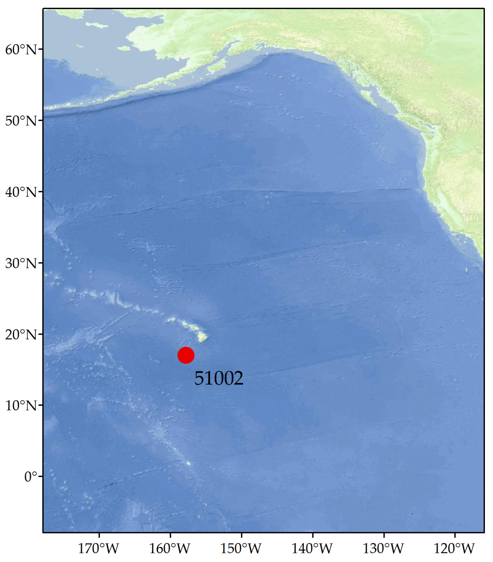
2.1. Experimental Data

Li et al. [42] showed that the wave field in the Pacific Ocean is characterized by clear seasonal variations, with higher wave heights in winter and lower wave heights in summer. Swells dominate in mixed waves. Influenced by the westerly wind belt, there is a relatively large wind and wave intensity for all seasons, reaching approximately 1 m in the central Pacific Ocean north of the equator (near the Hawaiian Islands). The waves in this area have strong nonstationarity and a random nature, making it challenging to fit their envolution accurately. In this study, a buoy deployed by the NOAA in the waters southwest of the Hawaiian Islands in the central North Pacific Ocean was chosen as the research object, as the buoy provides relatively complete hourly ocean data. The geographical location of the buoy is shown in Figure 1, and specific details are provided in Table 1. Liu et al. [43] conducted an analysis of meteorological data pertaining to shipping in the North Pacific Ocean from 1950 to 1995. The data were resolved at a 5° × 5° resolution and revealed that the waves in the equatorial zone predominantly travel in a northeast direction throughout the year. Due to the serious lack of wave direction data of the buoy, Figure 2 only presents the wind rose and wave rose drawn by the buoy data from 2015 to 2022. The larger the radius of the rose, the higher the frequency of occurrence. It is evident from the charts that the prevailing wind direction in this area is east-northeast and east, corresponding to the direction of the waves as well.
Buoy data with a time resolution of 1 h can be obtained from the official website of the U.S. National Data Buoy Center (NDBC) at https://www.ndbc.noaa.gov/ (accessed on 15 May 2023). In this study, the data from 2000 to 2018 were selected as the training set, the data from October 2019 to December 2021 were used as the validation set, and the data from 2022 were used as the test set. The samples were divided using the sliding method, and feature data of the past 96 h were used as input to forecast the SWH for continuous 12 h, 24 h, 36 h, 48 h, 72 h, and 96 h in the future. Due to reasons such as equipment maintenance and sensor malfunctions, the data for some years were missing. Therefore, the original data needed to be cleaned as follows: only continuous valid data were extracted during the training, and data with large portions of consecutive missing data were removed. In cases where there were isolated missing values in the continuous data, linear interpolation was performed to fill in the gaps. The SWH maximum, minimum, average, and variance after data cleaning are shown in Table 2. The numbers of valid samples in the training, validation, and test sets are shown in Table 3.

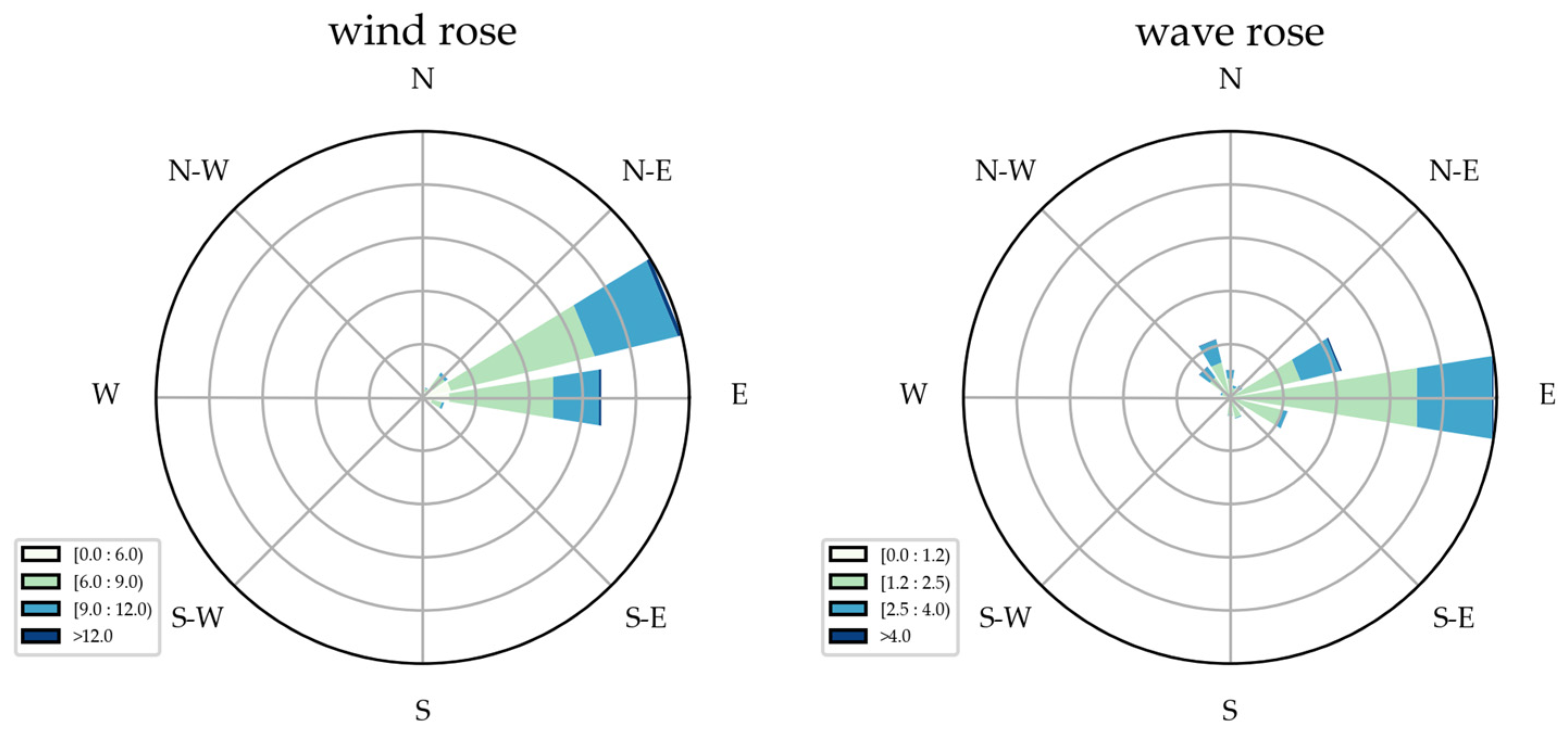
2.2. Feature Selection

Feature selection is a key step in time series forecasting. The buoy data collected by the NDBC included wave information, wind field information, and other environmental features. Wave information consisted of SWH, dominant wave period (DPD), and average wave period (APD); wind field information included wind speed (WSPD), wind direction (WDIR), and peak 5 or 8 s gust speed (GST); and environmental information was composed of air temperature (ATMP), sea surface temperature (WTMP), and sea level pressure (PRES). After data cleaning, a correlation analysis was performed on all buoy feature data by calculating the Pearson correlation coefficients between the features. The results are shown in Figure 3.
Figure 3 shows that SWH had correlation coefficients greater than 0.5 with both WSPD and GST, a weak positive linear correlation with APD and PRES, no clear relationship with wind direction, and a weak negative linear correlation with sea surface temperature and air temperature. In a comprehensive simulation framework examining the evolution of waves, Allahdadi et al. [44] conducted an empirical investigation on various whitecapping formulas. They observed a notable association between the underestimation of wave height and negative values of the air–sea surface temperature difference (dT) at NDBC 44011. Wave change is a complex, dynamic process that is not only related to wind field information and wave information but is also regulated by sea surface temperature and air temperature, although SWH is negatively related to sea surface temperature and air temperature. Therefore, all data mentioned above were combined as input features for training.

2.3. Data Preprocessing

When considering different value ranges and scales (i.e., dimensions) of different feature data, to eliminate the influence of different dimensions on the model training, data preprocessing should be performed before training the model by normalizing different features and scaling the data. The data processing was conducted in this study using min-max normalization, which scales each feature proportionally to a range of [0, 1] using Equation (1) [21]:
x ^ i = x i min ( x i ) max ( x i ) min ( x i )
where x ^ i is the normalized value of x i , max ( x i ) is the maximum value among all x i , and min ( x i ) is the minimum value among all x i .

2.4. Wave Scale Classification Criteria

According to the wave scale level table in the specifications for oceanographic surveys [45] and the SWH changes of the selected buoy, the studied waves were divided into four levels: (i) slight sea: 0   m < H s < 1.25   m ; (ii) moderate sea: 1.25   m H s < 2.5   m ; (iii) rough sea: 2.5   m H s < 4   m ; and (iv) very rough sea: 4   m H s < 6   m . The data volume proportions for these wave scale levels were 0.845%, 64.842%, 33.086%, and 1.227%, respectively. Based on these results, the waves near the Hawaiian Islands are dominated by the moderate and large sea levels.

3. Methodology

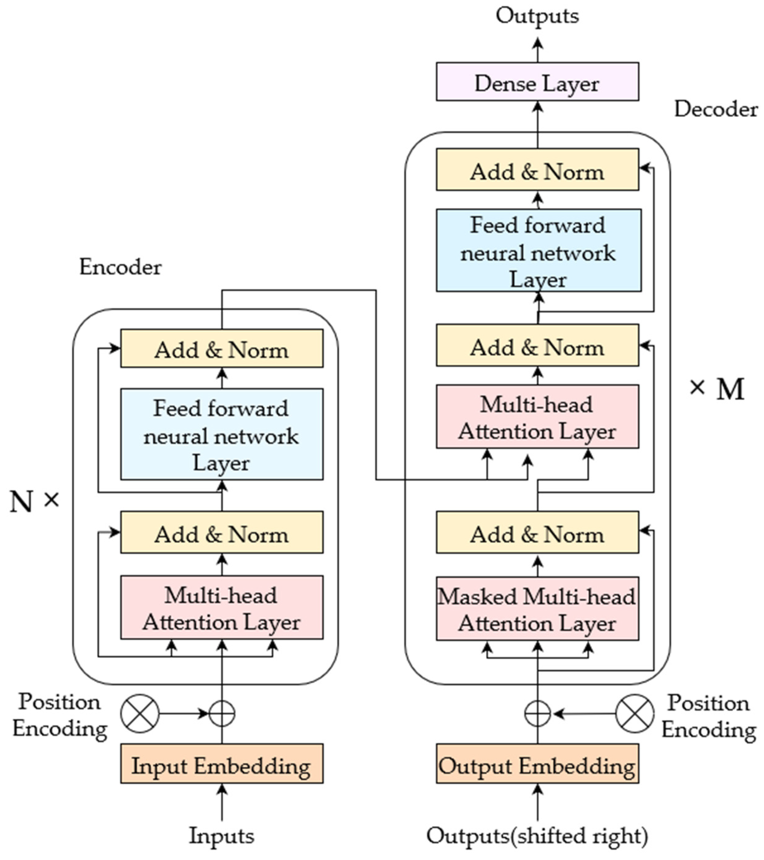
3.1. Model Structure

The structure of the transformer model is shown in Figure 4. The transformer model adopted an “Encoder–Decoder” architecture. The encoder was used to map the input sequence into a high-dimensional space and extract the dependencies of long input sequences, and the decoder was responsible for generating the target sequence. The transformer model was composed of multiple encoder or decoder stacks. An encoder stack contained a multihead attention layer and a feedforward neural network layer, and a decoder stack consisted of two multihead attention layers and a feedforward neural network layer. Residual connections and layer normalization were applied to the output sequences of each layer. Residual connections allowed the model to pass information across multiple layers, while layer normalization sped up the model training and improved the model generalizability. Vaswani et al. [27] proposed a transformer model that employed a learned linear transformation and softmax function to predict the probabilities of subsequent tokens in the decoding process. To map the decoder’s output to the target sequence, a fully connected layer was utilized as the output layer in this study. To assess the impact of encoder and decoder stack numbers on predictions across different time intervals, trials were conducted employing varied numbers ranging from 1 to 6 for both components. The optimal combination selected is presented in Table 4. As the forecasting time increased, the number of layers in the transformer model increased, which was beneficial for capturing long-term dependencies.
The transformer model captured the relationships between the information at different positions in the input sequence through the multihead attention layer and transferred the contextual information of the input sequence to the output sequence. The core of the multihead attention layer was the attention mechanism. The attention mechanism in the transformer model calculated the correlations between the features of the input sequence at different time steps and dynamically assigned weights to the features according to their importance for the output result at each time step, thereby effectively learning the dependencies between the sequence data and helping the model to improve its ability to capture crucial information. The attention weight was calculated using Equation (2) [27]:
Attention ( K , Q , V ) = softmax ( Q K T d k ) V
where Q, K, and V are obtained by mapping the input sequence to different spaces. Here, d k represents the dimension of K. The multihead attention layer mapped the input sequence into h feature subspaces, i.e., h attention heads. Each feature subspace could learn a set of attention weights, and the weight parameters were not shared between subspaces. In addition, various feature subspaces could be processed in parallel, enriching the diversity of feature subspaces without incurring additional computational cost. The multihead attention layer was calculated with Equations (3)–(5) [27]:
Q i = X W Q i , K i = X W K i , V i = X W V i
H i = A t t e n t i o n ( Q i , K i , V i ) , i = 1 , 2 , , h
M u l t i H e a d ( Q , K , V ) = C o n c a t ( H 1 , H 2 , H h ) W O
where W Q i , W K i , and W V i are the linear projection matrices that map the input sequence X to Q, K, and V, respectively, and Hi represents the attention weight of the ith feature subspace.
It can be observed from the calculation equations of the attention mechanism that the attention score of the current position did not depend on the information from the previous time step. Although both the encoding and decoding processes used a multihead attention layer, they differed in their approaches. The attention calculation was bidirectional in the encoding process. However, masking was applied in the decoding process to prevent the model from accessing future information. Thus, the attention mechanism could only focus on the earlier information, enabling the transformer model to be trained in parallel during the encoding process. In the multihead attention layers in both the encoder and decoder, h = 8 [27], the number of neurons in the feedforward neural network layer was set to 2048, and the number of neurons in the final output layer was equal to the number of input features in the model.
The attention mechanism realized the parallel processing of input sequences in the transformer model. However, it did not consider the positional relationships between sequence data. Therefore, before the input sequences were fed into the transformer encoder and decoder, positional encoding was applied to introduce temporal information. Positional encoding refers to an encoding approach in the literature [27] that achieves relative positional encoding using trigonometric functions, as shown in Equation (6).
{ p k , 2 i = s i n ( k 10 , 00 0 2 i / d ) p k , 2 i + 1 = c o s ( k 10 , 00 0 2 i / d )
where p k , 2 i and p k , 2 i + 1 are the (2i)th and (2i + 1)th components of the encoded vector at position k, respectively.
In this study, to maintain the consistency of the input sequence dimension, the original data were linearly embedded using the fully connected layer and combined with the positional encoding results to obtain the final input sequence for the encoder. Here, the number of neurons in the fully connected layer was set to 512 [27].

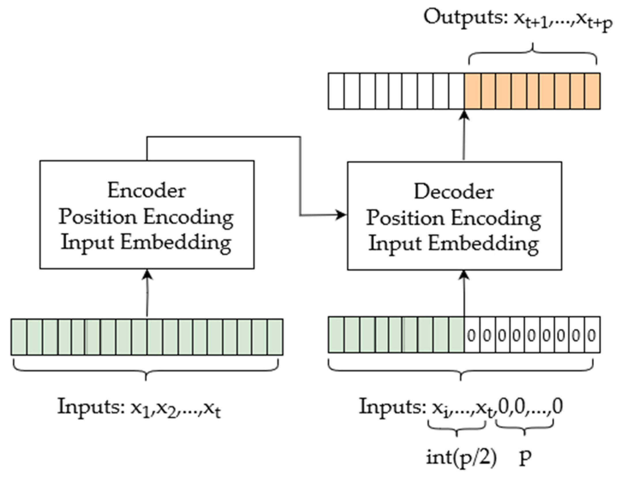
3.2. Introduction of the Output Method

The input of a traditional transformer model [27] is historical features, and various feature results for the next time step are output. To achieve continuous SWH forecasting, an iterative approach is required, which is inefficient and time-consuming. Therefore, we referred to the generative inference in the literature [30], which generates all the results for the forecasted time steps in one forward step. The specific input and output formats are shown in Figure 5.

3.3. Parameter Settings

During model training, a model may overfit the training data due to noise interference caused by redundant data, a complex model structure, and unbalanced training samples. Therefore, a dropout [46] technique is employed to prevent model overfitting. In this study, the dropout parameters were tested between 0.01, 0.02, 0.05, and 0.1, and 0.05 was eventually selected for the encoder and decoder. During backpropagation for parameter optimization, the model used Adam [47] as the optimizer, with a learning rate of 0.0001 [31]. The training batch size for input sequences was selected from 32, 64, and 128, with the best result being 64, and the model was trained for 20 epochs.
To verify the effectiveness of the transformer model, we chose the GRU [48] and LSTM [49] methods as comparative machine-learning models, both of which are commonly used for time series forecasting. The GRU and LSTM used in this study each consisted of a hidden layer, a dropout layer, and a fully connected layer. For both models, the number of neurons in the hidden layer was set to 64, and the number of neurons in the fully connected layer was 16. The other related parameters of the GRU and LSTM were set to be consistent with those of the transformer model.
All three models used the mean squared error (MSE) as the loss function for model training, as shown in Equation (7):
M S E = 1 N i = 1 N ( x i x ^ i ) 2
where N is the number of samples, x i is the true value, and x ^ i is the forecasted value.

3.4. MASNUM Ocean Wave Numerical Model

In this study, the baseline numerical model selected is the key laboratory of MArine Science and NUmerical Modeling (MASNUM) numerical wave model, as proposed by Yang et al. [50]. The governing equation of MASNUM is described by a wave energy spectrum equation and calculated using a complex characteristic inlaid scheme based on the spherical coordinate system. These equations consider the wave–current interaction source function, as well as the wave propagation and refraction along the great circle. MASNUM has been extensively validated and has shown excellent capability in accurately simulating the global distribution of and variations in ocean waves. Hence, it serves as a suitable choice for our baseline model in this study.
The wave energy spectrum balance equation used in the MASNUM numerical model is shown in Equation (8) [50]:
E t + ( C g λ + U λ R c o s φ ) E φ ( C g φ + U φ ) t a n φ R E = S i n + S d s + S b s + S n l + S c u
where E = E ( K , λ , φ , t ) is the wave number spectrum. K = ( k λ , k φ ) is the wave vector, λ is longitude, and φ is latitude. U = ( U λ , U φ ) is the surface current velocity. C g = ( C g λ , C g φ ) is the vector of group velocity. S i n , S d s , S b s , S n l , and S c u are, respectively, the wind input term, wave-breaking term, bottom friction term, wave–wave nonlinear interaction term, and wave–current interaction function. More details can be found in [50].
For the driving wind field of the MASNUM numerical model, we utilized the global meteorological forecast data from the Global Forecast System (GFS) provided by the National Centers for Environmental Prediction (NCEP). The wind field data had a spatial resolution of 0.25° and a temporal resolution of 3 h. The simulation domain covered latitude and longitude ranges from 180° W to 180° E and from 70° S to 70° N. As for the predicted wave field, its spatial resolution was set at 0.25° × 0.25°, with a temporal resolution of 1 h. The numerical integration time for this study spanned from 1 January to 31 December 2022.

3.5. Evaluation Metrics

To assess the performance of our model and compare it with that of the GRU, LSTM, and MASNUM numerical models, we chose mean bias, mean absolute error (MAE), RMSE, and MAPE as the evaluation metrics to measure the accuracy of the forecasting results. For multiclassification tasks, the microaverage precision, recall, and F1 score are the same. Therefore, the microaverage precision was selected as the evaluation metric to assess the accuracy of wave scale classification. These metrics are shown in Equations (9)–(14).
B ias = 1 N i = 1 N x i x ^ i
M A E = 1 N i = 1 N | x i x ^ i |
R M S E = 1 N i = 1 N ( x i x ^ i ) 2
M A P E = 100 % N i = 1 N | x i x ^ i x i |
P r e c i s i o n = T P 0 + T P 1 + T P 2 + T P 3 T P 0 + T P 1 + T P 2 + T P 3 + F P 0 + F P 1 + F P 2 + F P 3
P r e c i s i o n i = T P i T P i + F P i
where N is the number of samples, x i is the true value, x ^ i is the forecasted value, T P i is the number of correctly classified samples for the i-th class of waves, F P i is the number of misclassified samples for the i-th class of waves, and Precisioni is the classification accuracy of the i-th class of samples.

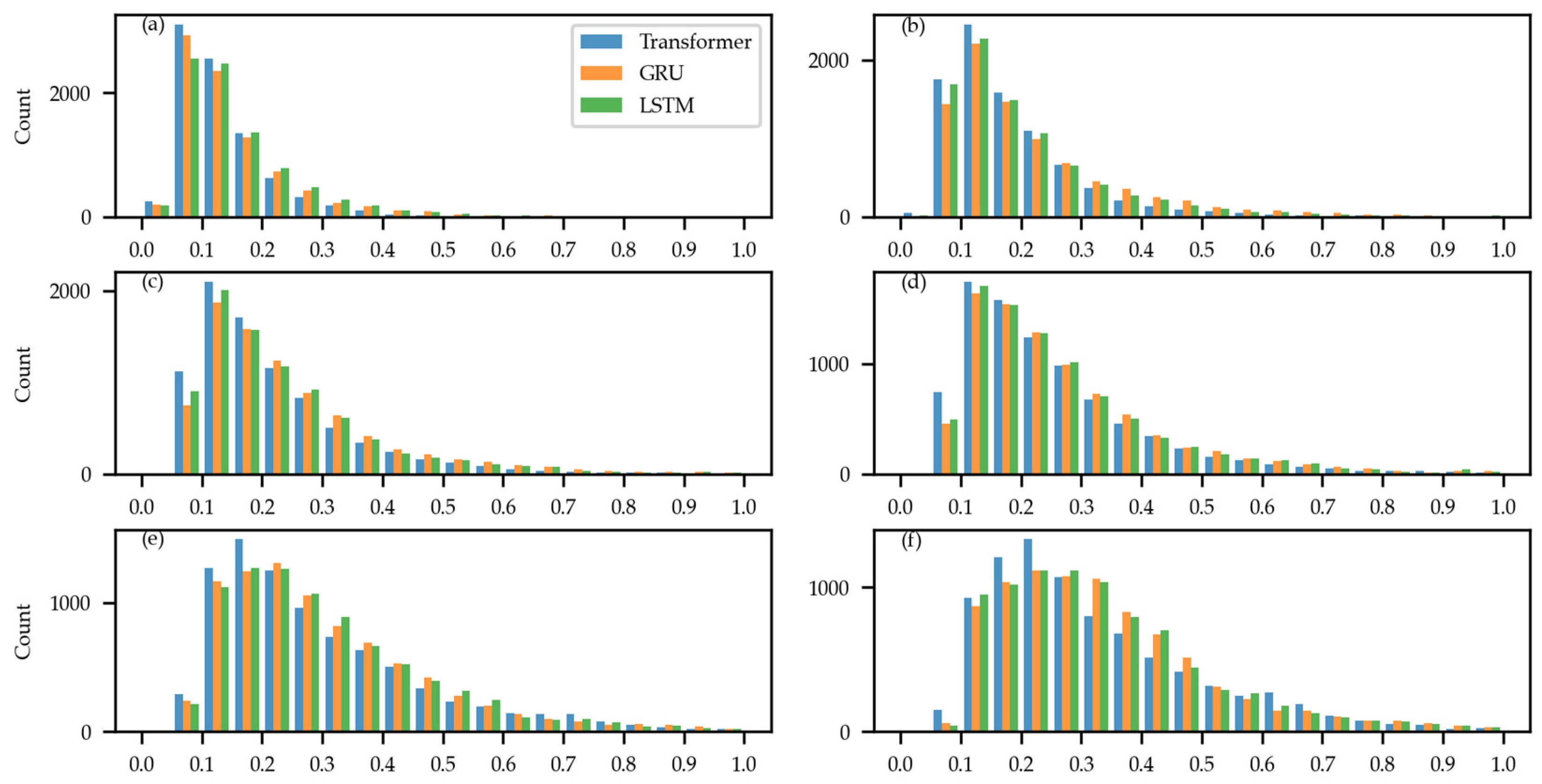
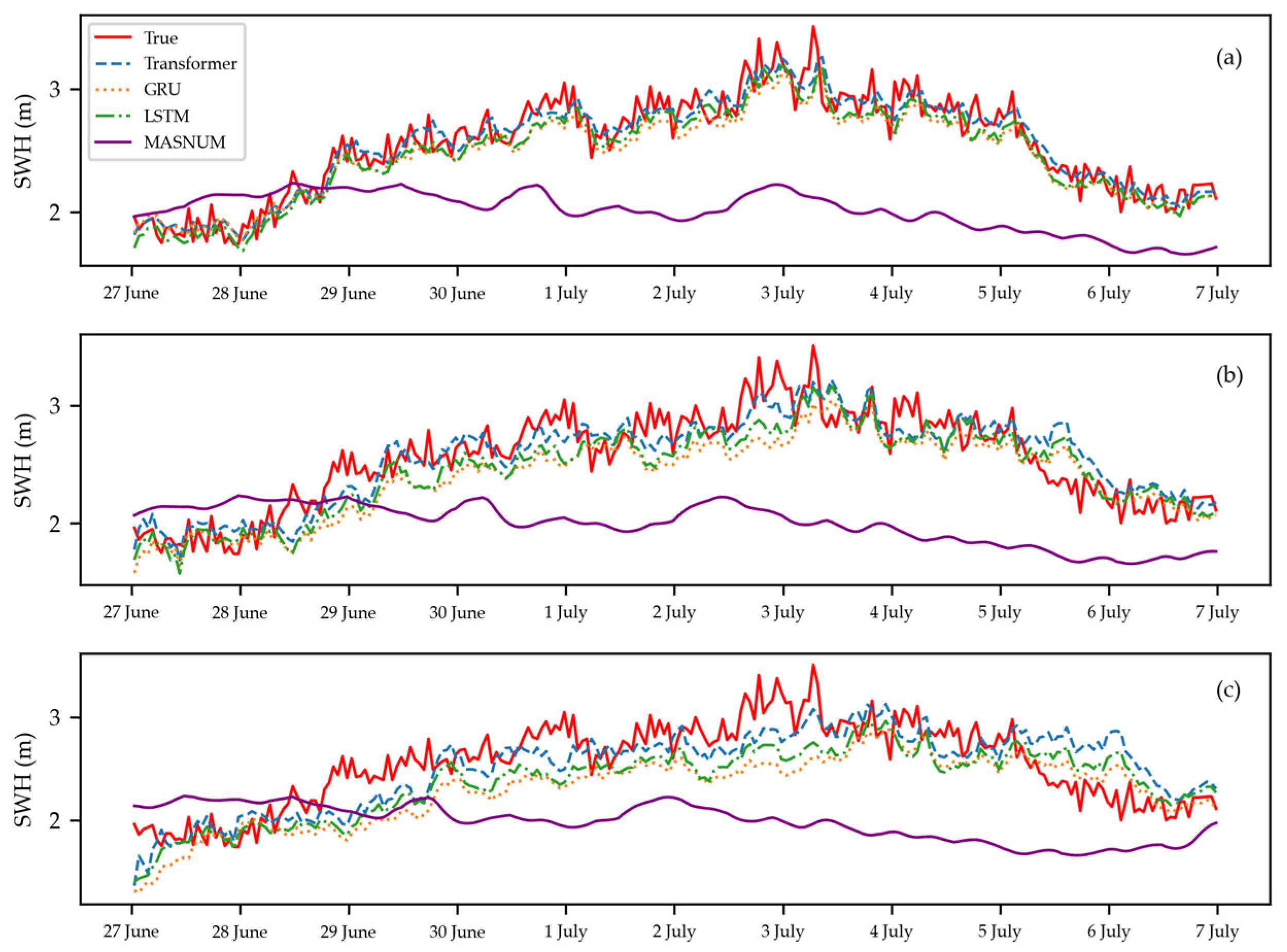
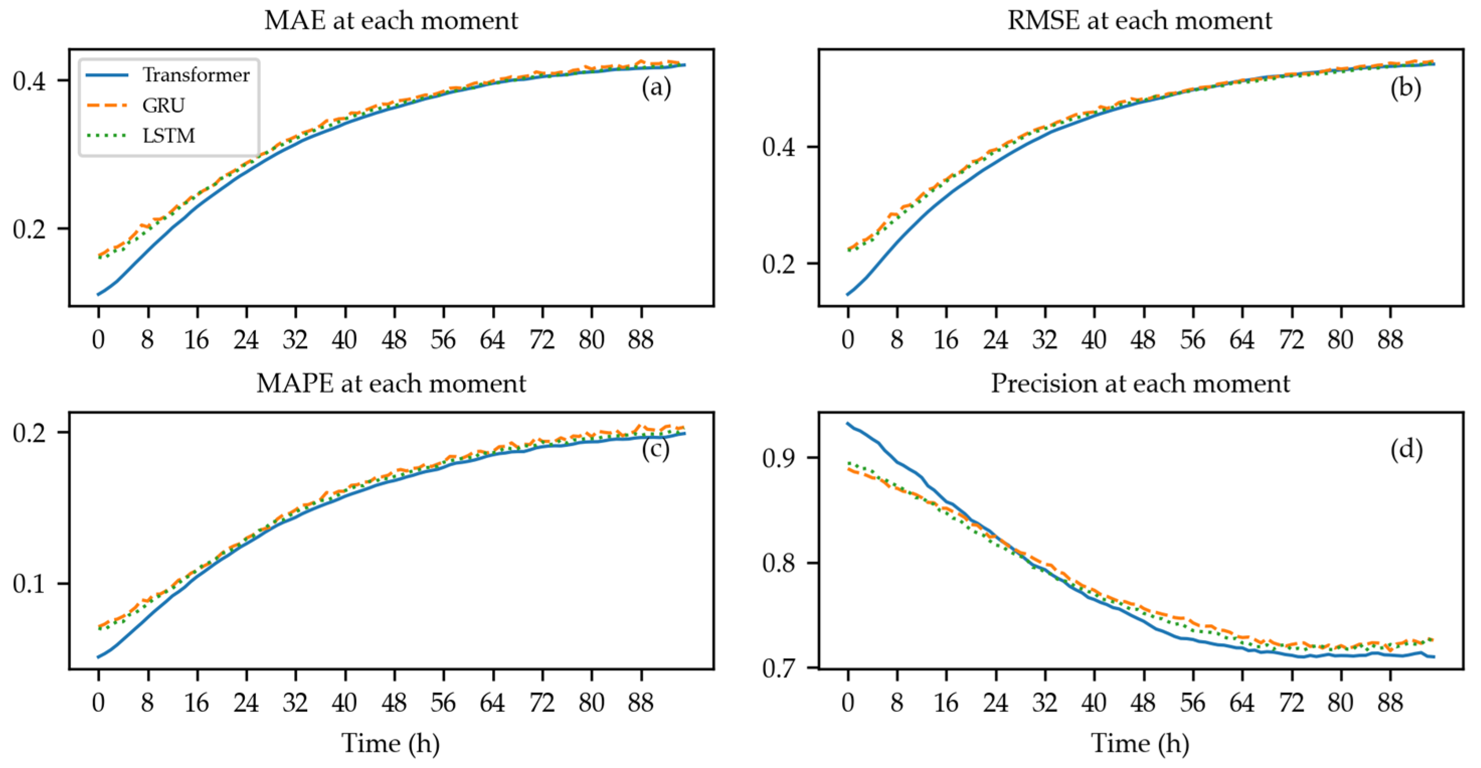
4. Results and Discussion

To explore the influence of different input sequence lengths on the forecasting results of sequences of the same length, Figure 6 shows the MAE results for the three machine-learning models, each using historical features from the previous 12 h, 24 h, 36 h, 48 h, 72 h, and 96 h as inputs, respectively, to forecast the SWHs of the next continuous 12 h. It can be seen that the transformer model results were less affected by different input sequence lengths, the error curve changed relatively smoothly, and the error results for different inputs were similar. However, the GRU and LSTM models showed variations in the forecasting performance under different input lengths. Our transformer model learned the dependencies between different positions in the input sequence through its attention mechanism. Thus, it was less affected by the length of the input sequence.
Table 5 presents the results of the multipoint average errors between the continuous 12 h, 24 h, 36 h, 48 h, 72 h, and 96 h forecasted SWHs and their corresponding true values. The machine-learning models outperformed the MASNUM numerical model in terms of MAE, RMSE, and MAPE within a 72 h time range. Interestingly, the MAE of the MASNUM numerical model was comparable to that of the LSTM model for predicting 96 consecutive hours. The error results of the MASNUM numerical model exhibited consistency across different prediction lengths, with the MAE ranging from 0.32 m to 0.34 m for consecutive 12–96 h and higher accuracy in wave scale classification for continuous 72–96 h. For the continuous forecasting, the transformer model performed similarly to the LSTM and GRU models. The MAE, RMSE, and MAPE between the true values and the forecasted values all showed a gradually increasing trend with increasing forecasting time. The accuracy of wave scale classification decreased gradually as the forecasting time increased. Overall, the transformer model outperformed the other two machine-learning models in terms of the average error results. For the continuous 12 h forecasting, our transformer model achieved an average MAE of 0.1394 m, an improvement of 8.4%, 14%, and 57% over GRU, LSTM, and the MASNUM numerical model, respectively, and had an average MAPE of 6.36%, an average bias of −0.0035, and a wave scale classification accuracy of 91%. In the case of continuous 96 h forecasting, our transformer model achieved an average MAE of 0.329 m, an improvement of 3.2%, 2.1%, and 2.2% over GRU, LSTM, and the MASNUM numerical model, respectively, and had an average MAPE of 15.29%, an average bias of 0.0004, and a wave scale classification accuracy of 77.47%. Therefore, the transformer model demonstrated superior accuracy in short-term wave scale classification warnings compared to the accuracies of the GRU, LSTM, and MASNUM numerical models.
Figure 7a–f present the frequency histograms of the average MAEs for continuous 12 h, 24 h, 36 h, 48 h, 72 h, and 96 h sequence forecasting. The transformer model exhibited a high frequency of small errors and a low frequency of large errors in terms of the MAEs compared to those of GRU and LSTM in the forecasting of different sequences, especially long sequences, as shown in Figure 7e,f.
To study the performance of the three models in continuous long-sequence forecasting, Figure 8a–c present the MAE, RMSE, and MAPE results at each time step during the continuous 96 h forecasting experiment. The MAEs, RMSEs, and MAPEs of the three models showed an increasing trend with the forecast time, but the error growth rate slowed. The fast accumulation of errors in the short term was related to the nonstationary fluctuations in the data. In the long-term forecasting, the models could capture the envolution and long-term dependencies in SWHs within a certain time range, resulting in a relatively slow error growth rate. Furthermore, the transformer model noticeably outperformed GRU and LSTM in the short term, while in the last 48 time steps, the MAEs, RMSEs, and MAPEs of all three models were very close to each other. Figure 8d shows the accuracy of continuous 96 h wave forecasting. Within the first 24 h, the transformer model exhibited higher accuracies in terms of wave scale classification than those of GRU and LSTM. However, beyond 24 h, the performance of our transformer method deteriorated compared to that of GRU and LSTM, indicating that the transformer model tended to overestimate the maximum values and underestimate the minimum values at the “wave scale level boundaries” more frequently than GRU and LSTM.
Typhoon Aere originated from a tropical disturbance in the east–southeast of Palau on 27 June 2022. It traveled northward, crossing the East China Sea, and made landfall on the northern island of Hokkaido, Japan, gradually dissipating thereafter. Figure 9 shows the three machine-learning models and MASNUM numerical model fitting results of wave height changes near the Hawaiian Islands within ten days of 27 June 2022. Figure 9a–c represent the forecasting results made 1 h, 12 h, and 24 h in advance, respectively. During this time period, there were large waves due to the influence of cyclones in the northwest Pacific, and the central Pacific waves responded to the strong atmospheric disturbances, leading to an increasing trend in SWH. All three machine-learning models accurately fit the SWH envolution within the 1 h forecast horizon, but underestimation was observed at the peak values, and overestimation was noted at the troughs. As the forecast horizon extended to 24 h, the accuracy of all three machine-learning models declined, but they still outperformed the MASNUM numerical models. The three machine-learning models consistently underestimated the SWH during the rising phase and overestimated them during the falling phase. The forecasting results of the transformer model were closer to the true values than those of GRU and LSTM. It is noteworthy that the three machine-learning models underestimated the prediction of SWH. This discrepancy can be attributed to the machine-learning models being trained on data primarily from normal conditions, with limited inclusion of typhoon-induced wave data. Consequently, the models may fail to accurately capture all the characteristics of wave envolution in the central and eastern Pacific Ocean during typhoons in the western Pacific. As a result, the forecast of SWH specifically related to typhoon-induced conditions may be flawed. To improve the prediction accuracy under extreme conditions, it is advisable to incorporate targeted training using typhoon-induced wave data, which may yield better outcomes [9].
According to the wave scale classification criteria, the waves near the Hawaiian Islands were mainly classified as moderate sea and rough sea. The evaluation results of various wave scale classifications forecasted using different sequences are shown in Table 6. In each sequence forecasting experiment, the classification results for moderate sea and rough sea were better, and the classification accuracies of these waves gradually decreased as the forecasting time increased. The classification accuracy of slight sea showed a trend of first decreasing and then increasing, while the classification accuracy of very rough sea showed a trend of first increasing and then decreasing.
Figure 10 shows the MAPE results for different wave scale levels. The MAPE for each wave scale level increased with the forecasting time, exhibiting an upward trend and depending on the data volume. The MAPE growth rate was slow for moderate sea and rough sea and the fastest for slight sea. Considering the accidental errors caused by the uneven sample distribution, the reliability of the transformer model in forecasting SWH for different wave scale levels was affected to some extent.
In summary, the transformer model, as with GRU and LSTM, could effectively forecast SWH with higher accuracies than the MANSNUM numerical model for continuous 72 h. However, during continuous forecasting, the transformer model’s generalizability was slightly better than that of the GRU and LSTM models. For long-sequence forecasting, the transformer model could focus on key time steps and important features, resulting in a better performance in short-term forecasting. Regarding the scale classification and warning of wave scale levels based on the forecasted results, the transformer model performed better in terms of short-term scale classification and warnings, achieving higher accuracy in warnings for moderate sea and rough sea, but performing poorly for slight sea and very rough sea.

5. Conclusions

Based on North Pacific Ocean buoy data, this study proposed the use of a transformer model to achieve continuous SWH forecasting using buoy wind field features, wave features, and environmental features. The transformer model weighted different parts of the input sequence, which helped the model to better identify important information and, thus, better capture the relationships between data. This research showed the following:
  • The transformer model extracted key information from wave data, realizing the continuous forecasting of waves and early warning of wave scale levels, with higher forecasting accuracies than those of the MASNUM numerical model and GRU and LSTM.
  • Unlike the GRU and LSTM models, our transformer method was less affected by the time length of the input sequence.
  • In the long-sequence forecasting process, the transformer model significantly outperformed the GRU and LSTM models in accurately forecasting future short-term wave height.
  • The wave scale levels in the sea area where the buoy was located were mainly moderate sea and rough sea, and the transformer model performed better in SWH forecasting and scale classification for these.
The transformer model considered both accuracy and continuity for forecasting, providing a reliable reference for continuous SWH forecasting and the early warning and forecasting of wave scale levels. The transformer model showed an advantage in the overall accuracy of long-sequence forecasting compared with that of the GRU and LSTM models, while it performed similarly to the other two models in terms of long-term wave scale classification and warnings. Due to training sample imbalance, there was a lack of reliability in classifying wave scale levels with a small number of samples. To address this issue, it is necessary to add “negative samples” to improve the model’s ability to fit negative samples.
The main difficulties in wave forecasting are the random nature and nonstationarity of wave data. The key to long-term sequence forecasting lies in the accuracy of long-term trend fitting. Therefore, the next phase of research will focus on handling the nonstationarity of wave data and improving the long-sequence forecasting ability of the transformer model. Data decomposition methods can be used to deconstruct nonstationary time series data into low-, medium-, and high-frequency signals, as well as trend, seasonal, and noise components, thus helping the model to fit different components of the data more accurately. The combination of these methods with the transformer model may allow the dependencies between data from multiple perspectives to be captured, providing research references for more accurate sequence forecasting.

Author Contributions

Conceptualization, T.S.; Data Curation, J.S.; Formal Analysis, J.S.; Funding Acquisition, T.S.; Investigation, J.S.; Methodology, J.S., T.S. and X.L.; Project Administration, J.S.; Resources, J.S., T.S. and F.W.; Software, J.S.; Supervision, T.S. and X.L.; Validation, J.S.; Visualization, J.S. and J.W.; Writing—Original Draft, J.S., T.S., X.L., J.C., Z.L. and J.C.; Writing—Review and Editing, J.S., T.S. and X.L. All authors have read and agreed to the published version of the manuscript.

Funding

This study was funded by the National Key Research and Development Program of China (Grant No. 2021YFC3101100), the Laoshan Laboratory (LSKJ202203003), and the National Natural Science Foundation of China (42149102).

Institutional Review Board Statement

Not applicable.

Informed Consent Statement

Not applicable.

Data Availability Statement

Buoy data used in this study are available from the National Data Buoy Center at https://www.ndbc.noaa.gov/ (accessed on 15 May 2023). GFS data used in this study are available from National Centers for Environmental Prediction at https://www.nco.ncep.noaa.gov/pmb/products/gfs/ (accessed on 20 August 2023).

Acknowledgments

The authors would like to thank the National Data Buoy Center and National Centers for Environmental Prediction for providing publicly accessible datasets.

Conflicts of Interest

The authors declare no conflict of interest.

References

  1. Dong, C.; Xu, G.; Han, G.; Bethel, B.J.; Xie, W.; Zhou, S. Recent Developments in Artificial Intelligence in Oceanography. Ocean. Land Atmos. Res. 2022, 2022, 9870950. [Google Scholar] [CrossRef]
  2. Zhang, X.; Han, Z.; Guo, X. Research progress in the application of deep learning to ocean information detection: Status and prospect. Mar. Sci. 2022, 46, 145–155. [Google Scholar]
  3. Prahlada, R.; Deka, P.C. Forecasting of Time Series Significant Wave Height Using Wavelet Decomposed Neural Network. In Proceedings of the International Conference on Water Resources, Coastal and Ocean Engineering (ICWRCOE), Mangaluru, India, 11–14 March 2015; pp. 540–547. [Google Scholar]
  4. Xia, T.; Li, X.; Yang, S. Prediction of wave height based on BAS-BP model in the northern part of the South China Sea. Trans. Oceanol. Limnol. 2021, 9–16. [Google Scholar]
  5. Jin, Q.; Hua, F.; Yang, Y. Prediction of the Significant Wave Height Based on the Support Vector Machine. Adv. Mar. Sci. 2019, 37, 199–209. [Google Scholar]
  6. Wang, Y.; Zhong, J.; Zhang, Z. Application of support vector regression in significant wave height forecasting. Mar. Forecast 2020, 37, 29–34. [Google Scholar]
  7. Berbic, J.; Ocvirk, E.; Carevic, D.; Loncar, G. Application of neural networks and support vector machine for significant wave height prediction. Oceanologia 2017, 59, 331–349. [Google Scholar] [CrossRef]
  8. Zhou, S.; Bethel, B.J.; Sun, W.; Zhao, Y.; Xie, W.; Dong, C. Improving Significant Wave Height Forecasts Using a Joint Empirical Mode Decomposition-Long Short-Term Memory Network. J. Mar. Sci. Eng. 2021, 9, 744. [Google Scholar] [CrossRef]
  9. Zhou, S.; Xie, W.; Lu, Y.; Wang, Y.; Zhou, Y.; Hui, N.; Dong, C. ConvLSTM-Based Wave Forecasts in the South and East China Seas. Front. Mar. Sci. 2021, 8, 680079. [Google Scholar] [CrossRef]
  10. Fan, S.; Xiao, N.; Dong, S. A novel model to predict significant wave height based on long short-term memory network. Ocean Eng. 2020, 205, 107298. [Google Scholar] [CrossRef]
  11. Jörges, C.; Berkenbrink, C.; Stumpe, B. Prediction and reconstruction of ocean wave heights based on bathymetric data using LSTM neural networks. Ocean Eng. 2021, 232, 109046. [Google Scholar] [CrossRef]
  12. Zhang, X.; Li, Y.; Gao, S.; Ren, P. Ocean Wave Height Series Prediction with Numerical Long Short-Term Memory. J. Mar. Sci. Eng. 2021, 9, 514. [Google Scholar] [CrossRef]
  13. Ma, J.; Xue, H.; Zeng, Y.; Zhang, Z.; Wang, Q. Significant wave height forecasting using WRF-CLSF model in Taiwan strait. Eng. Appl. Comput. Fluid Mech. 2021, 15, 1400–1419. [Google Scholar] [CrossRef]
  14. Feng, Z.; Hu, P.; Li, S.; Mo, D. Prediction of Significant Wave Height in Offshore China Based on the Machine Learning Method. J. Mar. Sci. Eng. 2022, 10, 836. [Google Scholar] [CrossRef]
  15. Xie, C.; Liu, X.; Man, T.; Xie, T.; Dong, J.; Ma, X.; Zhao, Y.; Dong, G. PWPNet: A Deep Learning Framework for Real-Time Prediction of Significant Wave Height Distribution in a Port. J. Mar. Sci. Eng. 2022, 10, 1375. [Google Scholar] [CrossRef]
  16. Meng, F.; Xu, D.; Song, T. ATDNNS: An adaptive time–frequency decomposition neural network-based system for tropical cyclone wave height real-time forecasting. Future Gener. Comput. Syst. 2022, 133, 297–306. [Google Scholar] [CrossRef]
  17. Alqushaibi, A.; Abdulkadir, S.J.; Rais, H.M.; Al-Tashi, Q.; Ragab, M.G.; Alhussian, H. Enhanced Weight-Optimized Recurrent Neural Networks Based on Sine Cosine Algorithm for Wave Height Prediction. J. Mar. Sci. Eng. 2021, 9, 524. [Google Scholar] [CrossRef]
  18. Hao, P.; Li, S.; Yu, C.; Wu, G. A Prediction Model of Significant Wave Height in the South China Sea Based on Attention Mechanism. Front. Mar. Sci. 2022, 9, 895212. [Google Scholar] [CrossRef]
  19. Wang, L.; Deng, X.; Ge, P.; Dong, C.; Bethel, B.J.; Yang, L.; Xia, J. CNN-BiLSTM-Attention Model in Forecasting Wave Height over South-East China Seas. Comput. Mater. Contin. 2022, 73, 2151–2168. [Google Scholar] [CrossRef]
  20. Luo, Q.; Xu, H.; Bai, L. Prediction of significant wave height in hurricane area of the Atlantic Ocean using the Bi-LSTM with attention model. Ocean Eng. 2022, 266, 112747. [Google Scholar] [CrossRef]
  21. Li, X.; Cao, J.; Guo, J.; Liu, C.; Wang, W.; Jia, Z.; Su, T. Multi-step forecasting of ocean wave height using gate recurrent unit networks with multivariate time series. Ocean Eng. 2022, 248, 110689. [Google Scholar] [CrossRef]
  22. Wang, J.; Wang, Y.; Yang, J. Forecasting of Significant Wave Height Based on Gated Recurrent Unit Network in the Taiwan Strait and Its Adjacent Waters. Water 2021, 13, 86. [Google Scholar] [CrossRef]
  23. Yevnin, Y.; Chorev, S.; Dukan, I.; Toledo, Y. Short-term wave forecasts using gated recurrent unit model. Ocean Eng. 2022, 268, 113389. [Google Scholar] [CrossRef]
  24. Meng, F.; Song, T.; Xu, D.; Xie, P.; Li, Y. Forecasting tropical cyclones wave height using bidirectional gated recurrent unit. Ocean Eng. 2021, 234, 108795. [Google Scholar] [CrossRef]
  25. Sukanda, A.J.T.; Adytia, D. Wave Forecast using Bidirectional GRU and GRU Method Case Study in Pangandaran, Indonesia. In Proceedings of the 2022 International Conference on Data Science and Its Applications (ICODSA), Bandung, Indonesia, 6–7 July 2022; pp. 278–282. [Google Scholar]
  26. Celik, A. Improving prediction performance of significant wave height via hybrid SVD-Fuzzy model. Ocean Eng. 2022, 266, 113173. [Google Scholar] [CrossRef]
  27. Vaswani, A.; Shazeer, N.; Parmar, N.; Uszkoreit, J.; Jones, L.; Gomez, A.N.; Kaiser, L.; Polosukhin, I. Attention Is All You Need. In Advances in Neural Information Processing Systems, Proceedings of the 31st Conference on Neural Information Processing Systems, Long Beach, CA, USA, 4–9 December 2017; Curran Associates Inc.: Red Hook, NY, USA, 2017; Volume 30. [Google Scholar]
  28. Dong, L.; Xu, S.; Xu, B. Speech-Transformer: A No-Recurrence Sequence-to-Sequence Model for Speech Recognition. In Proceedings of the 2018 IEEE International Conference on Acoustics, Speech and Signal Processing (ICASSP), Calgary, AB, Canada, 15–20 April 2018; pp. 5884–5888. [Google Scholar]
  29. Dosovitskiy, A.; Beyer, L.; Kolesnikov, A.; Weissenborn, D.; Zhai, X.; Unterthiner, T.; Dehghani, M.; Minderer, M.; Heigold, G.; Gelly, S.; et al. An image is worth 16x16 words: Transformers for image recognition at scale. arXiv 2021, arXiv:2010.11929. [Google Scholar] [CrossRef]
  30. Zhou, H.; Zhang, S.; Peng, J.; Zhang, S.; Li, J.; Xiong, H.; Zhang, W. Informer: Beyond Efficient Transformer for Long Sequence Time-Series Forecasting. In AAAI Conference on Artificial Intelligence, Proceedings of the 35th AAAI Conference on Artificial Intelligence 33rd Conference on Innovative Applications of Artificial Intelligence 11th Symposium on Educational Advances in Artificial Intelligence, Washington, DC, USA, 2–9 February 2021; AAAI Press: Washington, DC, USA, 2021; Volume 35, pp. 11106–11115. [Google Scholar]
  31. Wu, H.; Xu, J.; Wang, J.; Long, M. Autoformer: Decomposition Transformers with Auto-Correlation for Long-Term Series Forecasting. In Advances in Neural Information Processing Systems, Proceedings of the 35th Conference on Neural Information Processing Systems (NeurIPS 2021), Electr Network, 6–14 December 2021; NeurIPS Proceedings: San Diego, CA, USA, 2021; Volume 34. [Google Scholar]
  32. Tuli, S.; Casale, G.; Jennings, N.R. TranAD: Deep Transformer Networks for Anomaly Detection in Multivariate Time Series Data. Proc. Vldb. Endow. 2022, 15, 1201–1214. [Google Scholar] [CrossRef]
  33. Zerveas, G.; Jayaraman, S.; Patel, D.; Bhamidipaty, A.; Eickhoff, C. A Transformer-based Framework for Multivariate Time Series Representation Learning. In Proceedings of the 27th ACM SIGKDD International Conference on Knowledge Discovery and Data Mining (KDD), Electr Network, 14–18 August 2021; AAAI Press: Washington, DC, USA, 2021; pp. 2114–2124. [Google Scholar]
  34. Wen, Q.; Zhou, T.; Zhang, C.; Chen, W.; Ma, Z.; Yan, J.; Sun, L. Transformers in Time Series: A Survey. arXiv 2022, arXiv:2202.07125. [Google Scholar]
  35. Immas, A.; Do, N.; Alam, M.R. Real-time in situ prediction of ocean currents. Ocean Eng. 2021, 228, 108922. [Google Scholar] [CrossRef]
  36. Zhou, L.; Zhang, R. A self-attention-based neural network for three-dimensional multivariate modeling and its skillful ENSO predictions. Sci. Adv. 2023, 9, eadf2827. [Google Scholar] [CrossRef]
  37. Ye, F.; Hu, J.; Huang, T.; You, L.; Weng, B.; Gao, J. Transformer for EI Niño-Southern Oscillation Prediction. IEEE Geosci. Remote Sens. Lett. 2022, 19, 1003305. [Google Scholar] [CrossRef]
  38. Pokhrel, P.; Ioup, E.; Simeonov, J.; Hoque, M.T.; Abdelguerfi, M. A Transformer-Based Regression Scheme for Forecasting Significant Wave Heights in Oceans. IEEE J. Ocean Eng. 2022, 47, 1010–1023. [Google Scholar] [CrossRef]
  39. Chang, W.; Li, X.; Dong, H.; Wang, C.; Zhao, Z.; Wang, Y. Real-Time Prediction of Ocean Observation Data Based on Transformer Model. In Proceedings of the 2021 ACM International Conference on Intelligent Computing and its Emerging Applications, Jinan, China, 28–29 December 2021; Association for Computing Machinery: New York, NY, USA, 2021; pp. 83–88. [Google Scholar]
  40. Ham, Y.G.; Kim, J.H.; Luo, J. Deep learning for multi-year ENSO forecasts. Nature 2019, 573, 568–572. [Google Scholar] [CrossRef] [PubMed]
  41. Putri, D.A.; Adytia, D. Time Series Wave Forecasting with Transformer Model, Case Study in Pelabuhan Ratu, Indonesia. In Proceedings of the 2022 10th International Conference on Information and Communication Technology (ICoICT), Bandung, Indonesia, 2–3 August 2022; pp. 430–434. [Google Scholar]
  42. Li, J.; Zhou, L.; Zheng, C.; Han, X.; Chen, X. Spatial-temporal variation analysis of sea wave field in the Pacific Ocean. Mar. Sci. 2012, 36, 94–100. [Google Scholar]
  43. Liu, J.; Jiang, W.; Yu, M.; Ni, J.; Liang, G. An analysis on annual variation of monthly mean sea wave fields in north Pacific Ocean. J. Trop. Oceanogr. 2002, 21, 64–69. [Google Scholar]
  44. Allahdadi, M.N.; Ruoying, H.R.; Neary, V.S. Predicting ocean waves along the US east coast during energetic winter storms: Sensitivity to whitecapping parameterizations. Ocean Sci. 2019, 15, 691–715. [Google Scholar] [CrossRef]
  45. GB/T 12763.2-2007; Specifications for Oceanographic Survey—Part 2: Marine Hydrographic Observation. Inspection and Quarantine of the People’s Republic of China and Standardization Administration of China: Qingdao, China, 2007.
  46. Srivastava, N.; Hinton, G.; Krizhevsky, A.; Sutskever, I.; Salakhutdinov, R. Dropout: A Simple Way to Prevent Neural Networks from Overfitting. J. Mach. Learn Res. 2014, 15, 1929–1958. [Google Scholar]
  47. Kingma, D.P.; Ba, J. Adam: A Method for Stochastic Optimization. arXiv 2015, arXiv:1412.6980. [Google Scholar] [CrossRef]
  48. Cho, K.; van Merrienboer, B.; Gulcehre, C.; Bahdanau, D.; Bougares, F.; Schwenk, H.; Bengio, Y. Learning Phrase Representations using RNN Encoder-Decoder for Statistical Machine Translation. arXiv 2014, arXiv:1406.1078. [Google Scholar]
  49. Hochreiter, S.; Schmidhuber, J. Long Short-Term Memory. Neural Comput. 1997, 9, 1735–1780. [Google Scholar] [CrossRef]
  50. Yang, Y.; Qiao, F.; Zhao, W.; Teng, Y.; Yuan, L. MASNUM ocean wave numerical model in spherical coordinates and its application. Acta Oceanol. Sin. 2005, 27, 1–2. [Google Scholar]
Figure 1. Geographical location of the buoy.
Jmse 11 01821 g001
Figure 2. Wind rose and wave rose.
Jmse 11 01821 g002
Figure 3. Correlation matrix between features.
Jmse 11 01821 g003
Figure 4. The transformer network structure [27]. N is the numer of Encoder stacks and M is the numer of Decoder stacks.
Jmse 11 01821 g004
Figure 5. Correspondence between input and output sequences.
Jmse 11 01821 g005
Figure 6. Comparison of MAE results for continuous 12 h output forecasting corresponding to 12, 24, 36, 48, 72, and 96 h input sequence lengths between transformer (blue), GRU (orange), and LSTM (green).
Jmse 11 01821 g006
Figure 7. Comparison of frequency histograms of the average MAE distribution between transformer (blue), GRU (orange), and LSTM (green) at (a) 12, (b) 24, (c) 36, (d) 48, (e) 72, and (f) 96 h time lengths.
Jmse 11 01821 g007
Figure 8. Comparison of (a) MAE; (b) RMSE; (c) MAPE; (d) Precision at different time steps of continuous 96 h forecasting results from transformer (blue), GRU (orange), and LSTM (green).
Jmse 11 01821 g008
Figure 9. Comparison of wave height changes within a ten-day period of 27 June 2022 between real values (red) and SWH forecasting results from transformer (blue), GRU (orange), LSTM (green), and MASNUM (purple) at the (a) 1, (b) 12, (c) 24 h windows.
Jmse 11 01821 g009
Figure 10. Average MAPE results from transformer forecasting for slight sea (blue), moderate sea (orange), rough sea (green), and very rough sea (red) at continuous 12, 24, 36, 48, 72, and 96 h forecasting.
Jmse 11 01821 g010
Table 1. Detailed buoy information.
Location17°2′32″ N, 157°44′47″ W
Site elevationsea level
Air temp height3.7 m above site elevation
Anemometer height4.1 m above site elevation
Barometer elevation2.7 m above mean sea level
Sea temp depth1.5 m below water line
Water depth4997 m
Watch circle radius4691.7864 m
Table 2. Detailed SWH information.
Station IdMax_SWHMin_SWHMean_SWHVariance_SWH
510025.92 m0.49 m2.33 m0.36
Table 3. Valid sample time range and quantity information.
DatasetTime_RangeValid Sample Numbers
Training set1 January 2000–31 December 2018117,706
Validation set1 October 2019–31 December 202118,716
Test set1 January 2022–31 December 20228760
Table 4. The optimal combinations of encoder/decoder stacks.
Forecast HoursEncoder Stacks (N)Decoder Stacks (M)
1211
2411
3621
4861
7222
9642
Table 5. Comparison of the average errors for continuous 12, 24, 36, 48, 72, and 96 h forecasting between transformer, GRU, and LSTM. The bold text in the table represents the optimal forecast value.
Forecast HoursModelBiasMAERMSEMAPEPrecision
12 hTransformer−0.00350.13940.19396.36%91.09%
GRU0.06560.15220.21926.72%90.31%
LSTM0.07130.16210.22657.18%89.58%
MASNUM0.01480.32390.407715.12%81.16%
24 hTransformer−0.01460.18640.26138.57%88.38%
GRU0.11410.22560.32039.82%85.53%
LSTM0.08300.20540.29109.05%86.76%
MASNUM0.01530.32420.412115.16%81%
36 hTransformer0.02610.22300.314610.17%85.97%
GRU0.11000.25670.358011.32%83.51%
LSTM0.08590.24230.340710.75%84.26%
MASNUM0.01510.32420.423415.16%80.67%
48 hTransformer0.02360.25420.354711.67%83.3%
GRU0.06830.27760.384512.53%82.35%
LSTM0.07870.27080.376112.14%82.15%
MASNUM0.01630.32430.435115.2%80.5%
72 hTransformer0.01860.30200.414513.93%78.9%
GRU0.0410.31100.423614.28579.62%
LSTM0.05780.31330.425614.29%78.79%
MASNUM0.01680.32750.455615.31%80.01%
96 hTransformer0.00040.32900.446515.29%77.47%
GRU0.02470.33980.455815.79%77.73%
LSTM0.02580.33620.452115.62%77.42%
MASNUM0.01720.33630.478315.45%79.75%
Table 6. Comparison of the mean precision results from transformer forecasting for various wave scale classifications at continuous 12, 24, 36, 48, 72, and 96 h forecasting.
Classification12 h_Mean24 h_Mean36 h_Mean48 h_Mean72 h_Mean96 h_Mean
Slight sea40%33%24%18%17%37%
Moderate sea94%92%89%88%84%82%
Rough sea83%77%76%69%61%57%
Very rough sea39%36%40%41%41%24%
Disclaimer/Publisher’s Note: The statements, opinions and data contained in all publications are solely those of the individual author(s) and contributor(s) and not of MDPI and/or the editor(s). MDPI and/or the editor(s) disclaim responsibility for any injury to people or property resulting from any ideas, methods, instructions or products referred to in the content.

