3D-EddyNet: A Novel Approach for Identifying Three-Dimensional Morphological Features of Mesoscale Eddies in the Ocean

Abstract

Mesoscale eddies are characterized by swirling currents spanning from tens to hundreds of kilometers in diameter three-dimensional attributes holds paramount significance in driving advancements in both oceanographic research and engineering applications. Nonetheless, a notable absence of models capable of adeptly harnessing the scarcity of high-quality annotated marine data, to efficiently discern the three-dimensional morphological attributes of mesoscale eddies, is evident. To address this limitation, this paper constructs an innovative deep-learning-based model termed 3D-EddyNet, tailored for the precise identification and visualization of mesoscale eddies. In contrast to the prevailing 2D models that remain confined to surface-level data, 3D-EddyNet takes full advantage of three-dimensional convolutions to capture the essential characteristics of eddies. It is specifically tailored for recognizing spatial features within mesoscale eddies, including parameters like position, radius, and depth. The combination of dynamic convolutions and residual networks effectively enhances the model’s performance in a synergistic manner. The model employs the PReLU activation function to tackle gradient vanishing issues and improve convergence rates. It also addresses the challenge of foreground–background imbalance through cross-entropy functions. Additionally, to fine-tune the model’s effectiveness during the training phase, techniques such as random dropblock and batch normalization are skillfully incorporated. Furthermore, we created a training dataset using HYCOM data specifically from the South China Sea region. This dataset allowed for a comprehensive analysis of the spatial-temporal distribution and three-dimensional morphology of the eddies, serving as an assessment of the model’s practical effectiveness. The culmination of this analysis reveals an impressive 20% enhancement over 3D-UNet in detection accuracy, coupled with expedited convergence speed. Notably, the results obtained through our detection using empirical data align closely with those obtained by other scholars. The mesoscale eddies within this specific region unveil a discernible northeast-to-southwest distribution pattern, categorized into three principal morphological classifications: bowl-shaped, olive-shaped, and nearly cylindrical, with the bowl-shaped eddies prominently dominating.

1. Introduction

The ocean, covering 71% of the Earth’s surface, stands as one of the largest ecosystems. Ocean currents, as the primary form of seawater movement, play a crucial role in material and energy transfer and climate change.

Mesoscale eddies, widely active in the ocean, are essentially a distinct type of oceanic front, distributed throughout the world’s major oceans [1]. They exhibit a relatively closed circulation structure, with diameters ranging from tens to hundreds of kilometers. Based on their direction and the temperature anomalies at their cores, mesoscale eddies are commonly categorized as cold or warm eddies [2]. The first discovery of mesoscale eddies dates back to 1970 when Soviet ocean scientists conducted ocean current observation experiments in the northeast Atlantic. These eddies, with spatial scales of 100 km and temporal scales of several months, exhibited flow velocities of around 10 cm/s. Since then, scientists have been aware of the impact of mesoscale eddies on ocean circulation and marine ecosystems [3]. These eddies have extensive movement distances and a broad influence, significantly altering temperature and salinity distribution in the ocean and playing a crucial role in material exchange and distribution [4]. Furthermore, mesoscale eddies harbor substantial kinetic energy, accounting for over 80% to 90% of the total oceanic circulation energy [5]. To gain a deeper understanding of the characteristics and impact of mesoscale eddies on the ocean, marine scientists have conducted various explorations, and such efforts heavily rely on eddy identification. Traditionally, identification methods can be broadly categorized into Eulerian and Lagrangian approaches [6] depending on the type of dataset used. However, these conventional methods often require manual supervision and expert prior knowledge, making it challenging to simultaneously process and analyze diverse formats of mesoscale eddy observational data.

In recent years, with the rapid development and maturation of machine learning, and the widespread use of satellite observations, marine science has encountered new opportunities. As observational data related to mesoscale eddies continue to increase, identification methods have also evolved, with many scholars attempting deep-learning-based approaches to enhance mesoscale eddy identification and enrich observational capabilities. For instance, Lguensat et al. [7] developed EddyNet, a deep neural network for the pixel-level classification of oceanic eddies. Although several researchers further refined this method, including EddyNet_S and EddyResNet, the accuracy of this series of methods falls short compared to traditional detection methods. Other studies, like that of Xu et al. [8], employed a vector-geometry-based algorithm in conjunction with the PSPNet model for intelligent eddy detection. Nevertheless, the limitation of this algorithm lies in its insensitivity to the widely dominant asymmetrical eddy structures in the ocean [9]. Moschos et al. [10] introduced a novel method, DEEP-SST-EDDIES, which combines deep learning with Sea Surface Temperature (SST) data to detect eddy features. However, these methods often require substantial labeled datasets for training. To address this issue, Duo et al. [11] proposed OEDNet, a method for mesoscale eddy detection that employs data augmentation and target detection networks, mitigating the need for an abundance of annotated data. Each detection and identification method serves different scenarios and problems, providing systematic understanding and references for the advancement of mesoscale eddy detection and recognition research.

Early studies of mesoscale eddies primarily relied on altimetry data to conduct statistical analysis on surface information. However, the changes in oceanic physical parameters caused by mesoscale eddies are not solely evident on the sea surface but are also reflected in the subsurface layer. Oceanic three-dimensional temperature, salinity, and sound field structures reveal distinct mesoscale eddy characteristics [12]. Although accumulated altimetry data have provided considerable insights into mesoscale dynamics, they lack information regarding subsurface eddy structures, making it challenging to gain comprehensive knowledge of the three-dimensional morphology of mesoscale eddies. As discussed earlier, the methods mainly focused on the ocean surface, and the use of deep learning for the identification of mesoscale eddy three-dimensional structures remains an unexplored domain. In recent years, as marine observation platforms have been increasingly improved, and more observation methods have emerged, such as the Array for Real-time Geostrophic Oceanography (Argo) float system, Lagrangian drift floats, underwater gliders, satellite synthetic aperture radar, numerical simulations, temperature and salinity profiling instruments, and other advanced technologies [13], coupled with established satellite altimetry observation platforms, researchers now possess the ability to observe mesoscale eddies from the surface to the deep sea. This provides the necessary data foundation to investigate the overall structure of subsurface mesoscale eddies.

Studying eddies using model data is an essential approach. Dong et al. [6] conducted research based on high-resolution Regional Ocean Model System (ROMS) data, analyzing the three-dimensional temperature and salinity structures of eddies in the South China Sea and generating a large-scale mesoscale eddy three-dimensional dataset. Lin et al. [14] further analyzed the three-dimensional temperature and salinity structures of eddies, demonstrating that eddies in the South China Sea present three different forms: surface-enhanced, middle-layer-enhanced, and bottom-layer-enhanced. Yang et al. [15] similarly employed ROMS data to analyze nearly 50,000 mesoscale eddies detected from nineteen years of Northwest Tropical Pacific sea level height records. They further explored the three-dimensional eddy structures using a composite eddy flow chart. Zhang et al. [16] applied eddy detection and tracking algorithms based on the Oceanic General Circulation Model for the Earth Simulator (OFES) data, developed jointly by the Japan Agency for Marine-Earth Science and Technology (JAMSTEC) and the National Oceanic and Atmospheric Administration (NOAA). They synthesized identified cyclonic and anticyclonic eddies’ three-dimensional structures from the simulated horizontal velocity vector to obtain a comprehensive understanding of mesoscale eddies in the Northwest Pacific.

However, model data are inevitably subject to errors due to the integration of various ocean observation data, and as navigational capabilities improve and observational instruments continue to update, along with the abundance of Argo profiles, researchers can conduct more effective studies using observational data. Exploring the influence of mesoscale eddies on vertical temperature and salinity structures has greatly contributed to our understanding of their three-dimensional morphology. For example, Chaigneau et al. [17] combined six years of Argo profiles into eddies, resulting in the average vertical structure of eddies in the East and West Pacific. They found that the core depths of cyclonic and anticyclonic eddies differ (approximately 150 m and 400 m, respectively). He et al. [18] analyzed mesoscale eddy data in the South China Sea from 1993 to 2015, updating the statistical data of surface eddy characteristics in the South China Sea. By placing more than 7000 historical Argo profiles in the center coordinate system of eddies, they revealed the composite average three-dimensional structure of eddies. Prants et al. [19] traced eddy trajectories and important events during the eddy lifecycle, discussing and analyzing the vertical structure and hydrological characteristics derived from the shipborne and profile data of Argo floats.

With the rapid development of deep learning, researchers have recently begun applying it to underwater scenarios. Md. Moniruzzaman et al. [20] systematically described the application of deep learning in underwater image analysis, classifying analysis methods based on the objects being detected, and focusing on the deep learning architectures used. To handle three-dimensional data, Cicek et al. [21] extended the U-Net architecture to 3D data, creating the 3D-UNet network. Although initially applied to medical image segmentation, the similarity in data properties between 3D-UNet and mesoscale eddies presents an inspiring method for identifying their three-dimensional features. V-Net (Milletari et al. [22]) is another method that replaces 2D convolutions with 3D convolutions in U-Net and introduces short skip connections, optimizing the model’s performance to better suit three-dimensional data. Furthermore, Haoyu et al. [23] introduced a double attention mechanism to the 3D-UNet segmentation model, incorporating spatial attention modules and channel attention modules in both the upsampling and downsampling processes. This enables end-to-end training for 3D-UNet. In this paper, taking advantage of the continuous accumulation and updates of marine data and the ongoing progress in neural network models across various fields, we will employ deep learning methods to explore the three-dimensional structure of mesoscale eddies.

2. 3D-EddyNet Model or Methods

Ocean satellite remote sensing, such as sea surface height images and ocean model data, offers high spatial resolution, providing a solid data foundation for employing neural network methods. However, the complexity of mesoscale eddy data poses significant challenges for detecting algorithms. Ensuring that the trained deep learning model can effectively identify mesoscale eddies remains a challenge. While deep learning has achieved certain successes in mesoscale eddy identification and prediction, existing methods are limited to the ocean surface, failing to provide information on subsurface eddy structures and impeding progress in three-dimensional structure research.

Some scholars have initiated preliminary explorations of the three-dimensional structures of mesoscale eddies based on Argo observational data and ocean model data. However, these methods require human involvement and rely heavily on prior knowledge, making them difficult to generalize. Research on using deep learning for the three-dimensional morphological feature identification of mesoscale eddies is still in its infancy, offering vast potential for further exploration.

2.1. 3D Convolutional

To establish a network model for identifying the three-dimensional morphological features of mesoscale eddies, a necessary condition is to extract three-dimensional spatial information through convolutional layers.

The convolutional layer is a key operation in CNN, typically in the form of two-dimensional convolution, with the following calculation formula:

$$x_j^{l+1}=f({\sum }_{i\in M_j}{x}_i^l\times w_{ij}^{l+1}+b_j^{l+1})$$

(1)

In neural networks, neurons are organized into layers, where each neuron receives input from neurons in the previous layer and provides output to neurons in the next layer. $x_j^{l+1}$ represents the value of the jth neuron in layer l + 1, and $x_i^l$ represents the value of the ith neuron in layer l. The connection between the ith and jth neurons is represented by the weight $W_{\mathrm{ij}}^{l+1}$, and the output is influenced by the bias $b_j^{l+1}$. An activation function $f$ is applied to the weighted sum of inputs. 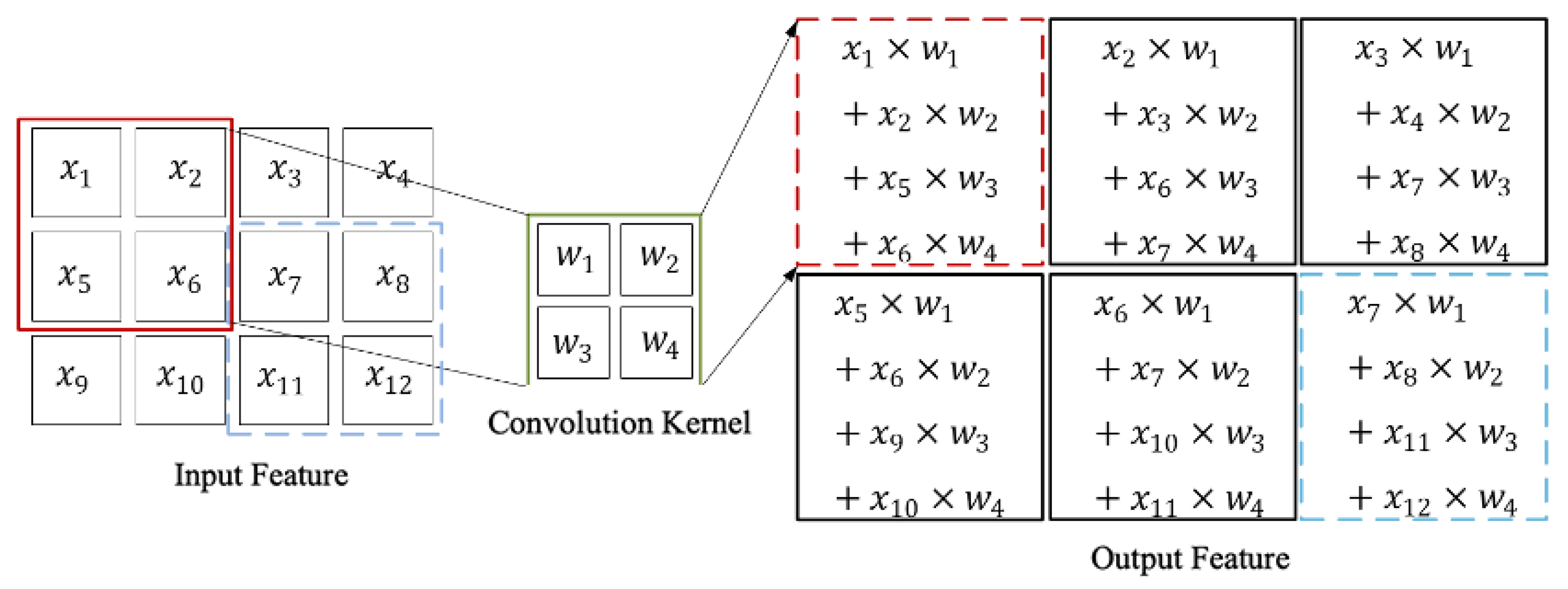Figure 1 illustrates the main steps of the convolutional operation. After obtaining the features through convolution, pooling operation aggregates local features in the image through statistical operations, further extracting features and improving the network’s computational efficiency.

In the current field of computer vision, there is an increasing demand for 3D data processing techniques. 3D convolution can extract voxel-related features in three-dimensional space, enabling the end-to-end mapping of 3D volume data, making it a crucial technique for processing 3D data. Compared to 2D convolution, 3D convolution can better capture spatial features along the depth dimension, thus having an advantage when dealing with data that require a consideration of temporal or spatial depth. For instance, 3D convolution is better suited for handling three-dimensional ocean images with spatial depth, exploring the spatial correlations in the data and addressing the limitation of 2D convolution in capturing vertical features.

The dimension of the convolutional kernel refers to the dimension in which the sliding window operation is performed, not involving the channel dimension. Regardless of the number of channels, they share the same sliding window position. Although the weights of the convolutional kernels on each channel are independent in 2D multi-channel convolution, the sliding window position is shared. Therefore, when discussing the dimension of the convolutional kernel, the number of channels is not taken into account.

For a single-channel input, with input size (1, height, width), and a kernel size of $(1,k_h,k_w)$, the convolutional kernel slides over the input image, performing the convolution operation between the sliding window and the values inside the kernel. In recent times, the correlation operation is commonly used instead of convolution, resulting in one value in the output image. The illustration in Figure 1 shows a 2D single-channel convolution with input data of size 3 × 4, a kernel size of 2 × 2, and a stride of 1.

In the context of multi-channel scenarios, when the input image has three channels, denoted as (3, height, width), and the kernel size is (3, $k_h$, $k_w$), the convolutional operation occurs in both dimensions (height and width) of the input. At each step, the kernel slides over the entire window of all channels in the input, performing the operation. Then, the information from all channels is aggregated to form a single output channel, resulting in the complete compression of multi-channel information.

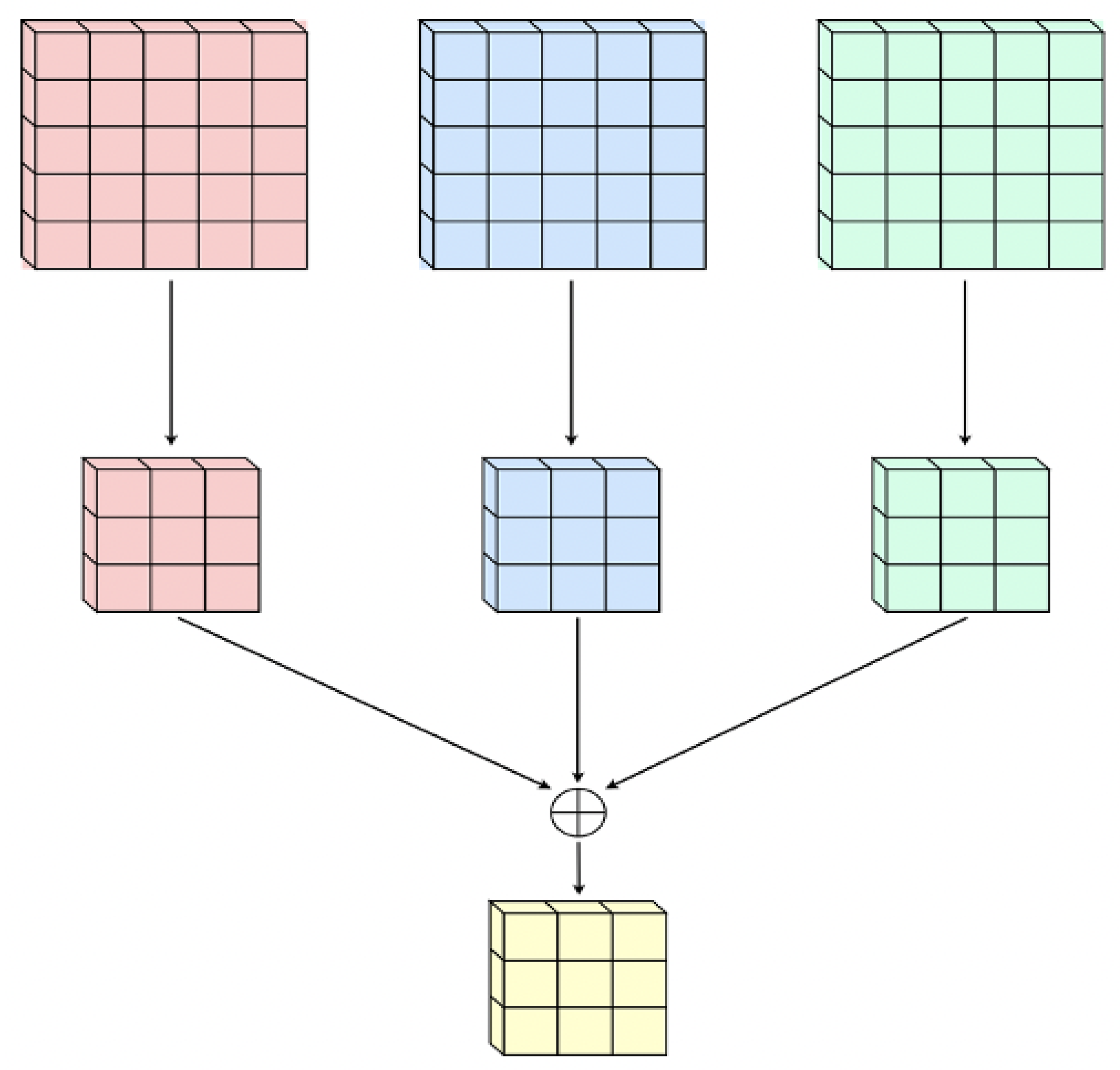
The process of 2D multi-channel convolution is as follows: each kernel is applied to the input channels of the previous layer to generate one output channel. This process is repeated for all kernels to generate multiple channels, as shown in Figure 2.

This process can be seen as sliding a 3D filter matrix over the input layer. The number of channels in the input layer is the same as the number of kernels in the filter. The 3D filter moves only in the height and width directions of the image. At each sliding position, element-wise multiplication and addition are performed, resulting in a single number.

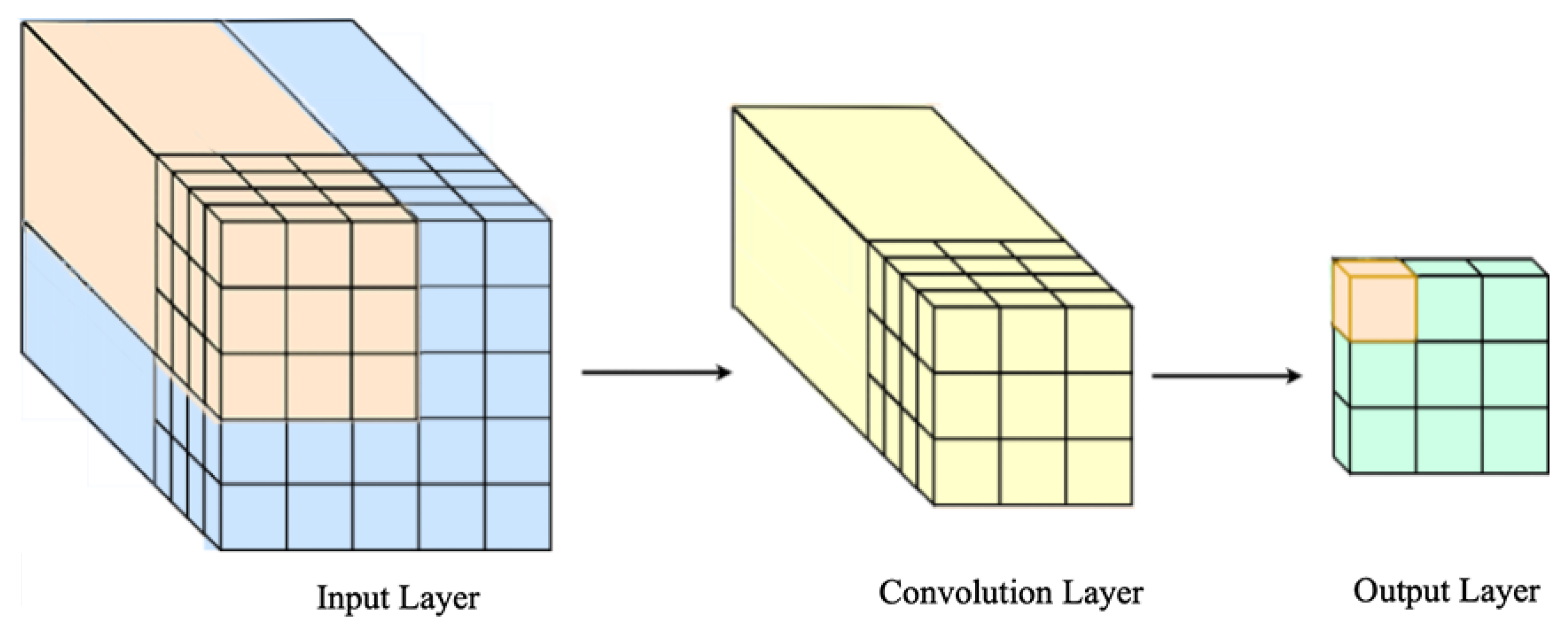
In Figure 3, sliding is performed at three positions horizontally and three positions vertically (3 = 5 − 3 + 1). After element-wise addition in the depth direction, one output channel is obtained.

Transformation is carried out between layers with different depths. Suppose the input layer has n channels, and the desired output layer has m channels. In this case, m windows need to be applied to the input layer, with each window having n kernels and providing one output channel. After applying m windows, there will be m channels, which are then stacked together to form the complete output layer. The m channels in the output layer are also referred to as m feature maps, so the number of output feature maps is the same as the number of convolution filters.

Although convolution is performed on 3D data (height × width × number of channels), it is still referred to as 2D convolution because the convolutional kernel moves only in the height and width directions. One filter and one image convolution can generate only one channel of output data, so the result is still in two dimensions.

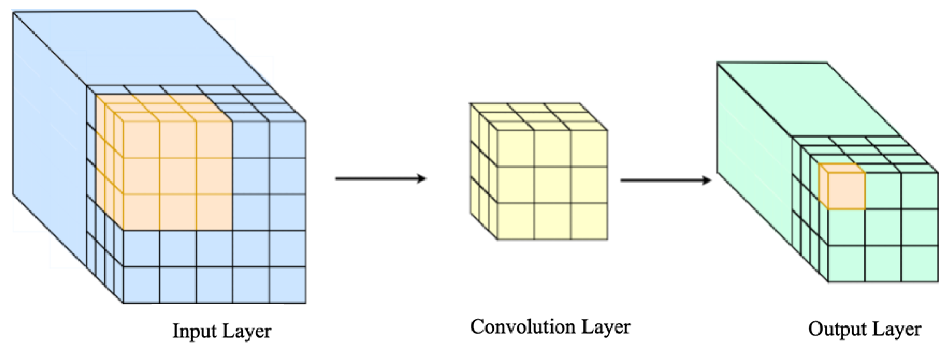
The data used in 3D convolution typically involve multiple 2D images stacked to form a 3D image, establishing spatial connections in the image.

Figure 4 illustrates the 3D convolution process. On the left is the input layer, where the convolutional kernel can move freely in three directions. The convolution is performed on each layer between two cubes, followed by element-wise addition in the depth direction, resulting in one datum and forming a plane. The convolutional kernel then moves in the depth direction, continuing the convolution, which outputs a 3D feature map.

The final output is a stack of green cubes, forming three channels of feature maps. Each feature map is no longer a plane but a three-dimensional cube. Here, we can observe that the number of output feature maps in the 3D convolution is still related to the number of convolutional kernels, but it should be referred to as the number of groups rather than individual kernels, as each group may contain multiple filters, and each group’s filter count equals the input’s number of channels.

2.2. Dynamic Convolution

However, 3D segmentation faces the challenge of higher computational resource consumption than 2D segmentation. Therefore, 3D segmentation algorithms usually downsample the input data [24]. This process can increase the network’s width, extracting richer details.

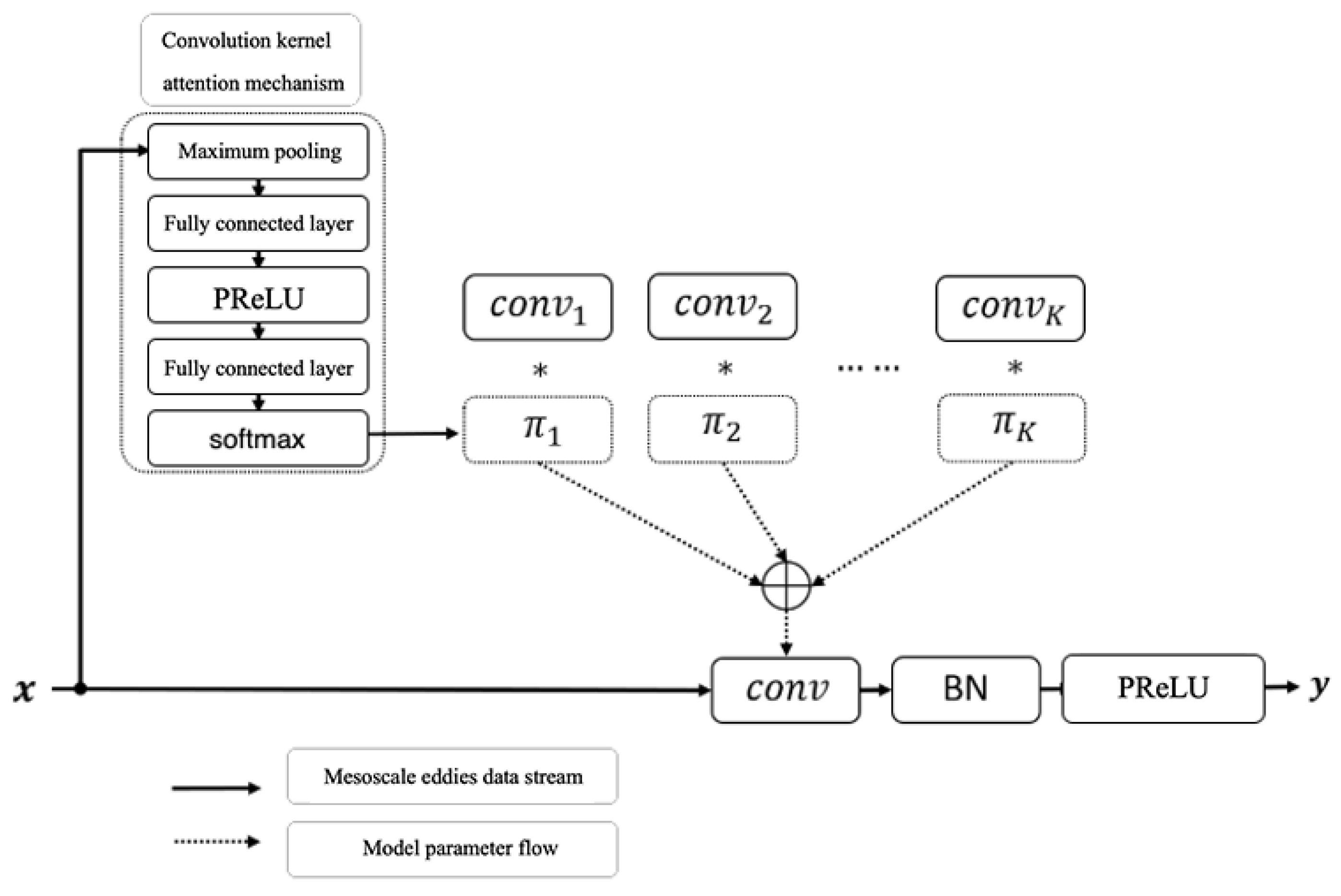
To cope with the constantly growing massive datasets, many researchers have attempted to improve model performance by increasing model complexity while maintaining stability to achieve higher accuracy. However, in 3D convolution, increasing model complexity significantly escalates computational costs. Dynamic convolution proposes a solution [25] by incorporating an attention mechanism in the convolutional kernel, enabling the network to adaptively generate different convolutional kernel parameters based on various input data. This balance between network performance and computational load enhances model robustness and accuracy.

Dynamic convolution achieves adaptability to different inputs by applying weights to the convolutional kernel. This is particularly important for inputting mesoscale eddy data, as such data exhibits diversity, including various information such as temperature, salinity, density, and velocity, which may influence the detection results. Combining temperature and salinity data with dynamic convolution helps mitigate network performance fluctuations caused by input data transformation.

Traditional convolutional layer designs usually employ static convolutional kernels. To enhance performance, model depth or width can be increased. Model depth can be increased by adding convolutional layers, fully connected layers, and activation function layers, while model width can be increased by enlarging the convolutional kernel size or input–output channel numbers. Although both methods can enhance model complexity and performance, they also consume more space and computational resources. Compared to traditional convolutional layers, dynamic convolution can adaptively generate convolutional kernel parameters, avoiding the limitation of fixed convolutional kernels, and better exploring features related to temperature, salinity, and other parameters in mesoscale eddy data. Additionally, dynamic convolution considers computational costs and spatial capacity during design. As a result, dynamic convolution not only improves model performance but also flexibly adapts to different task requirements while maintaining computational efficiency and space utilization.

In Figure 5, the parameters $con{v}_1$ to $con{v}_k$ are the convolutional kernel parameters obtained after the model’s initialization, and ${\pi }_1$ to ${\pi }_k$ are weighted coefficients learned through training, the ‘*’ means calculate. Different input data pass through pooling layers, fully connected layers, and PReLU activation function layers to generate weights, which are then multiplied and added to the convolutional kernel parameters to produce convolutional kernels suitable for static convolution. This design also takes into account computational costs and spatial capacity, allowing dynamic convolution to not only enhance model performance but also adapt flexibly to the demands of identifying three-dimensional morphological features of mesoscale eddies in the ocean while maintaining computational efficiency and space occupancy.

2.3. Residual Module

In the field of machine learning, enhancing the feature extraction capability of neural networks is crucial. One direct approach is to increase the depth of convolutional neural networks to enhance the model’s expressive power and classification performance. However, excessively deep networks can make training difficult and even lead to performance degradation. To address these issues, this paper introduces residual modules into the improved network model, effectively enhancing the model’s performance.

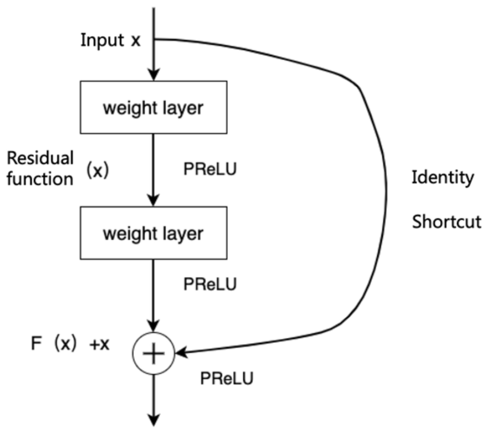
The residual learning module is a fundamental component of the ResNet network, consisting of a residual path and an identity path, as shown in Figure 6. It optimizes the training process with shortcut connections to prevent gradient vanishing and model degradation. The residual path comprises two sets of convolutional layers and a ReLU activation function, which are replaced with PReLU activation functions in this study.

The residual unit introduces skip connections, directly adding the input and output to complement the feature information lost during the convolution process. The output of the residual module is obtained by adding the residual path and the identity path, which helps prevent gradient vanishing and model degradation. This structure exhibits better optimization performance, as the shortcut connection structure does not increase computational complexity. Additionally, during the backpropagation process, the gradient is propagated to shallower layers through the skip connection structure, optimizing the training process. The network encoder of the residual structure consists of four groups of identical encoding blocks, each group including two convolutional layers and an activation function. One convolutional layer is responsible for computing the residual, while the other convolutional layer is responsible for extracting image features.

In the 3D-EddyNet network, the purpose of introducing residual modules is to learn new features while preserving the original ones. This enhances the feature extraction capability of the network without increasing computational complexity. This effectively addresses the problem of learning stagnation due to deep networks and ensures that the model does not suffer from performance degradation, thereby improving the network’s overall performance.

2.4. 3D-EddyNet

This research proposes a 3D-EddyNet model based on EddyNet and an improved U-Net network for three-dimensional mesoscale eddy recognition. To adapt to the three-dimensional recognition scenario, the model uses 3D convolutions instead of 2D convolutions to capture more spatial information. To address the challenges of increased computation and model complexity resulting from 3D convolutions, optimization strategies like the residual structure are introduced into the model. Additionally, dynamic convolution is incorporated to cater to multi-parameter inputs. These optimization strategies effectively alleviate network overfitting and gradient descent issues, leading to improved model accuracy and convergence speed.

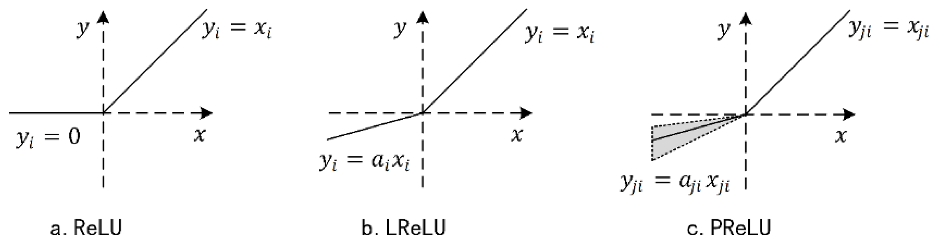
The Rectified Linear Unit (ReLU) activation function addressed the issue of vanishing gradients that could occur with sigmoid-based activation functions. Its design, based on neuron sparsity, ensured stable gradients, which benefited model training and improved convergence speed. However, ReLU had the drawback that weights could not autonomously update when the input was less than 0, potentially leading to gradient vanishing, reduced learning rates, and even the inability to learn meaningful features.

To alleviate this ReLU limitation, Maas et al. [26] introduced the Leaky Rectified Linear Unit (LReLU) as an alternative solution. However, LReLU’s performance strongly depended on the set slope parameter $\alpha$, making it challenging for practical applications. To address the issue of setting $\alpha$, He et al. [27] proposed the Parametric Rectified Linear Unit (PReLU) method. PReLU generated the hyperparameter $\alpha$ using a Gaussian distribution and automatically adjusted it during testing. The various activation functions are shown in Figure 7, demonstrating that PReLU significantly enhanced the training efficiency and accuracy of CNN.

Based on the aforementioned reasons, both the convolutional and hidden layers of the 3D-EddyNet model adopted PReLU activation functions. This choice not only fully utilized PReLU’s advantages in addressing the vanishing gradient problem and improving convergence speed but also circumvented the limitations faced by ReLU and LReLU, such as the inability to update weights when the input is less than 0. By using PReLU activation functions, the model could better learn meaningful features during the training process, thereby improving its performance. Furthermore, PReLU’s adaptive adjustment of the hyperparameter $\alpha$ provided the model with increased flexibility and robustness in real-world applications. As a result, the application of PReLU in our model ensured the improvement of training efficiency and the ability to handle complex problems.

In the 3D-UNet and V-Net models, the commonly used Dice loss function was utilized, which can mitigate the negative impact of foreground–background imbalance by focusing more on foreground regions and ensuring a lower false negative rate (FN). However, when dealing with scenarios with many small targets, the training process might suffer from oscillations. Furthermore, Dice loss is based on similarity comparison, making it unsuitable for the detection of mesoscale eddies.

In contrast, this study employed the cross-entropy loss function. This is a combination of softmax and cross-entropy loss functions. The smaller the cross-entropy value, the better the model’s performance, and its formula is shown in Equation (2):

$$H(p,q)=-{\sum }_{i=1}^{n}p\left(x_i\right){log}_{}\left(q\left(x_i\right)\right)$$

(2)

where p(x) represents the occurrence probability of time x, which is the true distribution of the samples, and q(x) is the predicted distribution.

Taking all factors into consideration, a network structure suitable for oceanic mesoscale eddy segmentation is constructed.

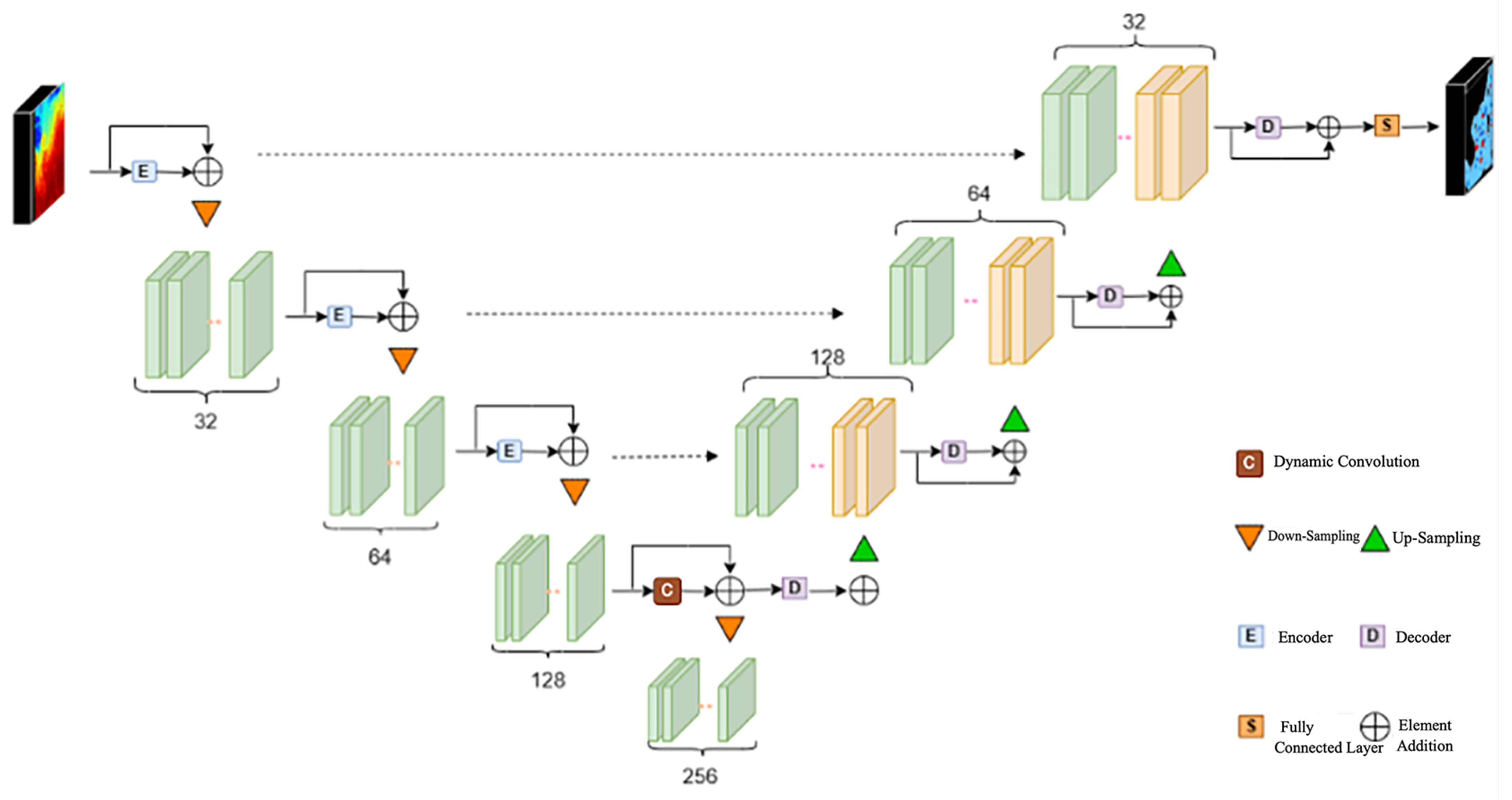
As shown in Figure 8, the 3D-EddyNet oceanic mesoscale eddy segmentation network structure consists of two parts: an encoder and a decoder, each containing convolutional layers and activation functions. The entire network structure fully considers the characteristics and challenges of oceanic mesoscale eddy recognition tasks. By introducing a series of optimization strategies and innovative designs, the model’s performance is enhanced, providing an effective solution for the automatic recognition of oceanic mesoscale eddies.

2.5. Training Optimization Strategy

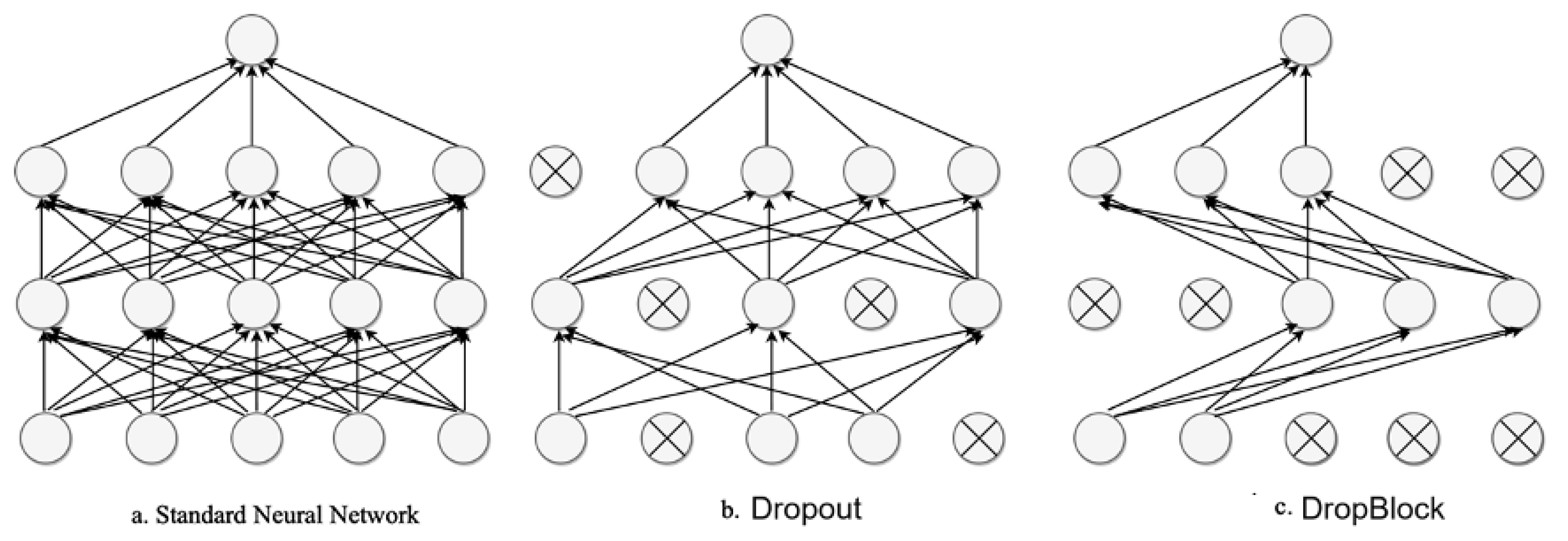
In the context of the limited availability of mesoscale eddy datasets, overfitting is a common concern. To address this issue, Dropout [28] is often introduced as a regularization technique to suppress certain feature co-adaptations and improve the network’s generalization ability. However, in three-dimensional convolutions, as the dimension of similar information increases, not only horizontal but also vertical correlations in the mesoscale eddy dataset cannot be ignored. Relying solely on Dropout may not achieve a satisfactory effect in mitigating overfitting. Therefore, this study employs the DropBlock module, which randomly deactivates specific regions to achieve information suppression and enhance network robustness, preventing overfitting.

DropBlock is an extension of Dropout to the convolutional layer. Its principle is simple, but it differs significantly from Dropout in that it masks a continuous block region, as shown in Figure 9.

DropBlock has two main parameters: block_size and $\gamma$. The $block\text{\_}size$ represents the side length of the block region, set uniformly for all feature maps regardless of their resolution. When $block\text{\_}size=1$, DropBlock approximates Dropout.

The parameter $\gamma$ controls the probability during the drop process, determining the number of blocked features and following a Bernoulli distribution. If the desired probability of keeping each activation unit is keep_prob, $\gamma$ can be calculated as follows:

$$\gamma =\frac{(1-kee{p}_{ratio})\times feature\text{\_}siz{e}^2}{(block\text{\_}siz{e}^2\times {(feat\text{\_}size - block\text{\_}size+1)}^2)}$$

(3)

The number of neurons to be dropped using DropBlock is given by the following:

$$(1 - kee{p}_{ratio})\times feature\text{\_}siz{e}^2$$

(4)

To ensure that DropBlock operates on the feature map, the block_size center needs to be at a certain distance from the feature map’s edge, which is $\left(block\text{\_}size\right)/2$. Therefore, the area where the block_size center is satisfied is as follows:

$$feature\text{\_}size-block\text{\_}size+1$$

(5)

Thus, the probability of DropBlock is

$$\gamma \times block\text{\_}siz{e}^2$$

(6)

The effective area for DropBlock is

$${(feat\text{\_}size - block\text{\_}size+1)}^2$$

(7)

Finally, the number of elements to be dropped is

$$\gamma \ast block\text{\_}siz{e}^2\times {(feat\text{\_}size - block\text{\_}size+1)}^2$$

(8)

To address the complexity and slow training speed of 3D-EddyNet, the Batch Normalization (BN) algorithm [29] was introduced to individually whiten each layer’s input in the neural network, transforming the image pixel values to a standard normal distribution with mean 0 and variance 1. This approach resolves issues related to uneven distribution and accuracy dispersion during training. Specifically, the BN operation is applied after the convolutional layer, normalizing the network responses for all data samples, and thereby mitigating the negative effects caused by uneven distributions and accelerating the training speed of the model, while simultaneously enhancing its precision and robustness.

Within 3D-EddyNet, each hidden layer’s output of a sample involves three dimensions. Therefore, the BN algorithm performs normalization for each dimension of every sample within 3D-EddyNet. This approach effectively improves the training performance of the neural network, expedites the convergence rate, enhances training efficiency, avoids overfitting, and maintains the network’s stability. By normalizing the network outputs, the BN algorithm aids in speeding up the convergence process, mitigating gradient vanishing or exploding issues during training, making the model easier to optimize, and improving the model’s adaptability to various inputs in real-world applications.

The model employs the PReLU non-linear activation function, which reduces the reliance on parameter initialization methods. However, suboptimal initialization can still negatively impact the training process. He et al. [27] proposed a novel parameter initialization strategy specifically optimized for ReLU activation functions and its variants, such as Leaky ReLU and PReLU. The main objective is to maintain appropriate signal magnitudes at each layer of the neural network during both forward and backward propagation, effectively alleviating the issues of vanishing or exploding gradients.

The concept behind this approach is that, in a PReLU network, half of the neurons in each layer are assumed to have a value of 0, while the other half are activated neurons. To ensure a stable variance, the method builds upon the Xavier initialization technique and divides the left-hand side of the variance derivation equation by 2. The weights of each layer are initialized from a Gaussian distribution with an expected value of 0 and a standard deviation of $\sqrt{\frac{2}{n_l}}$, where n_l represents the number of neurons in the lth layer. The He initialization method for PReLU is shown in Equation (9), where “a” is the tuning coefficient of PReLU.

$$W\sim N\left[0,\sqrt{\frac{2}{(1+a^2)n_l)}}\right]$$

(9)

In summary, 3D-EddyNet employs the He parameter initialization strategy to address the mentioned concerns effectively.

3. Data Sources and Dataset Construction

3.1. Data Selection

Mesoscale eddies in the ocean play a crucial role in absorbing energy from the larger background circulation and serve as significant peaks in the oceanic motion energy spectrum. Their kinetic energy profoundly influences temperature, salinity, and biogeochemical processes. However, accurately determining the three-dimensional morphology of these eddies presents challenges. Ocean altimeter satellites, including the French National Space Studies Center (AVISO), offer essential data support for large-scale and mesoscale eddy identification, particularly through sea surface anomaly height data. However, for studying subsurface structures, altimeter data alone is insufficient, necessitating the inclusion of sub-surface ocean temperature and salinity data.

The Argo program has been employed as an alternative approach, but its sparse and uncontrollable distribution of data points makes it challenging to fully represent the marine environment continuously. To address this, many research institutions grid and interpolate Argo data to create continuous oceanographic parameter data in the form of gridded Argo products, offering a more comprehensive understanding of the ocean’s state and variations.

Despite the benefits of gridded products, their spatiotemporal resolution often falls short of the requirements for mesoscale eddy identification. Their horizontal resolution is much greater than the average radius of these eddies, rendering them unsuitable. To overcome this limitation, high-resolution ocean model data, such as HYCOM, ROMS, and FVCOM, are employed, providing a satisfactory resolution for mesoscale eddy research.

HYCOM, in particular, is widely used due to its global coverage, versatility, and realistic representation of various ocean environments. Its hybrid vertical coordinate system allows for flexible stratification, making it well-suited for large open oceans with significant layering effects. FVCOM excels in nearshore regions, while the accuracy of vertical simulation results of ROMS is lower than that of HYCOM.

For this study, the GOFS 3.1 dataset (Global Ocean Forecast System 3.1) is adopted, representing one of the most advanced and high-resolution global volume grid systems in HYCOM. Compared to traditional grids, the volume grid system captures complex vertical structures more accurately, enabling better ocean forecasts and simulations. This dataset offers 41 layers of HYCOM and NCODA global spatial resolution of 1/12° and temporal resolution of 3 h, facilitating a comprehensive understanding of global ocean circulation, temperature, and salinity. The hybrid vertical coordinate system of HYCOM allows for a more precise representation of ocean features at different depths, including mesoscale eddies, enabling a better simulation of vertical movements and a more accurate capture of their three-dimensional structure.

The main purpose of this dataset is to understand and simulate global ocean circulation, temperature, and salinity. Helber et al. [30] employed an improved synthetic ocean profile to project surface information into the water column, resulting in global gridded high-resolution ocean data. HYCOM’s hybrid vertical coordinate system can more accurately represent ocean features at different depths, such as mesoscale eddies. This enhances the model’s ability to simulate vertical movements and better captures the three-dimensional structure of eddies.

The experimental area was selected as the South China Sea. Compared to open oceans, the South China Sea’s coastal currents are affected by the intrusion of the Kuroshio Current, complex seabed topography, monsoons, and other factors, resulting in more active and complex mesoscale eddy motion in the region; the surface circulation of the South China Sea exhibits rotational eddies [31].

The South China Sea is one of the largest semi-enclosed marginal seas in the western Pacific, with a complex ocean current system, and it exhibits a wealth of mesoscale eddy phenomena [32]. Figure 10, respectively, illustrates the sea surface temperature of HYCOM data at different times and depths.

3.2. Dataset Construction

The HYCOM model data cover global ocean regions. To reduce the data volume in the horizontal distribution, the South China Sea area is selected. However, in the vertical distribution, before the significant depth of 1000 m, there are six different intervals: 2 m, 5 m, 10 m, 25 m, 50 m, and 100 m. This uneven distribution hinders continuous identification. To improve the data content and make it more suitable for model detection, some data are discarded, and an interpolation algorithm is used to transform it into uniformly distributed input data at 50 m intervals. This interpolation process transforms the irregular mesh into a regular grid, facilitating model computations.

There are trilinear interpolation, inverse distance weighting, and kriging interpolation methods for comparison. Using HYCOM salt data from 2013 as the target dataset, we interpolated the data and compared them with the actual values to calculate the mean absolute error, relative error, and standard deviation. This allowed us to compare different interpolation methods. The results exhibited a slight advantage in terms of absolute error, relative error, and standard error, as shown in

Table 1. Average error statistics of interpolation method.

Methodical Error	Trilinear	IDW	Kriging
Absolute error	0.48	0.81	0.43
Relative error	1.61	2.72	1.46
Standard error	0.75	0.99	0.72

. However, this involves complex computations, taking into account not only the distance to the target point but also the spatial distribution and data points and considering the spatial correlation of variables. In scenarios with a large extent, Trilinear interpolation is a more effective choice.

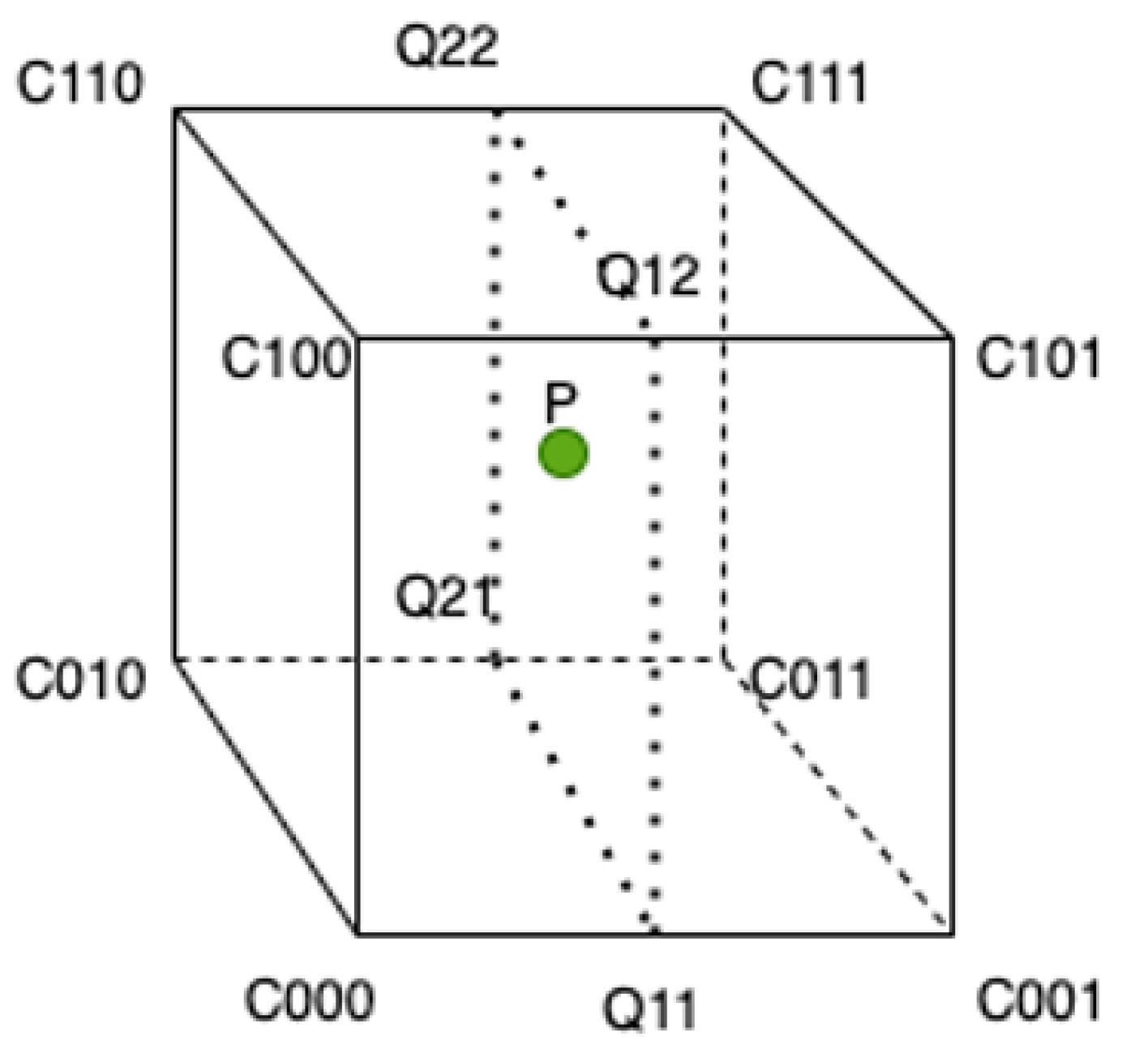
Trilinear interpolation is an extension of bilinear interpolation into three-dimensional space, essentially summing the weighted values of surrounding points for a specific point. Figure 11 illustrates the concept of the trilinear interpolation algorithm.

Given the green point P that requires interpolation, linear interpolation is used to obtain Q_11, Q_12, Q_21, and Q_22, which represent four neighboring pixel points, denoted as the lerp function. Assuming the differences between directions C001 and C000 are xd, the differences between C010 and C000 are yd, and the differences between C100 and C000 are zd, the values of the unknown function at these points are denoted as Value (x, y, z).

$$\left\{\begin{array}{c}Q\text{\_}11=Value\left(C000\right)\times (1-xd)+Value\left(C001\right)\times xd\\ Q\text{\_}12=Value\left(C100\right)\times (1-xd)+Value\left(C101\right)\times xd\\ Q\text{\_}21=Value\left(C010\right)\times (1-xd)+Value\left(C011\right)\times xd\\ Q\text{\_}22=Value\left(C110\right)\times (1-xd)+Value\left(C111\right)\times xd\end{array}\right.$$

(10)

After obtaining these four values, subsequent problems can be treated as classical bilinear interpolation. Combining with the initial dimension reduction process, the formula for calculating the value of point P is:

$$Value\left(P\right)=\left.\begin{array}{c}Value\left(C000\right)(1-xd)(1-yd)(1-zd)+Value\left(C111\right)xdydzd\\ +Value\left(C001\right)xd(1-yd)(1-zd)+Value\left(C011\right)xdyd(1-zd)\\ +Value\left(C010\right)(1-xd)yd(1-zd)+Value\left(C110\right)(1-xd)ydzd\\ +Value\left(C100\right)(1-xd)(1-yd)zd+Value\left(C101\right)xd(1-yd)zd\end{array}\right\}$$

(11)

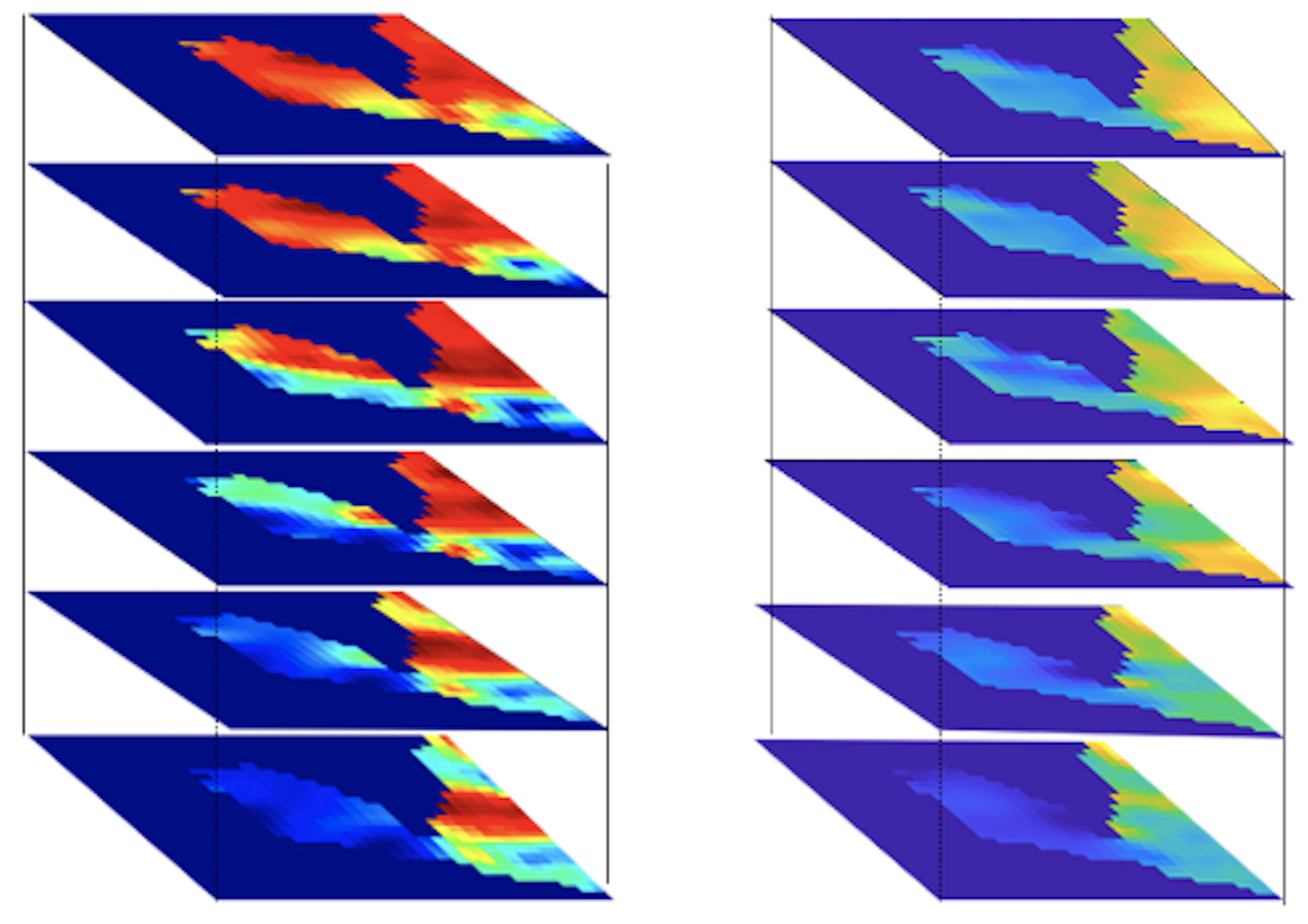
The result of linear interpolation is independent of the interpolation sequence. The post-interpolation result is shown in Figure 12.

After the interpolation, data from each depth layer are averaged, and the temperature and salinity anomalies are processed separately. The specific method involves calculating the average temperature and salinity at different depths and then subtracting the average values from the corresponding image pixels to obtain the anomaly data.

The Oceanographic Numerical Modeling and Observation Laboratory at Nanjing University of Information Science & Technology’s dataset is used as the two-dimensional labels for this study. This dataset is based on SLA (Sea Level Anomaly) data to detect the spatial distribution of mesoscale eddies in global ocean regions using the closed contour method of SLA anomalies. It also assigns attributes of −1 and 1 to distinguish between warm and cold eddies, as visualized in Figure 13 for different time periods.

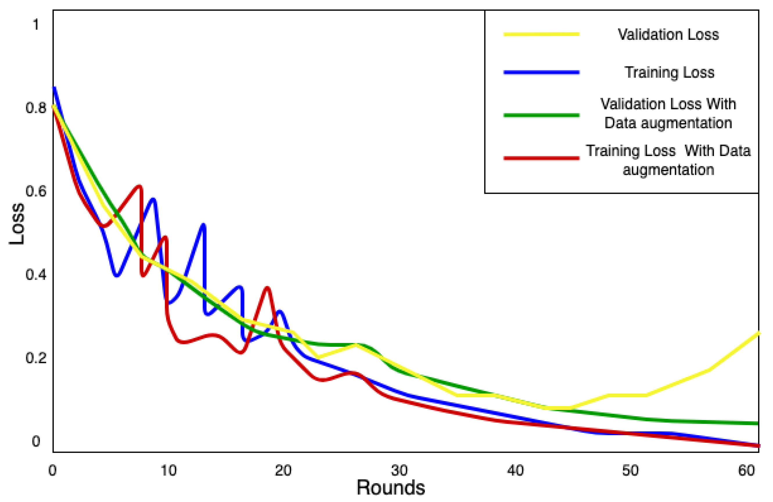
During the neural network model training, data augmentation techniques are used to improve the feature extraction capability of the 3D-EddyNet. Data augmentation, originally proposed by Dempster et al. [33], is a data expansion technique that aims to create as many useful data as possible from a limited set of mesoscale eddy data. Given the nature of neural network learning, it is crucial to maximize the volume of relevant data in the augmented dataset by leveraging the existing data. Supervised classification data augmentation involves applying predefined data transformation rules to augment existing data. This includes both single-sample data augmentation and multi-sample data augmentation. Due to the specific characteristics of HYCOM data, multi-sample data augmentation or color transformations are not suitable for this dataset; geometric transformations like mirroring and rotation are simple yet effective techniques within the single-sample data augmentation category. This enhances the quality of features extracted and avoids overfitting during the 3D-EddyNet training process, as shown in Figure 14; the validation set without data augmentation showed significant overfitting after 40 rounds.

Moreover, the dataset may lead to the poor generalization of new data; the dataset is partitioned into training, validation, and testing subsets based on their respective purposes. In this study, the data span from 1 January 1994 to 31 December 2012, with a spatial resolution of 1/12° and a weekly temporal resolution, covering a total of 19 years. Two data points per week, corresponding to the same dates as the label dataset, at 9 AM and 6 PM, are selected, and occasional missing data are supplemented with data from the preceding three hours, resulting in a total of 2086 HYCOM images. The dataset is divided into two categories: temperature and salinity. Data augmentation techniques, such as rotation and transposition, are employed to double the number of images. The dataset includes 15 years of data (1994–2008) as the training set, 2009 and 2010 as the validation set, and 2011 and 2012 as the test set. The training set contains HYCOM images with three-dimensional features of mesoscale eddies, while the label set provides information about the positions and categories of mesoscale eddies in each image.

4. Results & Discussions

4.1. 3D-EddyNet Model Ablation Experiment

The processed dataset has dimensions of 512 × 512 × 20. The original images are directly input into the network, and a process prediction is performed with a stride of 10. The output is then edge-processed, divided by four slices, and expanded outward by five pixels as a boundary processing method. Finally, the images are stitched together to form complete predictions.

The network model has 4 encoding stages, and the deepest layer has 32 channels. The input 3D data has dimensions of 512 × 512 for each layer, with a total of 20 layers. Due to the large memory usage of the original 3D input data, the neural network requires significant memory for feature extraction at each step. Memory is occupied by convolution layers, fully connected layers, BN layers, and other parameters, whereas activation function layers, Dropblock layers, and others do not have parameters.

In the HYCOM data product, mesoscale eddies are usually represented by closed contour lines. During the recognition process, the temperature and salinity anomaly isolines of connected regions are determined based on the network’s calculation results to identify the range of mesoscale eddies.

The evaluation of the results is done by comparing the output sea surface layer slice with the validation set pixel points. For the pixel points representing mesoscale eddies in the validation set, if the output result matches the segmentation ground truth, it is considered a true positive (TP); otherwise, it is a false positive (FP). For non-mesoscale eddy pixel points, if the output result matches the ground truth, it is considered a true negative (TN); otherwise, it is a false negative (FN).

Common segmentation metrics are used to evaluate the experimental results, including Accuracy, Precision, Recall, and $F_1$-Score. Compared with the 3D-UNet model, the proposed model in this study shows higher values in all evaluation metrics on both the training and validation datasets, as well as outperforming network models without the addition of optimization modules. However, the classification results show a difference of over 10% compared to the validation set, indicating a relatively large error. This may be due to the type of data in the label dataset, which are MSLA sea level anomaly data that inherently carry some errors when compared to the HYCOM data used in this experiment. The specific parameters are listed in

Table 2. Comparison of model segmentation effects.

Model	Dataset	Accuracy	Precision	Recall	${\mathit{F}}_1$-Score
3D-UNet	Training set	89.93	89.06	89.71	89.38
	Validation set	86.05	87.54	86.30	86.94
3D-UNet+ Residual module	Training set	91.21	90.76	90.51	90.63
	Validation set	88.22	88.11	88.28	88.19
3D-UNet+ Dynamic convolution	Training set	90.93	91.06	90.72	90.88
	Validation set	87.65	87.54	88.30	87.92
3D-EddyNet	Training set	93.47	92.53	91.84	92.18
	Validation set	89.82	89.14	90.03	89.57

.

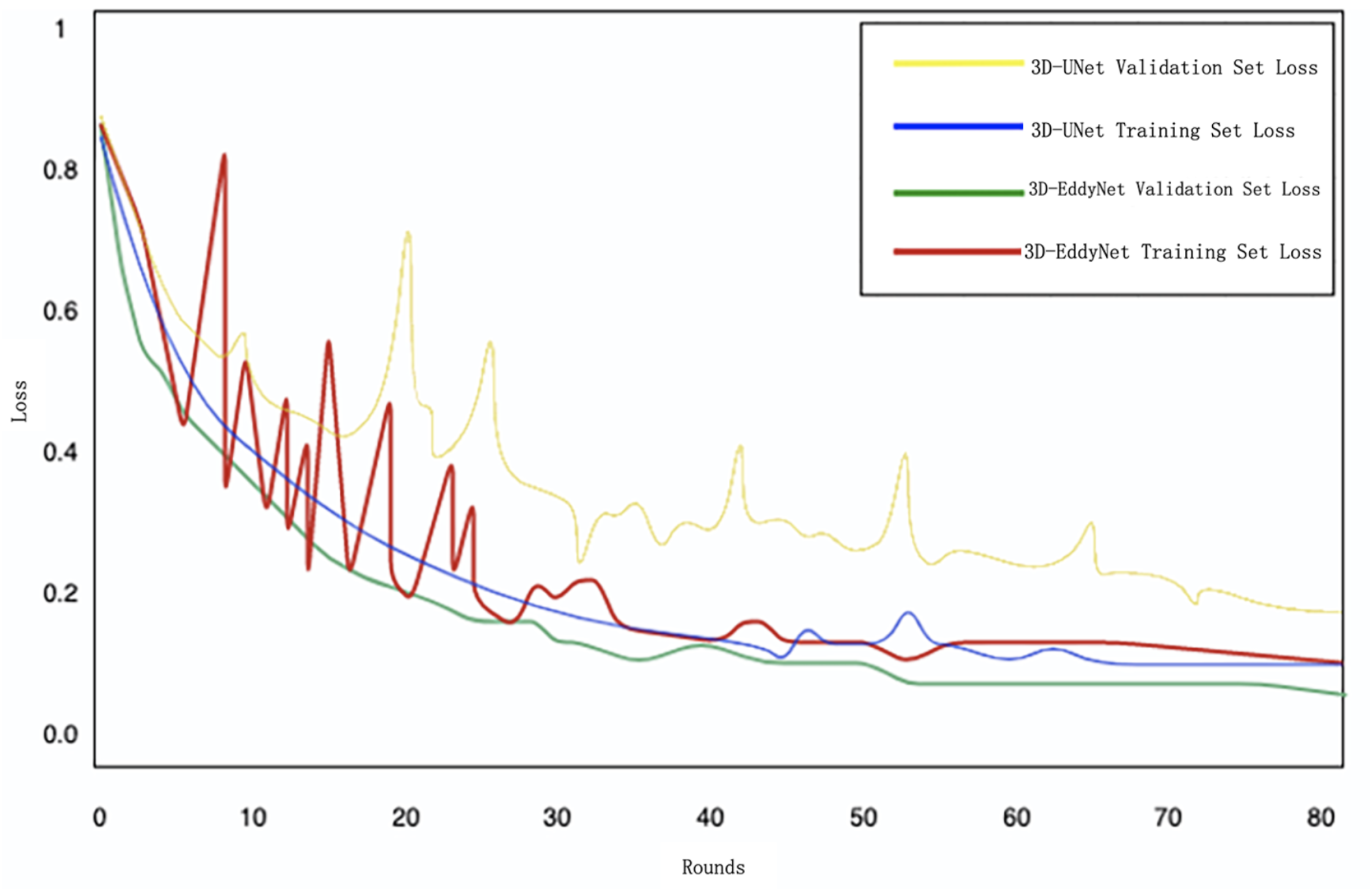
Furthermore, the loss accuracy curves of the two models are analyzed. When using the 3D-UNet network for comparison training, the training loss gradually decreases, and the learning rate also decreases continuously. The final loss values converge to around 0.2. The training set generally stabilizes around 60 epochs out of 80, while the validation set’s loss continues to decrease, but with some oscillations.

After incorporating the neural network training optimization strategy mentioned earlier, the training loss changes, as shown in Figure 15. Generally, faster convergence speed, smaller oscillations, and lower loss values indicate better network performance. The proposed model in this study achieves significantly lower loss values compared to the 3D-UNet model and converges faster, stabilizing around 50 epochs.

In the early stages, the training set experiences relatively intense fluctuations, which gradually decrease over time, and later, the network parameters are optimized, and the learning rate decreases, leading to overall stability in the curve. By comparing the results, it is evident that the optimization module improves training effectiveness, resulting in improvements in model accuracy and speed, surpassing the 3D-UNet model.

Therefore, a comprehensive analysis of segmentation performance, detection accuracy, convergence speed, and other factors reveals that the proposed network in this study demonstrates superior performance and exhibits better mesoscale eddy detection effectiveness.

4.2. Temporal and Spatial Distribution Characteristics of Mesoscale Eddies

Between 1994 and 2012, the South China Sea experienced a varying number, size, and three-dimensional morphology of mesoscale eddies. On average, there were 35.2 ± 2.5 eddies in the region per image, with approximately 52% being Cyclonic Eddies (CE), characterized by clockwise rotation in the southern hemisphere (high-pressure center) and counterclockwise rotation in the northern hemisphere (low-pressure center). The remaining 48% were Anticyclonic Eddies (AE), exhibiting the opposite rotation pattern.

Spatially, mesoscale eddies were widespread in the South China Sea, exhibiting a general northeast–southwest distribution. Regions with higher eddy occurrence were observed near the southwestern part of Taiwan, southwestern part of Luzon Island, and northeastern part of Natuna Island, especially in the area from southern Taiwan to the northern Philippines (Luzon Island). In this region, the volume of mesoscale eddies was significantly larger than in other areas, likely due to its unique geographic location and topographical conditions. Overall, the western South China Sea was a region with high eddy occurrence, where approximately 28% of the eddies were observed west of 113° E, while only 13% were located east of 116° E. The distribution of CE and AE was similar in most areas, with a tendency towards AE in many regions. Notably, areas near the Luzon Strait showed higher eddy occurrence and exhibited specific eddy shapes, suggesting a possible relationship between mesoscale eddy formation and seafloor topography.

In terms of temporal distribution, mesoscale eddies were present throughout the year, but the total number varied significantly among different months, showing a close correlation with seasonal changes. In spring and autumn, mesoscale eddies were more abundant than in summer and winter. During spring, AE predominated in the eastern waters of Taiwan near the equator, as well as in the vicinity of the Luzon Strait. This was related to the active spring monsoon, enhancing the presence of AE in these regions. In summer, due to the influence of the summer monsoon, AE was mainly observed in the western waters of Luzon Island, while CE was distributed in the northeastern part of the South China Sea, where eddy activity was more apparent. In autumn, a small number of CE appeared in the eastern waters of the Philippine archipelago, while AE, similar to spring, was widely distributed in the Luzon Strait and its adjacent areas, showing a distinct regularity. During winter, a higher number of CE was generated in the northeastern waters of Natuna Island and the vicinity of the Luzon Strait, while AE was mainly distributed in the eastern part of Luzon Island, the central basin of the South China Sea, and the central waters of the Philippines.

The variation in the number and distribution of mesoscale eddies throughout the year is significantly influenced by the monsoons, which introduce periodicity in the regions with intense eddy activity.

In 2012, the average number of mesoscale eddies detected per month was analyzed and presented in Figure 16, showing the monthly variations.

Regarding the three-dimensional morphology of the eddies, a statistical analysis was performed, revealing that most of the eddies were located above 800 m (85.4%), with the core situated above 600 m (78.1%). Approximately 69% of the eddies had radii smaller than 50 km, and the average horizontal radius was less than 40 km. Above 100 m, AE had slightly larger total pixel area and average radius than CE, while below 300 m, the situation reversed, with CE having larger pixel area and average radius. The spatial distribution of eddy pixel values indicated that larger eddies were more prevalent in the northeastern and western parts of the South China Sea. The depth of 600 m acted as a turning point, with CE’s dominance exceeding AE’s in numbers above this depth. This further confirmed the dominance of CE at various vertical levels.

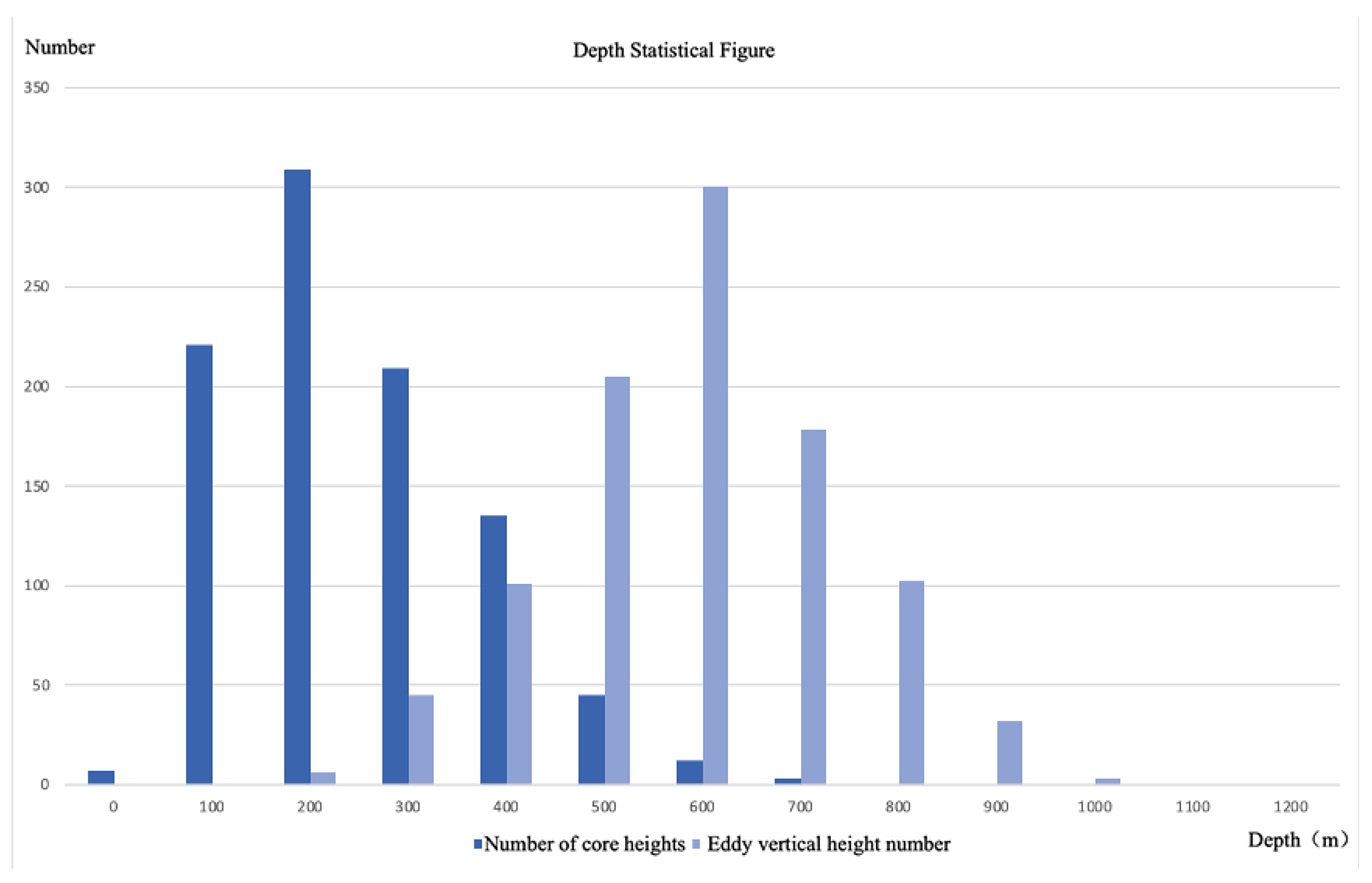
Regarding the eddy radii statistics, to eliminate seasonal effects, weekly images from 2012 were taken, and statistical analyses of the eddy radii and vertical depths were performed. The relationship between the core position and the number of eddies with depth is shown in Figure 17. The results demonstrated that eddy cores were mainly located at depths between 100 and 300 m, while eddies were generally observed at depths exceeding 1000 m. The eddy radii gradually decreased with depth, with AE exhibiting higher numbers and larger average radii than CE above 200 m, while below 200 m, CE had more significant numbers and larger average radii than AE, consistent with the previously described patterns. This aligns with the findings of Lin [14] in their statistical analysis of mesoscale eddy data in the South China Sea. The number of CE and AE in different depth ranges showed a particular trend: CE dominated above 350 m, while below 350 m, AE became more prevalent.

4.3. Three-Dimensional Shape Analysis of Mesoscale Eddies

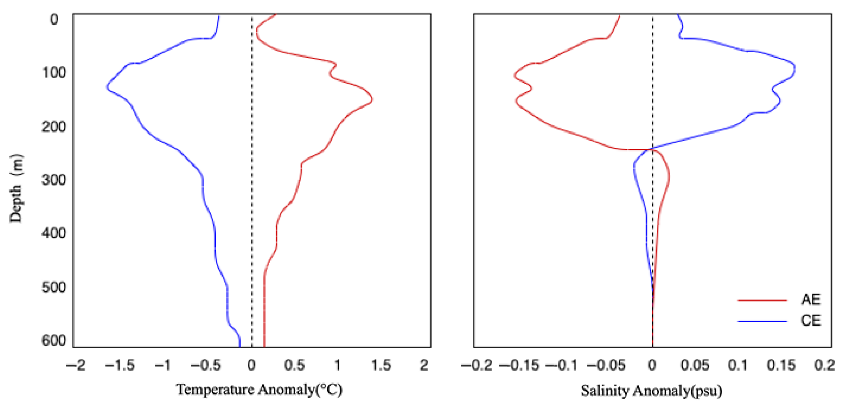
Regarding the three-dimensional morphology analysis, the temperature and salinity anomalies in the dataset were combined and processed to obtain the composite average temperature and salinity anomalies of eddies with depth. The results showed that the temperature anomaly peaked at 110 m in the center of the composite CE and at 100 m in the center of the composite AE. The temperature anomalies for CE and AE were approximately −1.6 °C and 1.5 °C, respectively, while the salinity anomalies were approximately 0.15 psu and −0.17 psu. The structures of temperature and salinity anomalies exhibited differences, with temperature anomalies often vertically extending between 300 and 500 m, while salinity anomalies were primarily confined to the upper 200 m, with a counter-directional movement near 300 m.

The identification results are in line with He’s conclusions [18], showcasing that eddies exhibit elongated conical shapes within the range of 60 m to 90 m. Temperature and salinity anomalies also attain their peaks at the core of eddies, measuring 1.5 °C and 0.15 psu, respectively, in cyclonic eddies, and 1.4 °C and 0.16 psu in anticyclonic eddies. Temperature and density anomalies extend vertically to the depth of 400–500 m, while salinity anomalies are discernible only within the upper 150 m, further substantiating the effectiveness of 3D-EddyNet, as is shown in Figure 18.

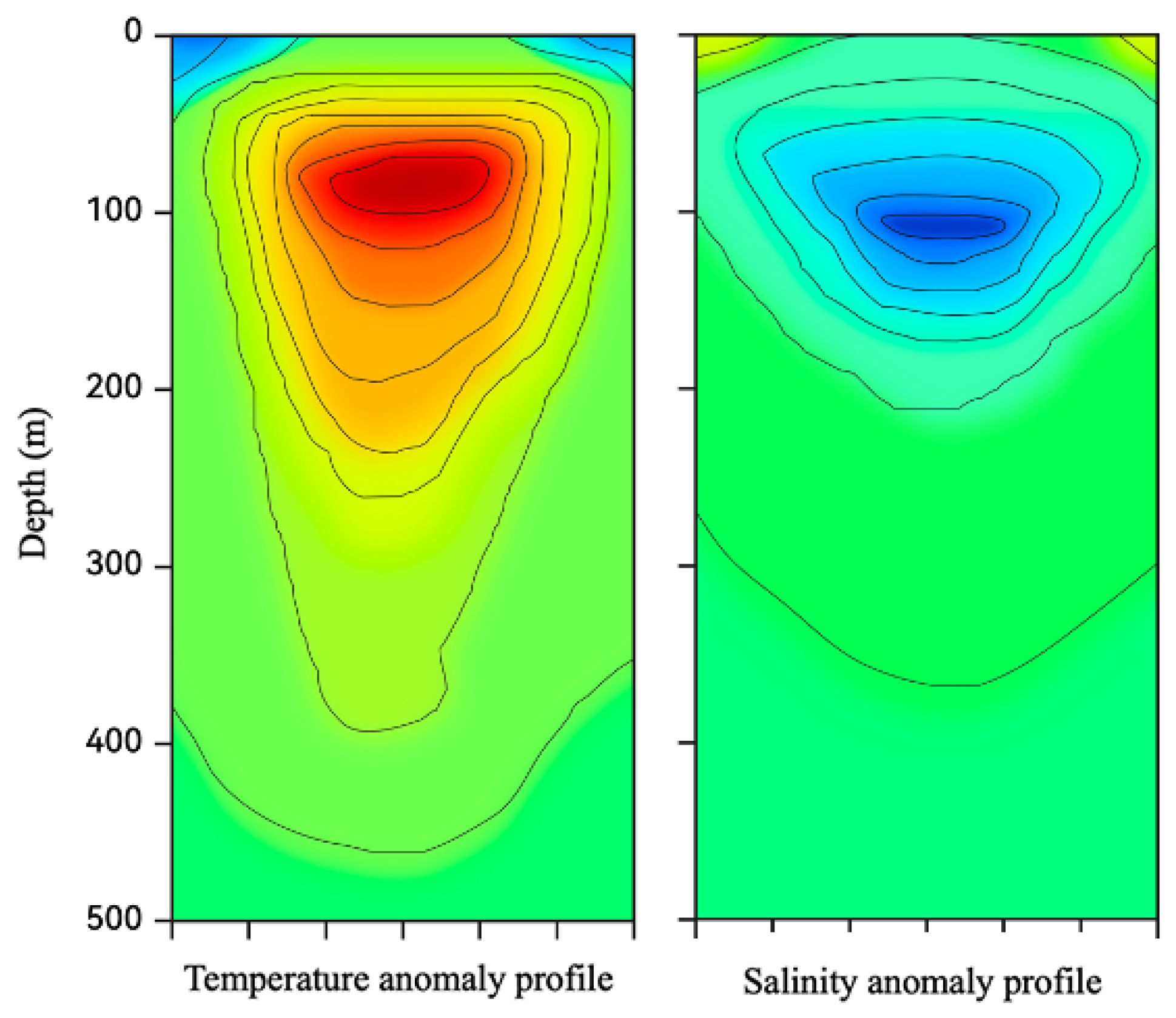
The salinity anomaly profiles and cross-sections exhibited distinct differences from the temperature anomaly profiles and cross-sections, as shown in Figure 19.

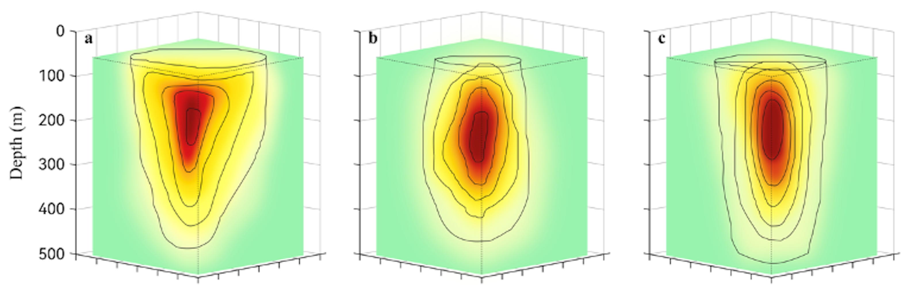
To visualize the results, the mesoscale eddies in the South China Sea were categorized into three main forms based on their vertical depths: top-enhanced bowl-shaped eddies, middle-enhanced olive-shaped eddies, and bottom-enhanced near-cylindrical eddies, as shown in Figure 20.

However, there are discrepancies between the identification results and the actual ocean conditions. These discrepancies arise because the model data may differ from real ocean data, and the current data label set is still two-dimensional, affecting the accuracy of three-dimensional feature recognition and potentially overlooking sub-surface eddies. As a result, the size and vertical extent of eddies cannot be fully captured, leading to significant differences from the real situation.

In the realm of oceanography, a multitude of complex phenomena intricately influence marine dynamics. These phenomena include internal waves, ENSO, and mode waters. 3D-EddyNet observed the impacts of these phenomena on the mesoscale characteristics of the ocean to varying degrees, aiding in the exploration of interrelationships among various phenomena. Furthermore, if efficient and accurate methods for excluding the impact of specific phenomena on observational results can be identified, it would further enhance the practicality of our model.

5. Conclusions

In this study, we propose a 3D-EddyNet model based on a three-dimensional neural network, which effectively addresses training issues related to recognition efficiency, accuracy, and gradient degradation, enabling efficient and accurate identification of mid-scale eddy morphology.

3D-EddyNet overcomes the limitation of previous deep learning methods in recognizing mid-scale eddies, as it can extract features beyond the sea surface. By filling the gap in deep learning approaches for identifying three-dimensional morphological features of mid-scale eddies, this model enhances our understanding of the ocean and provides a fundamental basis for studying material transport patterns in ocean dynamics and safeguarding the marine environment.

The discrepancies between real ocean and data affect the identification results of eddies, thereby impacting the overall research negatively. To improve the accuracy of the validation method, it is essential to wait for more comprehensive data and introduce three-dimensional standards for validating and analyzing the results, ensuring that the conclusions drawn are closer to the actual conditions and enhancing the reliability and accuracy of the research.This article primarily centers on introducing the methodological research.

Furthermore, the identification method primarily relies on detecting anomalies to determine the shape, depth, radius, and other features of abnormal regions, but it cannot explore the internal details and structure of eddies. Therefore, it is hoped that researchers will use more suitable datasets and incorporate physical ocean knowledge and other parameters to analyze the internal structure of eddies in future studies.