1. Introduction
In underwater detection tasks, autonomous detection based on sidescan sonar (SSS) images [
1,
2,
3,
4] plays a crucial role in the field of underwater intelligence due to its wide detection range and high imaging accuracy for underwater substrates. Among traditional detection methods and deep learning-based approaches, deep learning-based object detection has demonstrated significant advantages. Compared to traditional methods that suffer from poor robustness, high algorithm design complexity, and subpar detection performance, deep learning-based methods, when given sufficient training data, achieve superior detection results without these limitations, making them the most popular approach for autonomous detection. Our team previously conducted research in the domain of applying lightweight neural network models to semantic segmentation tasks in sidescan sonar image analysis [
5]. We have also released relevant models, some of which are utilized in this paper. Our primary aim was to further optimize these models to enhance their accuracy, optimize their speed, or reduce their parameter count. However, upon experimentation, we encountered a significant limitation imposed by the available dataset. The performance of the models on datasets with ample ground-based data far surpassed their performance on datasets with relatively limited underwater data. As a result, we redirected our focus towards acquiring a more extensive dataset. However, in underwater detection, the collection of SSS data is extremely challenging and costly, especially in marine environments. The insufficient amount of data severely hampers the development of underwater autonomous detection techniques. Therefore, generating and augmenting limited data to meet the requirements of deep learning algorithms is crucial.
Generative adversarial networks (GANs) are a category of deep learning-based generative models designed to harness the essence of human-inspired creative processes. The core idea involves training generator and discriminator models in a competitive manner using two deep neural networks to generate samples resembling real data. Since their inception in 2014 [
6], GANs have made remarkable progress in overcoming the bottleneck of pattern generation in various domains, such as images, audio, and text. Many research teams have contributed significantly in this field; for example, Chen T et al. [
7] suggest a framework to offer orthogonal gains to existing real image data augmentation methods and additionally presented a new feature-level augmentation that could be applied together with them. Xu L et al. [
8] introduced a GAN-based transformer for general action-conditioned 3D human motion generation, including not only single-person actions but also multi-person interactive actions. Chai X et al. [
9] proposed a robust compressed sensing image encryption algorithm based on a generative adversarial network, a convolutional neural network (CNN), a denoising network, and a chaotic system.
Moreover, GANs have achieved great success in various domains. In image processing, GANs are widely used for generating and restoring images of faces, scenes, and Renaissance styles [
10,
11]. In the field of speech, GANs are utilized for generating high-quality speech samples and speech recognition [
12,
13]. In natural language processing, GANs are employed to generate text content with good semantics [
14,
15].
Despite the numerous advantages of GAN networks, two significant problems exist: gradient vanishing and mode collapse. These issues make it difficult for GAN networks to converge, requiring extensive parameter tuning to obtain good results. In order to address these problems, Radford et al. [
16] proposed the WGAN network model, and Ishaan Gulrajani et al. further improved it by introducing WGAN-GP [
17], effectively alleviating the aforementioned issues. The mainstream GAN networks are now built upon this design basis. A new method called Markov chain conditional pix2pix (MC-pix2pix) has been proposed in the field of underwater detection [
18] to generate realistic SSS images, and MC-pix2pix data were used to train autonomous object detection networks. Another study [
19] presented a semantic image synthesis model based on pix2pix, reconstructing SSS simulation images from simple hand-drawn segmentation maps of target photos. This approach can generate sonar images at different water depths and frequencies. However, the application of GAN networks in underwater detection remains relatively rare, and there are few datasets of sonar images that are rich in substrate features suitable for semantic segmentation.
By building upon prior research, the proposed substrate classification architecture is designed for application to a limited SSS dataset. This architecture employs a neural network model grounded in the principles of WGAN-GP. It encompasses the generation of raw data and the preliminary labeling of sample labels. Image feature processing methods are then employed to reduce image noise and enhance the clarity of the generated images. Subsequently, the usability of the generated data is assessed through experiments, and the enhancement in substrate semantic segmentation performance is evaluated.
The main contributions of this study are as follows:
1. A network model is formulated in accordance with WGAN-GP principles for the purpose of sidescan sonar (SSS) image segmentation. The model’s architecture is tailored to accommodate the distinctive characteristics of various environmental regions;
2. Image feature processing algorithms are applied to mitigate image noise and enhance the perceptual clarity of the generated images;
3. An encoder-decoder-based semantic segmentation network model is established and trained using unprocessed data to conduct preliminary autonomous labeling on the generated data. Subsequently, through manual refinement, the labeled dataset is reintegrated into the training pipeline, culminating in enhanced semantic segmentation performance on authentic data;
2. Related Work
Within this section, the exploration of pivotal concepts in model design ensues. These encompass the foundational principles underpinning GANs, the WGAN-GP variation, and the methodology of segmentation.
2.1. GAN Model
Generative adversarial networks (GANs) operate on the fundamental principle of pitting two networks against each other: a generator and a discriminator, which are engaged in competitive interplay. The generator’s role is to persistently create samples, endeavoring to render it challenging for the discriminator to differentiate between the generated and genuine samples. Conversely, the discriminator’s objective is to enhance its discriminative prowess by accurately discerning whether an input is authentic or generated. Through this adversarial dynamic, the generator strives to produce samples that progressively mimic real ones, whereas the discriminator grapples with increasing difficulty in distinguishing between them. Eventually, as the generator improves, it learns the distribution characteristics of real samples and generates new samples that exhibit authenticity. The objective function of the GAN network is defined as follows:
In the given context, the symbol x represents authentic data, whereas signifies the output produced by the discriminator network. Typically, this output is a scalar value denoting the proximity of the input to genuine data. represents the input provided to the generator network, denoted as G, and represents the resultant output generated by the generator.
The primary objective of the discriminator network is to differentiate between real and synthetic samples. Specifically, when presented with a legitimate image, denoted as
, the discriminator should assign a high score, aiming to maximize
. Conversely, when confronted with images generated by the generator
, the aim is for the discriminator
D to allocate a low score, with the objective of minimizing
. Therefore, the objective function of the discriminator network can be expressed as
The objective of the generator is to maximize the score assigned by the discriminator, which is equivalent to minimizing
. Thus, the objective function for the generator can be written as
The combination of these objectives leads to the overall objective function of the GAN network. It has been proven that this function has a unique optimal solution [
20].
2.2. WGAN-GP
Training a GAN can be challenging as it often encounters various problems, with three major issues listed as the following:
(1) Gradient vanishing: This often occurs when the discriminator is too good, hindering the improvement of the generator. When using an optimal discriminator, training can fail due to gradient vanishing, resulting in insufficient information for the generator’s improvement.
(2) Mode collapse: This refers to the phenomenon where the generator repeatedly produces the same output or a small group of outputs. If the discriminator gets trapped in a local minimum, it becomes easy for the next generator iteration to find the most reasonable output according to the discriminator. The discriminator never learns to escape this trap.
(3) Convergence failure: Due to various known and unknown factors, GANs often fail to converge.
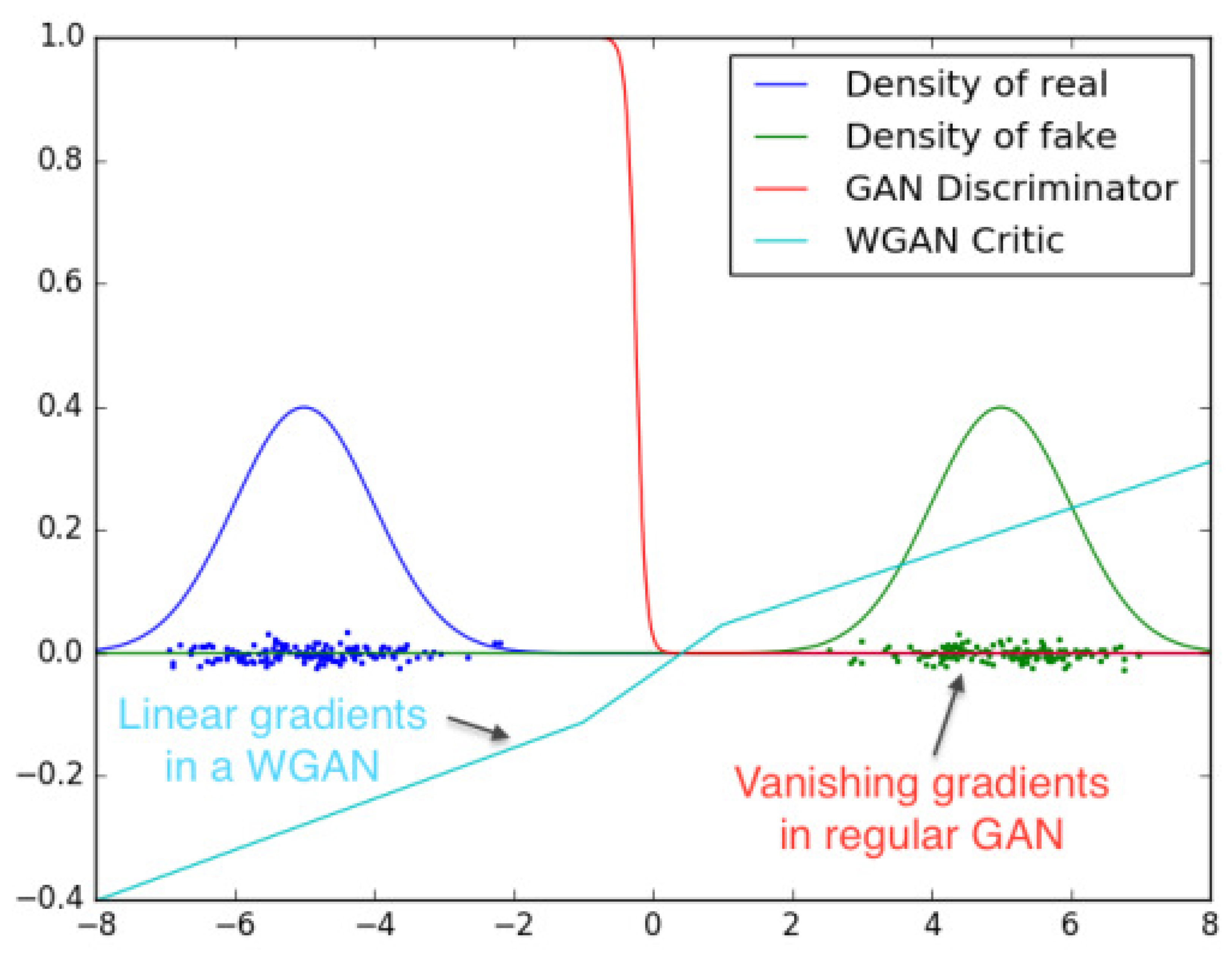
Wasserstein GAN (WGAN) makes a simple modification by replacing the Jensen-Shannon divergence loss function with Wasserstein distance (also known as Earth Mover’s (EM) distance) in traditional GANs(showed in
Figure 1). The GAN network aims to make the generated and real data distributions as close as possible, with the objective of minimizing the Jensen-Shannon divergence. By optimizing the Jensen-Shannon divergence, the network pulls the generated distribution closer to the real distribution, ultimately generating highly similar data. This concept holds when there is some overlap between the two distributions in their initial states. However, if the two distributions have no overlapping parts or the overlapping parts are negligible, the Jensen-Shannon divergence remains constantly at log2, and the model becomes trapped in an optimization problem.
The key solution lies in using Wasserstein distance to measure the distance between the two distributions. Wasserstein distance has the advantage that it can reflect the distance between two distributions even when there is no overlapping area.
Assuming that we want to transform probability distribution p to q and define the distance function (transportation cost) as d(x,y), then the Wasserstein distance is defined as [
16]:
where
represents the joint distribution of
p and
q.
The authors of WGAN derived and transformed the traditional GAN formulation based on Kantorovich-Rubinstein duality.
L represents the network function, represents the distribution of real data, and represents the distribution generated by the model.
However, to satisfy the Lipschitz constraint, WGAN constrains the parameter values in the network. Even with this constraint, when stacking multiple layers in the model, gradient vanishing and explosion can still occur. WGAN-GP introduces an additional regularization term based on the WGAN objective function [
17]:
The latter half is the regular term, represents data generated by the model, and this term is the gradient penalty (GP) in WGAN-GP, which enforces the gradient constraint. The constraint implies that the L2 norm of the critic’s gradient relative to the original input should be close to 1 (bilateral constraint). This constraint ensures better training performance while preserving the Lipschitz constraint.
2.3. Semantic Segmentation
The realm of semantic segmentation tasks boasts a range of noteworthy models, including DeepLabV3 [
21], hrnet [
22], and Transformer [
23]. However, the foundational concept behind segmentation models traces back to the inception of fully convolutional networks (FCNs). FCNs introduced a pivotal paradigm shift by substituting fully connected layers with fully convolutional layers for generating activation outputs. This transformation entails a shift from a simplistic, one-dimensional probability vector output to a more sophisticated two-dimensional probability matrix output, facilitating pixel-level segmentation accuracy.
FCN’s innovation also encompassed image size restoration via deconvolution operations, coupled with the incorporation of skip connections. The integration of these skip connections, bridging high-dimensional and low-dimensional features, exerted a profound influence on subsequent semantic segmentation models. In the wake of FCN’s pioneering work, the U-Net model emerged as another influential milestone. U-Net departed from the usage of VGG networks as the backbone and instead introduced a symmetrical encoder-decoder architecture comprising four layers. Additionally, U-Net incorporated cascaded connections between each layer of the encoder-decoder structure.
The decision to forego deep networks as the backbone proved to be an effective strategy in mitigating overfitting, particularly in scenarios characterized by limited dataset sizes. Even today, U-Net continues to find applications in contexts with restricted sample sizes, such as medical image segmentation.
3. Method
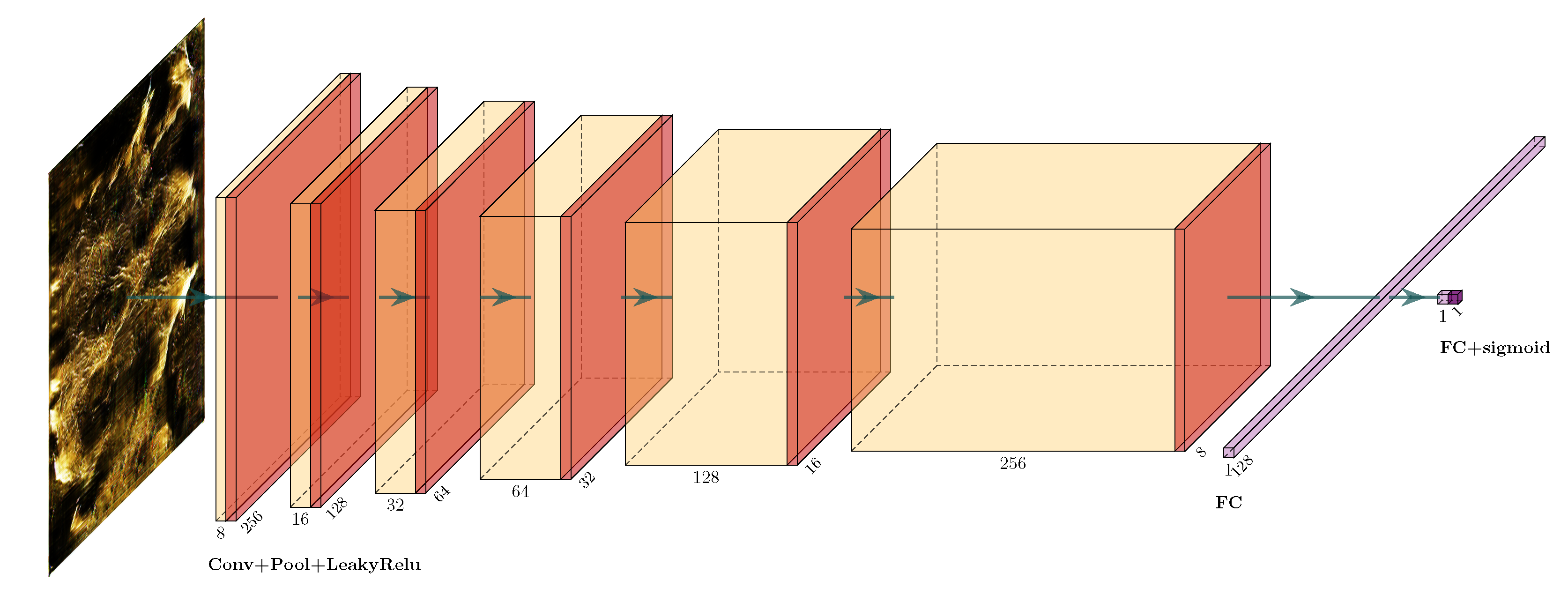
A generator model and a discriminator model have been meticulously devised, both relying on multi-layer convolutional neural networks. The generator adopts a forward-stacked convolutional neural network architecture, featuring a gradual reduction in the number of channels in each layer, ultimately producing RGB images with three channels as output. Conversely, the discriminator progressively increases the number of channels in each layer, culminating in the last layer’s transformation through a fully connected layer to yield the judgment result.
Following this, a semantic segmentation network model was formulated, drawing inspiration from the U-net architecture for the autonomous labeling of generated images. This network incorporates multi-scale convolutional kernels, multi-link parallel structures, and the integration of attention mechanism modules. After undergoing training with genuine images, the generated images underwent an initial phase of autonomous labeling.
3.1. Image Generation Model
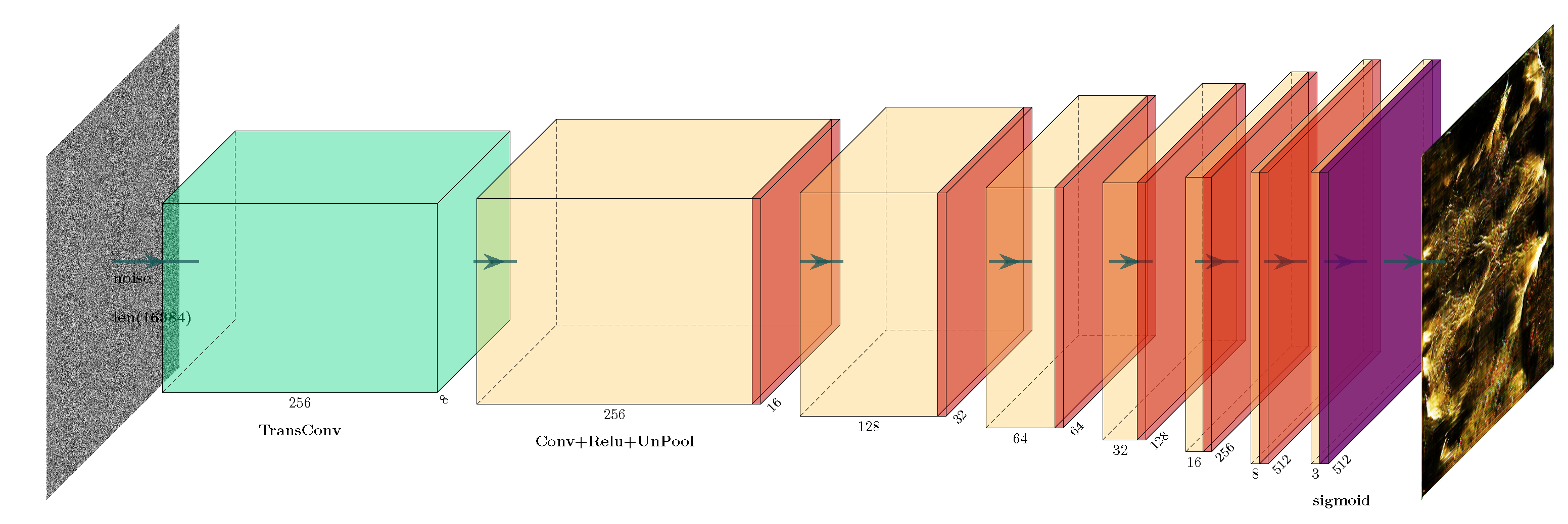
The image generation network was devised within the WGAN-GP framework, and its architecture is depicted in
Figure 2 and
Figure 3.
The generator’s structure begins with a one-dimensional Gaussian noise vector as input. Since the input image size is large, the first two layers of the network apply 7 × 7 convolutions for deconvolution, followed by a ReLU activation function. The following layer sequence is repeated six times: convolutional layer, batch normalization layer, ReLU activation, and upsampling layer. For the first and second iterations, the filter size of the convolutional layer is 4 × 4, while for the remaining parts, the size is 3 × 3. Finally, after the convolutional layers, a sigmoid activation function is applied. The result of this layer sequence is an image with a size of 256 × 256.
The discriminator takes previously generated images from the generator as input and applies a series of layers. This layer sequence is also repeated six times: convolutional layer, batch normalization layer, ReLU activation, and average pooling layer. All convolutional layers of the discriminator use a 3 × 3 filter size. Finally, a fully connected layer followed by a sigmoid activation function is used as a binary classifier.
3.2. Feature Enhancement
Images generated by GAN networks have some deficiencies in terms of clarity, size discrepancies with the original image, and lack of smoothness. Feature enhancement is needed to address these issues. Initially, image smoothing is achieved by the construction of a Laplacian image pyramid. The Laplacian pyramid is grounded in scale-space theory and Gaussian filters, entailing a two-step implementation process: downsampling and upsampling. In the downsampling phase, the original image is subjected to Gaussian smoothing, yielding a sequence of scaled images with distinct sizes and varying degrees of blurriness. Subsequently, in the upsampling phase, the Laplacian pyramid generates higher-resolution images by computing the differences between adjacent scale images.
Within the Laplacian pyramid’s construction process, Gaussian filtering is first applied to the input image, yielding a succession of scaled images.
represents a Gaussian filter, and
i denotes the scale (scaling factor) of the image. The downsampling process can be achieved by retaining every kth image in the Gaussian pyramid, where
k is a multiple factor controlled by the scale coefficient. Subsequently, an upsampling process is performed on the Gaussian pyramid, followed by taking the difference between adjacent images.
Here, U denotes upsampling, which is performed using bi-cubic interpolation to enhance clarity and enlarge the image. Through this process, a Laplacian pyramid can be generated, where each level is represented by a pair of vertically and horizontally differentiated images. By blending the differential images with the original image, the image can be smoothed.
The post-smoothed image reduces singular values but also exhibits a certain degree of quality degradation. Therefore, image sharpening is required. Unsharp masking (USM) is a commonly used image enhancement algorithm that sharpens the image by computing the difference between the original image and its Gaussian blur, thus improving image clarity. The mathematical formula for this algorithm is
Here, USM
represents the enhanced pixel value of the image,
represents the pixel value of the original image,
represents the pixel value of the Gaussian blurred original image, and
k represents the enhancement coefficient. The specific
can be expressed as follows:
where
N represents the size of the Gaussian blur,
K represents the weight parameter,
represents the weight value of the Gaussian filter, calculated using the following formula:
Here, is the standard deviation of the Gaussian filter.
3.3. SE-Block and Attention
The SENet [
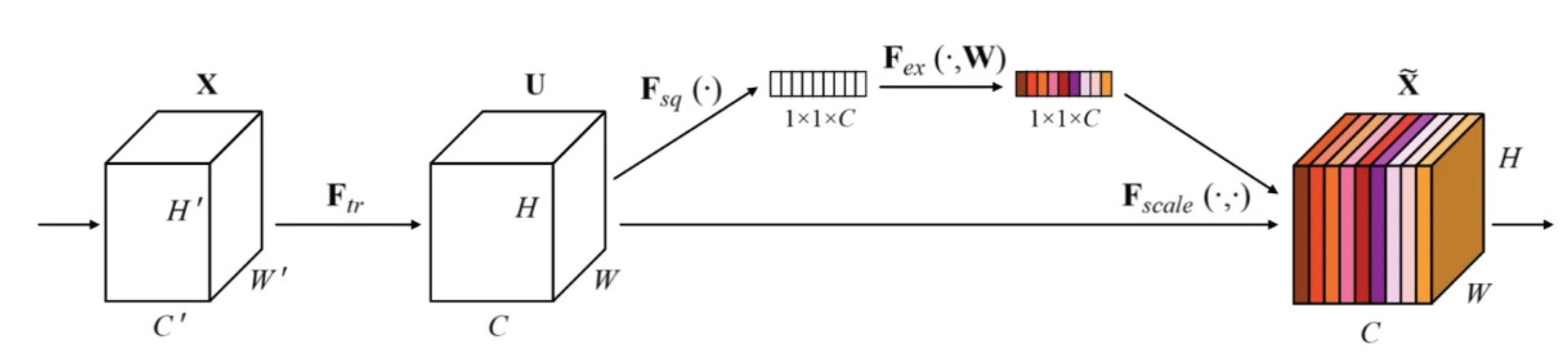
24], which secured the championship in the 2017 ImageNet competition, is a significant model in computer vision. It is formally known as the Squeeze-and-Excitation Congestion Network, and its notable contribution lies in the incorporation of a channel attention extraction module referred to as the Se-Block. This module possesses the flexibility to be seamlessly integrated into various network architectures (showed in
Figure 4).
The Se-Block comprises two integral components: first, the squeezing module, responsible for condensing the initial 3D input data into a one-dimensional vector. This operation is primarily achieved through global average pooling, facilitating the extraction of global characteristics from each channel. Second, the excitation module employs a fully connected layer to transform the output of the squeezing module into a predictive weighting sequence. This sequence is then applied as weights to all channels, effectively emphasizing crucial channel features while downplaying less significant ones.
3.4. Autonomous Label Generation Model
A semantic segmentation neural network model was meticulously crafted and trained, utilizing authentic data as the foundational source for automated label generation.
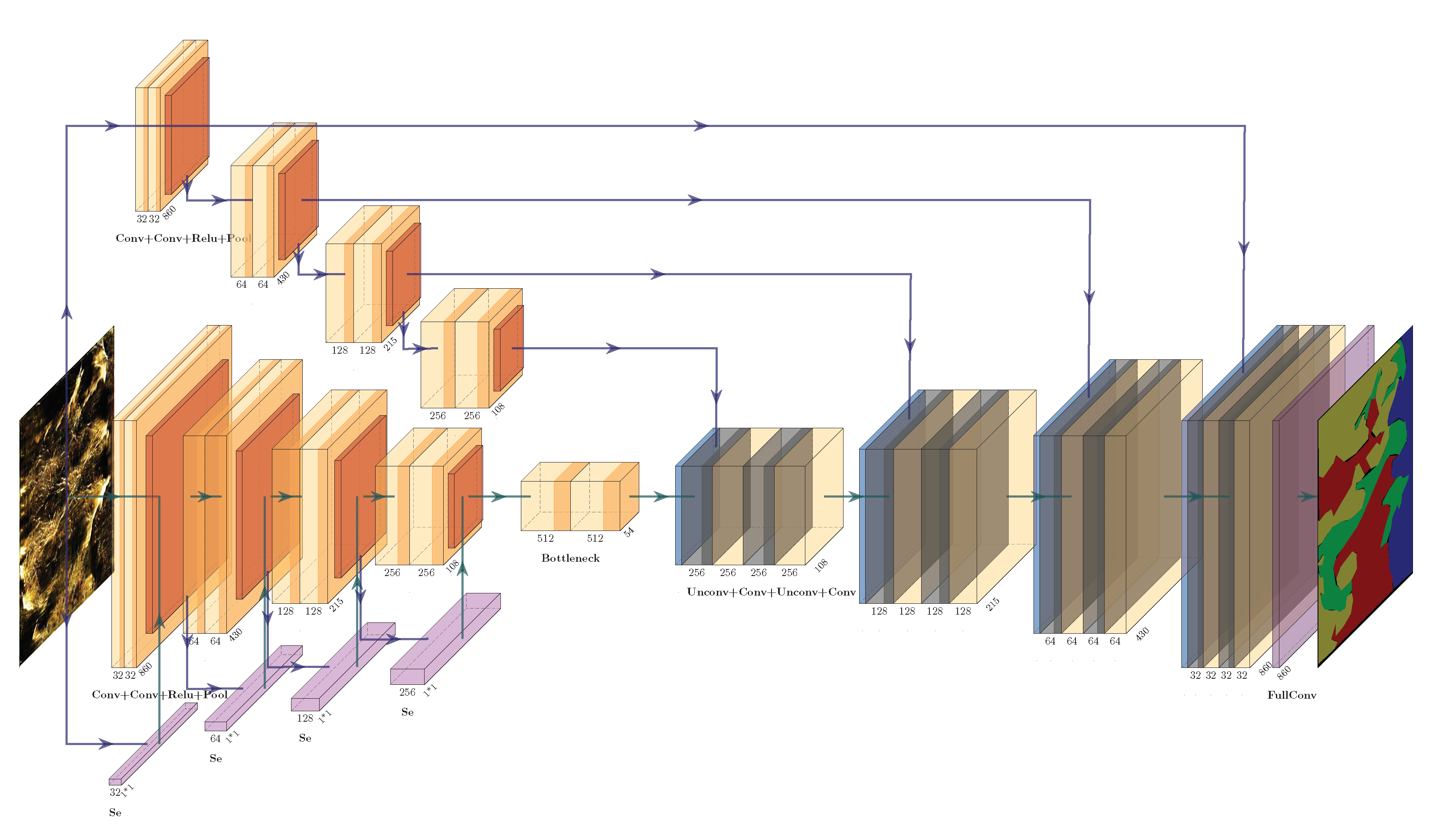
The architectural configuration of our model is elucidated in
Figure 5, comprised of both an encoder and a decoder, each comprising four layers akin to the U-Net architecture. The data undergoes an initial denoising step before entering the encoder, where feature extraction is performed. This is accomplished through the deployment of four parallel feature extraction modules, with each module dedicated to processing one of the RGB channels from the original input image.
Within each feature extraction module, there are four layers, and these layers encompass two feature extraction modules each, incorporating a 7 × 7 convolution kernel size. Notably, for the sake of maintaining image size through padding, conventional convolution is replaced by depthwise (DW) convolution. The encoding blocks utilize 7 × 7 convolution kernels, again employing DW convolution to enhance computational efficiency while preserving padding. The number of output channels for each layer is systematically set at 32, 64, 128, and 256. Additionally, SE (Squeeze-and-Excitation) blocks are seamlessly integrated into each layer, facilitating the prediction of channel weights.
Another distinct input pathway consists of the entire set of channels originating from the original input image. In this scenario, each layer comprises two feature extraction modules employing a 3 × 3 convolution kernel size, and conventional convolution is utilized. The number of output channels for each layer mirrors the configuration of the other three modules.
When moving forward, the decoder phase commences by taking the 512-channel heatmap output generated by the bottleneck module, which is subsequently reduced to 256 channels via upsampling. These channels are then concatenated with the data derived from the fourth module, a process facilitated by the application of small convolution kernels, resulting in the acquisition of a 512-channel feature map. This process iterates four times, culminating in the final segmentation outcome achieved through a fully convolutional layer.
4. Experiment and Analysis
The experiments were conducted on a computing system comprising an Intel Core i9-10900F CPU running at a clock speed of 2.8 GHz (20 cores), 64 GB of RAM, an NVidia Geforce 3090 GPU with 24 GB of video memory, and utilizing CUDA Toolkit 11.3, CUDNN V8.2.1, Python 3.6, and PyTorch-GPU 1.10.1, all running on the Ubuntu 18.04 operating system.
4.1. Dataset Collection
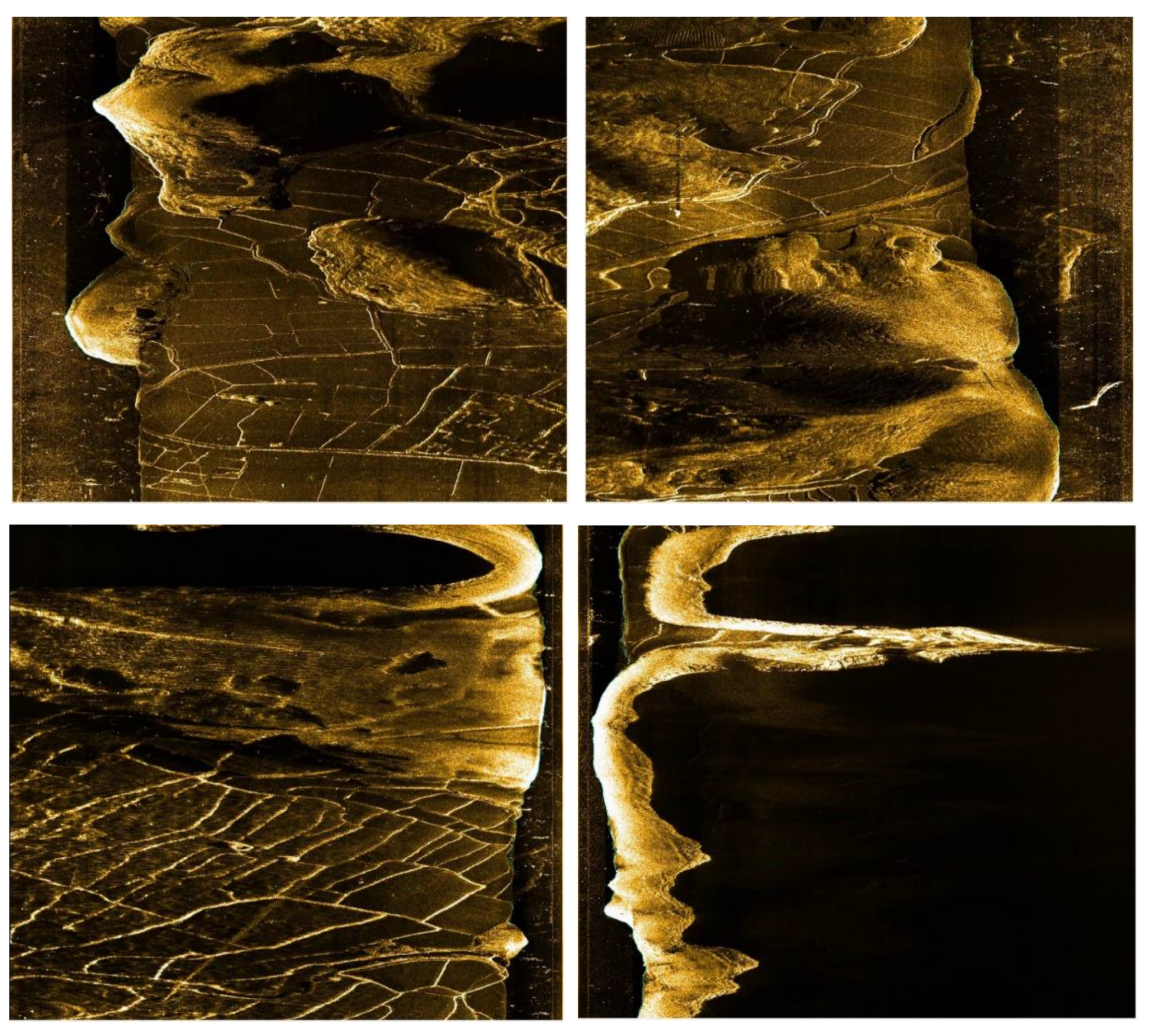
In the course of our experimental investigation within the Jiande Lake District, located in Hangzhou, China, we utilized the Hydro 3060 dual-frequency sidescan sonar to acquire crucial sonar data. The original images obtained sequentially in a frame-by-frame fashion, possessed dimensions of 960 × 960 pixels, as depicted in
Figure 6, serving as an illustration of their quality.
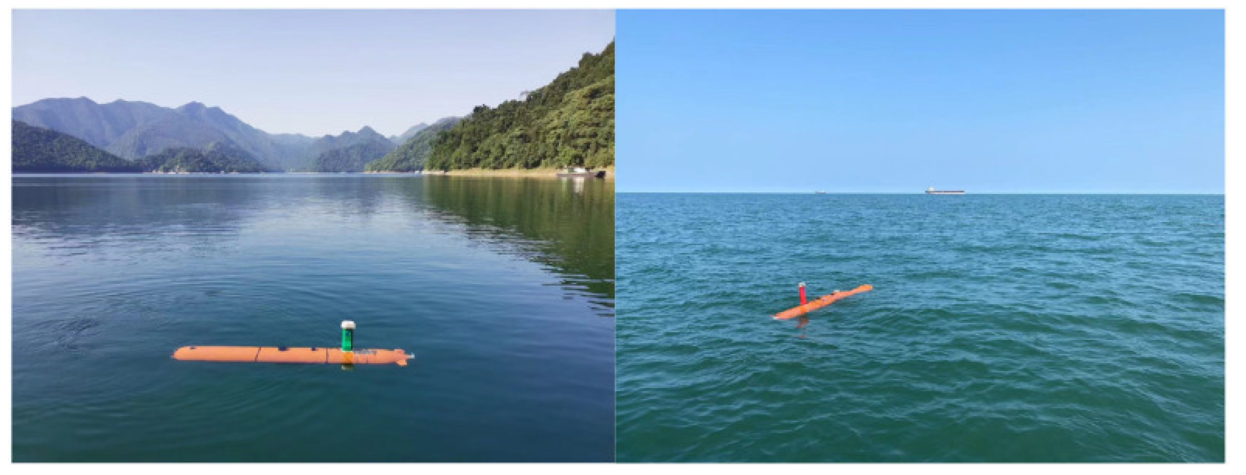
When mounted onto an autonomous underwater vehicle (AUV), as depicted in
Figure 7, the sidescan sonar emits acoustic waves in lateral directions while the vehicle is in motion. This process involves the reception of echoes from submerged objects, enabling the construction of an imagery representation. Within the resulting imagery, the regions characterized by strong echoes, such as rocks and metallic objects, manifest as bright areas, whereas the regions devoid of echoes, such as bodies of water and obstructed sections, appear darkened.
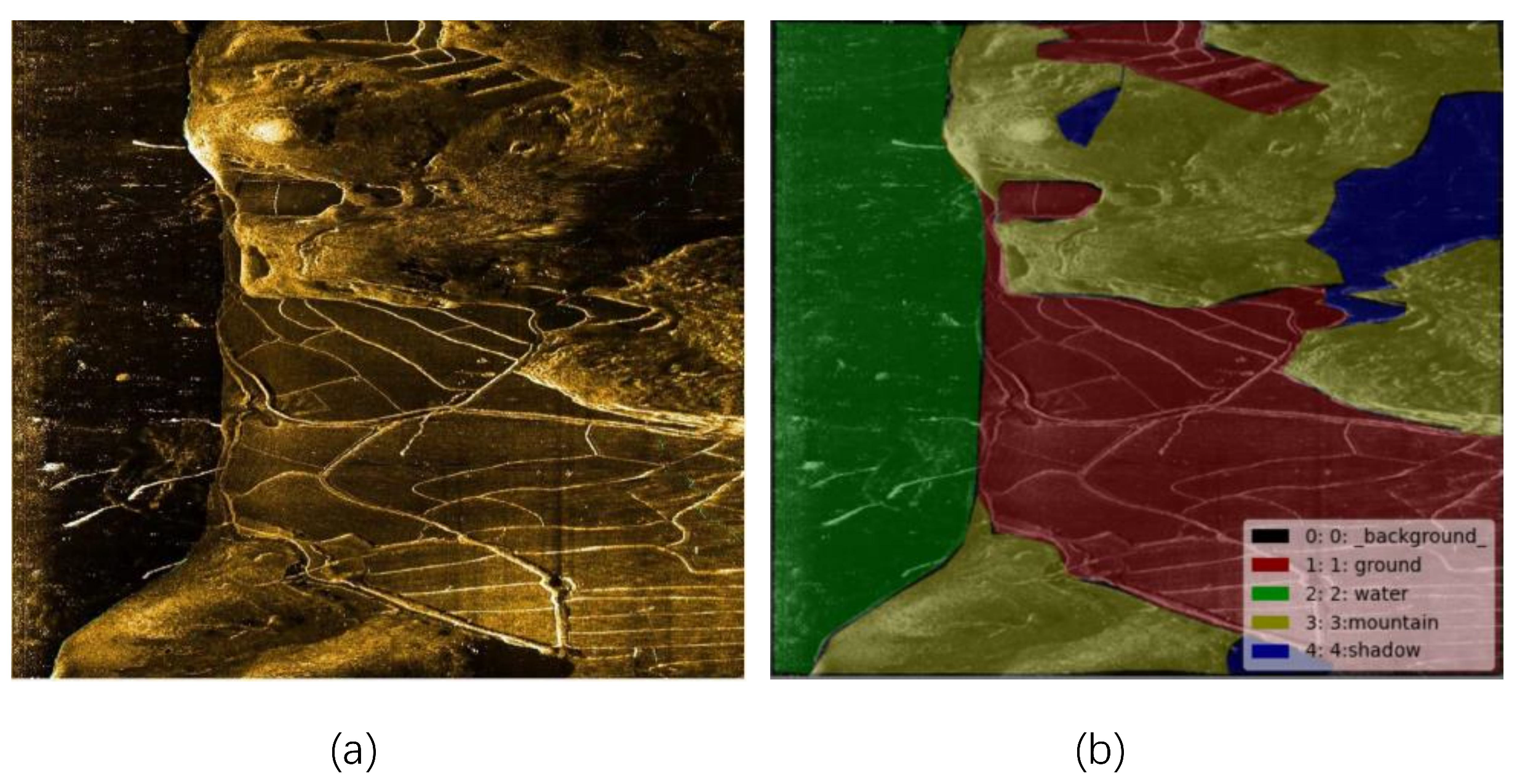
Our model is rooted in supervised learning, necessitating the availability of meticulously annotated and accurate data labels for training. Data annotation was conducted using the open-source software LabelMe, which was implemented by using the Ubuntu platform. The entire dataset was categorized into five distinct classes (although not every image encompassed labels from all five categories): (1) Water; (2) Mountainous regions; (3) Land areas; (4) Shaded portions; (5) Unmarked regions (background). The designation of "unmarked area" primarily pertains to the residual debris regions remaining after the initial labeling of the first four image types. A visual representation of a labeled image is presented in
Figure 8.
4.2. Data Augmentation
As previously mentioned, the acquisition of sidescan sonar data poses challenges, resulting in a relatively limited dataset. In order to address this limitation and enhance training efficacy, we employed data augmentation techniques as follows:
Image Flipping: The conventional approach involves horizontally flipping the images at various angles. This augmentation method not only increases the dataset size but also disrupts location-based correlations, promoting a more generalized network.
Image Translation: Another standard technique entails controlled image translations in four directions using random adjustments, albeit within reasonable bounds. Excessive translations are avoided to prevent the distortion of image feature structures.
Random Cropping: Data augmentation was further facilitated by randomly cropping sections from the original images. This reduces the image size while expanding the dataset and expedites training.
Notably, for sonar images, the emphasis is placed on color features rather than shape characteristics; hence, color-based data augmentation was not pursued. The original sonar data had dimensions of 960 × 960 pixels and consisted of approximately 300 samples. Following data augmentation, the data were resized to 860 × 860 pixels, effectively increasing the dataset size by a factor of approximately four. For training purposes, a random selection comprising 60 percent of the augmented data was allocated as the training set, whereas the remaining 20 percent each constituted the validation and test sets.
4.3. Data Generation
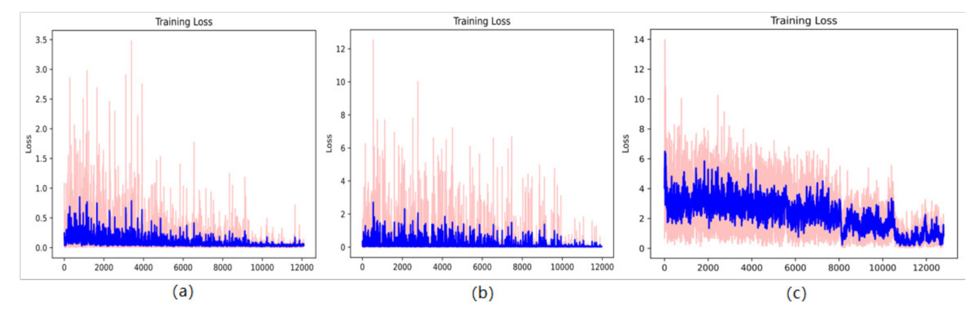
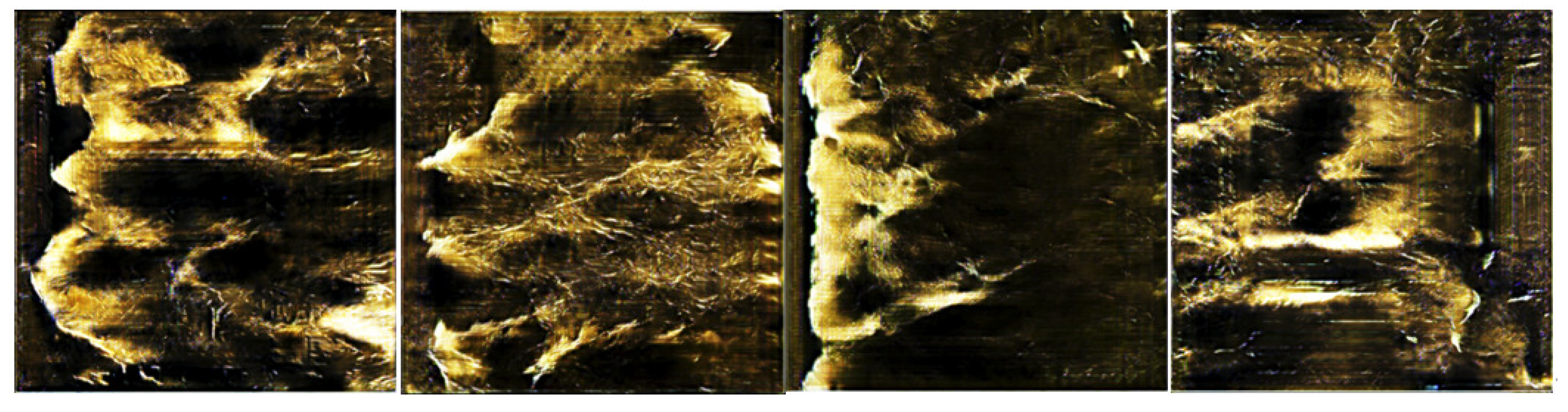
About 80 percentof the real sonar images were used as training data for training the GAN network. The loss during the training process using the Wasserstein loss function is shown below. After 10,000 steps, the network has converged (the training process is shown in
Figure 9). Around 500 images were generated using the trained generator, from which around 200 images with better results were selected as an expanded dataset (as shown in
Figure 10).
The evaluation employed the FID (Fréchet inception distance) metric to quantify the dissimilarities between the generated images and authentic images. The FID algorithm is a measure utilized for assessing image similarity, which amalgamates deep learning models with statistical characteristics to gauge the disparities between generated and genuine images.
The FID algorithm is based on two key components: the inception model and the Fréchet distance. First, the pre-trained inception model is used to extract the feature vectors of real images and generated images. These feature vectors encode the high-level semantic information of the image. Then, these feature vectors are used to calculate the Fréchet distance between the two distributions.
Fréchet distance is a statistical indicator that measures the difference between two probability distributions. The FID algorithm is used to compare the distribution of feature vectors in real images with the distribution of feature vectors in generated images. If the two distributions are more similar, the lower the
value, the better the image quality generated. The following formula is used:
In the formula, represents the sum of diagonal elements of a matrix, which is known as the trace in matrix theory. x and g represent the real and generated images, respectively. represents the mean, and is the covariance matrix.
4.4. Post-Processing
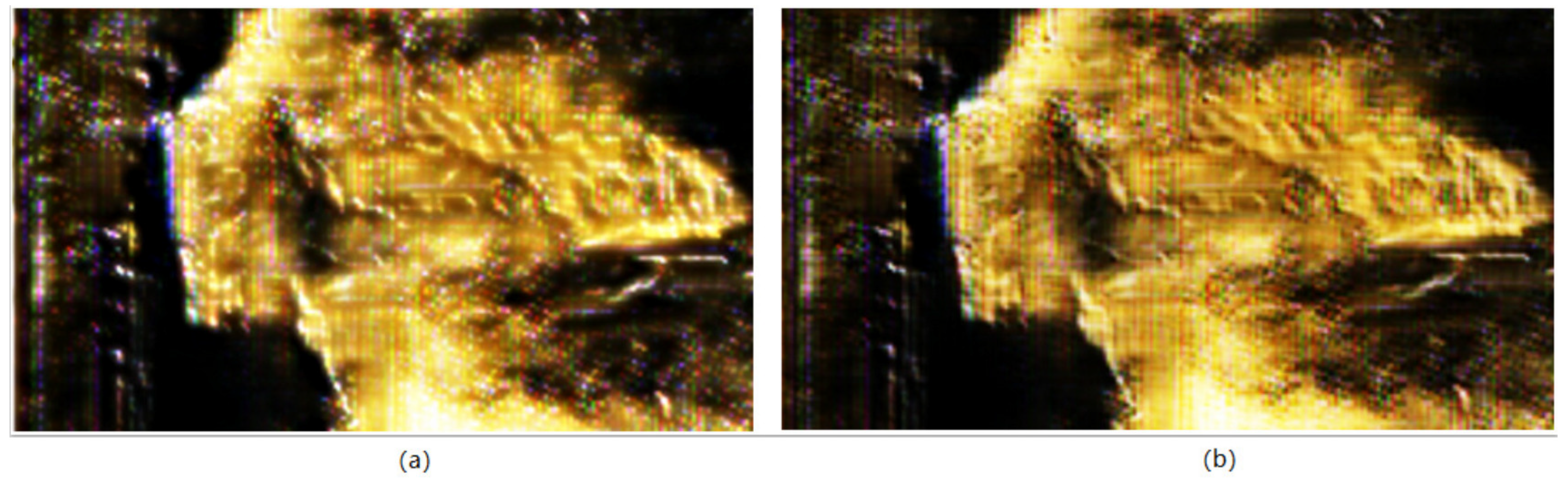
The processed images after applying the Laplacian pyramid and USM (unsharp masking) algorithms are shown in the figure, and significant improvements can be observed compared to the raw generated images. The algorithm mainly optimizes the generated noise (represented as green speckles in the image), enhances texture contrast, and sharpens edge contours. The processed result is shown in
Figure 11.
Subsequent to the generation and post-processing of the images, a computation of pertinent Fréchet inception distance (FID) metrics was conducted. These metrics served to assess the degree of similarity between the generated images and the authentic dataset. Specifically, this assessment involved four distinct comparisons: initially, a comparison between two sets of genuine data, followed by a comparison between entirely unrelated images and the authentic dataset; subsequently, a comparison between the generated data and the authentic dataset; finally, a comparison between the data (subsequent to data enhancement) and the authentic dataset was employed. The outcomes of these comparative analyses are presented in
Table 1.
In this study, an analysis was conducted to compute three distinct metrics, namely the structural similarity index (SSIM), mean squared error (MSE), and mean absolute error (MAE), independently for real images, generated images, and unrelated images. These metrics were separately computed for three pairs: real images compared to real images, real images compared to unrelated images, and real images compared to generated images. The results of these metrics are provided in
Table 2.
Table 1 and
Table 2 reveal that the generated images exhibit FID, MAE, and MSE metrics that are comparable to those of real images, while significantly surpassing the metrics calculated between real images and unrelated images. However, the SSIM metric does not exhibit a similar pattern; in fact, the SSIM metric between the real images and unrelated images is even higher than that between the real images themselves. This phenomenon may be attributed to the lack of structural consistency in the sonar scan results within the experimental region, resulting in pronounced structural disparities among the sonar images.
4.5. Label Generation
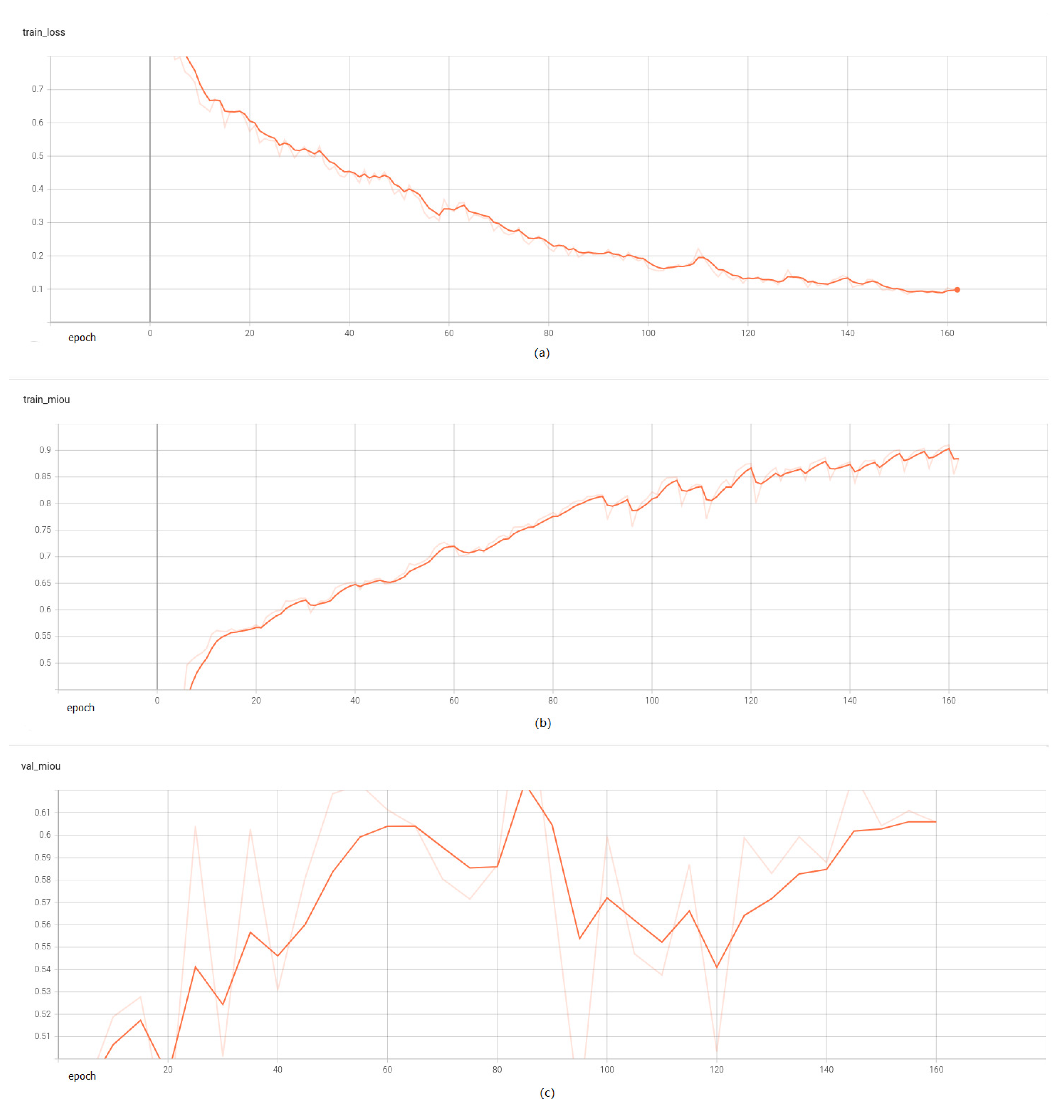
The initial phase involved the training of the semantic segmentation network using authentic data, as depicted in the figure. After 150 episodes, the training process essentially reached convergence, as illustrated in
Figure 12.
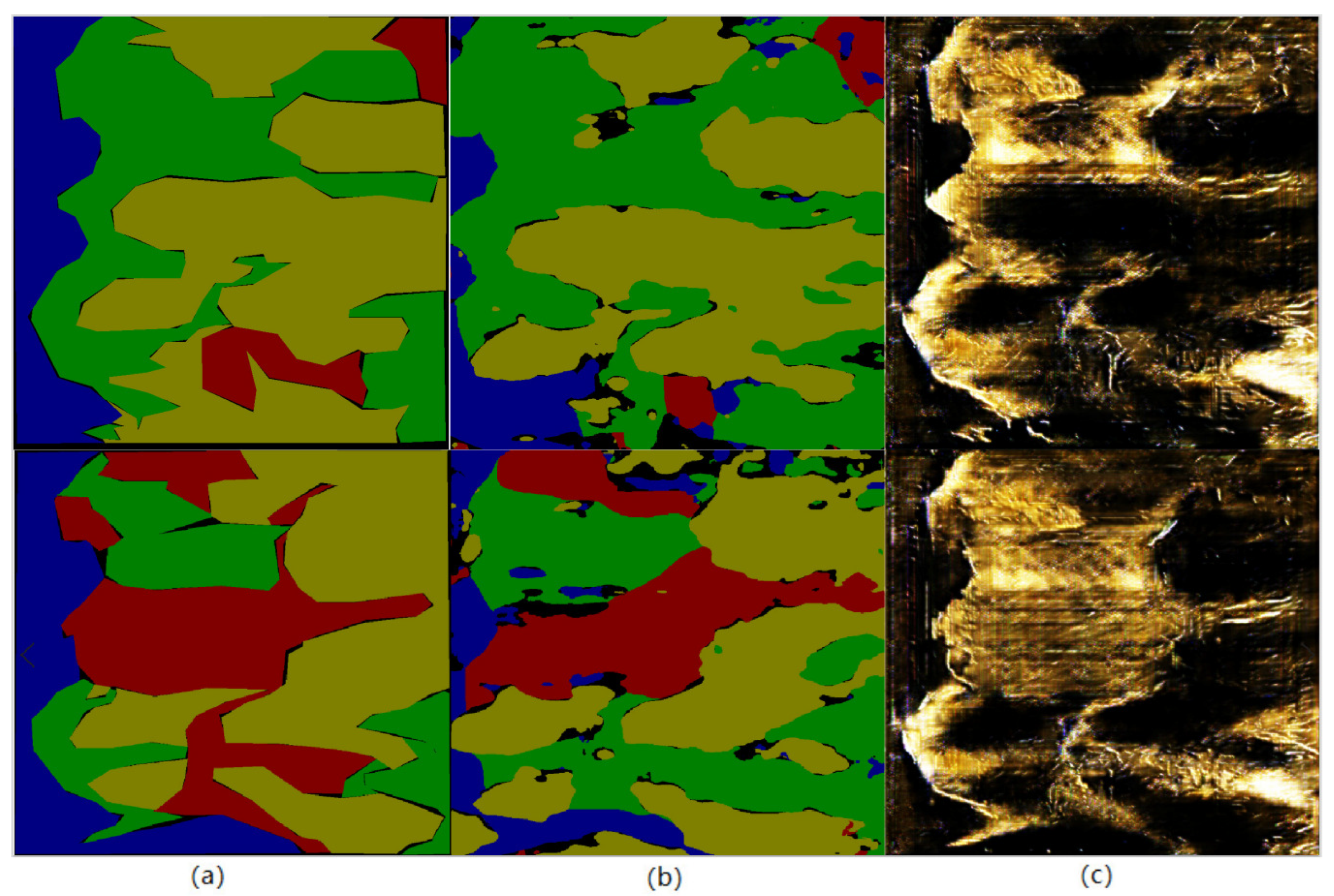
Subsequently, the trained network model was used to autonomously generate labels on the generated images, as shown in the following figure. Blue represents the water body, yellow represents the shaded area, green represents the rock area, red represents the ground area, and black represents the unclassified area. It can be seen that there is still a certain gap between the autonomous labels of the network model and the real ground truth due to the fact that some generated images do not have a water body part, which affects the accuracy of water area division. In terms of image quality, it is still difficult to accurately divide the ground and rock parts. However, the overall effect has been able to reach a usable level after a small amount of manual modification. The results of autonomous labeling are shown in
Figure 13.
Subsequently, a sequence of interconnected experiments was conducted. Initially, the model’s proficiency in semantic segmentation was assessed using authentic data. Subsequently, during the autonomous labeling process of the generated images, the model’s semantic segmentation capabilities for the generated data were examined. Lastly, the manually refined labeled generated data were incorporated into the original authentic dataset to augment the dataset volume. After retraining, an evaluation of the model’s semantic segmentation performance with respect to authentic data was carried out. This comprehensive assessment considered three key evaluation metrics: the mean intersection over union (MIOU), overall accuracy (OA), and F1-score. The outcomes of these assessments are presented in
Table 3.
It can be observed that the second metrics have decreased significantly, indicating a considerable difference in their distributions. However, after minor manual modifications, they can already be utilized as an expanded dataset. Through data augmentation using the generated network, the performance indicators of the semantic segmentation network have improved to some extent (third experiment), demonstrating the usability and effectiveness of the data. It can be seen that the performance indicators of the semantic segmentation network have been improved to a certain extent through the data amplification of the generated network, proving data availability and effectiveness.
5. Conclusions
This article proposes a sidescan sonar image generation model based on a GAN network. This model adopts the design concept of WGAN gp, using trained generators and discriminators to generate and filter data. In response to the noise and clarity issues in the generated images, enhancement algorithms, including the Laplace pyramid and USM algorithm, were used to enhance their signal-to-noise ratio and data adaptability. Through the calculation of metrics such as FID and MSE, it was observed that the generated sonar data closely matched the real data. Furthermore, after undergoing data processing, its level of match was further enhanced. Finally, the designed semantic segmentation model was used to perform preliminary autonomous labeling on the generated data, and the obtained preliminary labels can be put into use after only a rough manual correction. By incorporating the labeled-generated data into the dataset and training the system based on it, it can be observed that the performance of the sidescan sonar semantic segmentation model had improved; the semantic segmentation performance metrics, namely MIOU and F1-score, improved from their original values of 0.677754 and 0.722321 to 0.692736 and 0.723228, respectively. With the inclusion of the augmented sonar data generated, the model’s robustness and generalization capabilities have both shown improvement. In addition, our model also has high portability. Many researchers have proposed large-scale neural network models with poor real-time performance on AUVs. After loading our model into the AUV control terminal, we are still able to complete tasks and have a low dependence on high-performance computers, which is also an important advantage. In the future, we will consider further enhancing the quality of generated sonar data.


