A Deep Reinforcement Learning-Based Path-Following Control Scheme for an Uncertain Under-Actuated Autonomous Marine Vehicle

Abstract

In this article, a deep reinforcement learning-based path-following control scheme is established for an under-actuated autonomous marine vehicle (AMV) in the presence of model uncertainties and unknown marine environment disturbances is presented. By virtue of light-of-sight guidance, a surge-heading joint guidance method is developed within the kinematic level, thereby enabling the AMV to follow the desired path accurately. Within the dynamic level, model uncertainties and time-varying environment disturbances are taken into account, and the reinforcement learning control method using the twin-delay deep deterministic policy gradient (TD3) is developed for the under-actuated vehicle, where path-following actions are generated via the state space and hybrid rewards. Additionally, actor-critic networks are developed using the long-short time memory (LSTM) network, and the vehicle can successfully make a decision by the aid of historical states, thus enhancing the convergence rate of dynamic controllers. Simulation results and comprehensive comparisons on a prototype AMV demonstrate the remarkable effectiveness and superiority of the proposed LSTM-TD3-based path-following control scheme.

1. Introduction

The Autonomous marine vehicle (AMV) is a marine intelligent platform that performs tasks autonomously or semi-autonomously [1], which is widely applied in military and civilian fields due to its small volume, strong concealment, good flexibility and other advantages [2]. In different missions, path following of the AMV plays a crucial role for realized autonomous operation. Considering that, in practice, the AMV inevitably suffers from marine environment disturbances, the path-following control method with high precision and efficiency is crucial to the success of an operation, where a parameterized path is expected to be tracked as accurately as possible [3].

In generally, the path-following control of an AMV consists of two critical parts: kinematics guidance and dynamics control. In the part of guidance research, by calculating the desired heading angle, path-following errors can converge to zero, and in the part of control research, control inputs including surge force and yaw torque are solved using the desired guidance signals, thus contributing to the path following performance [4]. For the former, the light-of-sight (LOS) guidance was widely applied because of its high precision and simplicity [5,6,7,8]. For the latter, fruitful methods were proposed and applied to controller design, such as PID control [9,10], fuzzy control [11,12,13], adaptive control [14,15], active disturbances rejection control [16,17], sliding mode control [18,19], and backstepping control [20,21,22]. In [23], considering the path-following control under unknown environment disturbances, the modified integral LOS guidance law and the adaptive sliding mode control law are developed, realizing the desired path following. In [24], to solve the path-following control of an under-actuated autonomous underwater vehicle subject to environment disturbances, an adaptive robust control method is proposed using fuzzy logic, backstepping and sliding mode technology, where the fuzzy logic system is utilized to approximate the unknown uncertainties. In [25], a novel, adaptive, robust path-following scheme is proposed by combining with the trajectory linearization control and the finite-time disturbance observer. In [26], a fuzzy unknown observer-based, robust, adaptive path-following control scheme is proposed, where the fuzzy observer is designed to estimate lumped unknowns and the observer-based, robust, adaptive tracking control laws are synthesized, thus ensuring that the guided signals are globally asymptotically tracked. However, the above control method depends on a system model with high accuracy, and the derivation process is complex.

With increasingly rapid development of machine learning, deep reinforcement learning (DRL) algorithms are widely applied to the relative studies of unmanned system control [27]. The DRL is a combination of deep learning and reinforcement learning, which has strong decision-making ability and anti-disturbance ability of reinforcement learning and strong representation ability of deep neural network, thus effectively reducing the complexity and difficulty of the controller design. At present, the popular DRL algorithms include the soft actor-critic (SAC), the proximal policy optimization (PPO), and the deep deterministic policy gradient (DDPG) [28,29,30]. In [31], the advantage of actor-critic (A2C) is proposed to solve path-following control for a fish-like robot, where the desired path is a randomly generated curve. In [32], a DRL controller is designed using the DDPG for path following, and simulation shows that the proposed method is better than the PID in terms of transient characteristics. In [33], a distributed DRL method is proposed to solve the path-following control of an under-actuated AMV, where the DDPG-based controller is designed and the radial basis neural network is utilized to approximate the unknown disturbances. In [34], an improved DDPG control method was proposed for path following based on an optimized sampling pool and average motion evaluation network, and the simulation results show that the proposed method effectively improves the utilization rate of samples and avoids falling into a local optimum in the training process. In [35], a linear active disturbances rejection controller based on the SAC was proposed to solve path-following control under wind and wave environments. In [36], the path-following control laws were designed using the twin-delayed deep deterministic policy gradient algorithm (TD3), where desired velocities were generated by the LOS guidance.

Considering the path following of an under-actuated AMV under unknown model parameters and environment disturbances, this article establishes the motion model for an AMV, and proposes a path-following control method by combining with the long short-term memory network (LSTM) and the TD3 algorithm. The main contributions are as follows: (1) within the kinematic level, the surge-heading joint guidance law is developed based on the LOS, where the desired velocity signals are generated to guide the vehicle along the desired path; (2) within the dynamic level, the TD3-based surge-heading controller is developed for the vehicle, where states, actions and reward functions are defined; and (3) to enhance the convergence rate of controller networks, the LSTM layer, using the historical states, is added into the TD3.

The remainder of this article is organized as follows: preliminaries and problem statement are described in Section 2; Section 3 presents the kinematic guidance law and the DRL-based dynamic controller of an AMV; simulation results and analysis are presented in Section 4; and Section 5 contains the conclusion.

2. Preliminaries and Problem Statement

2.1. Reinforcement Learning

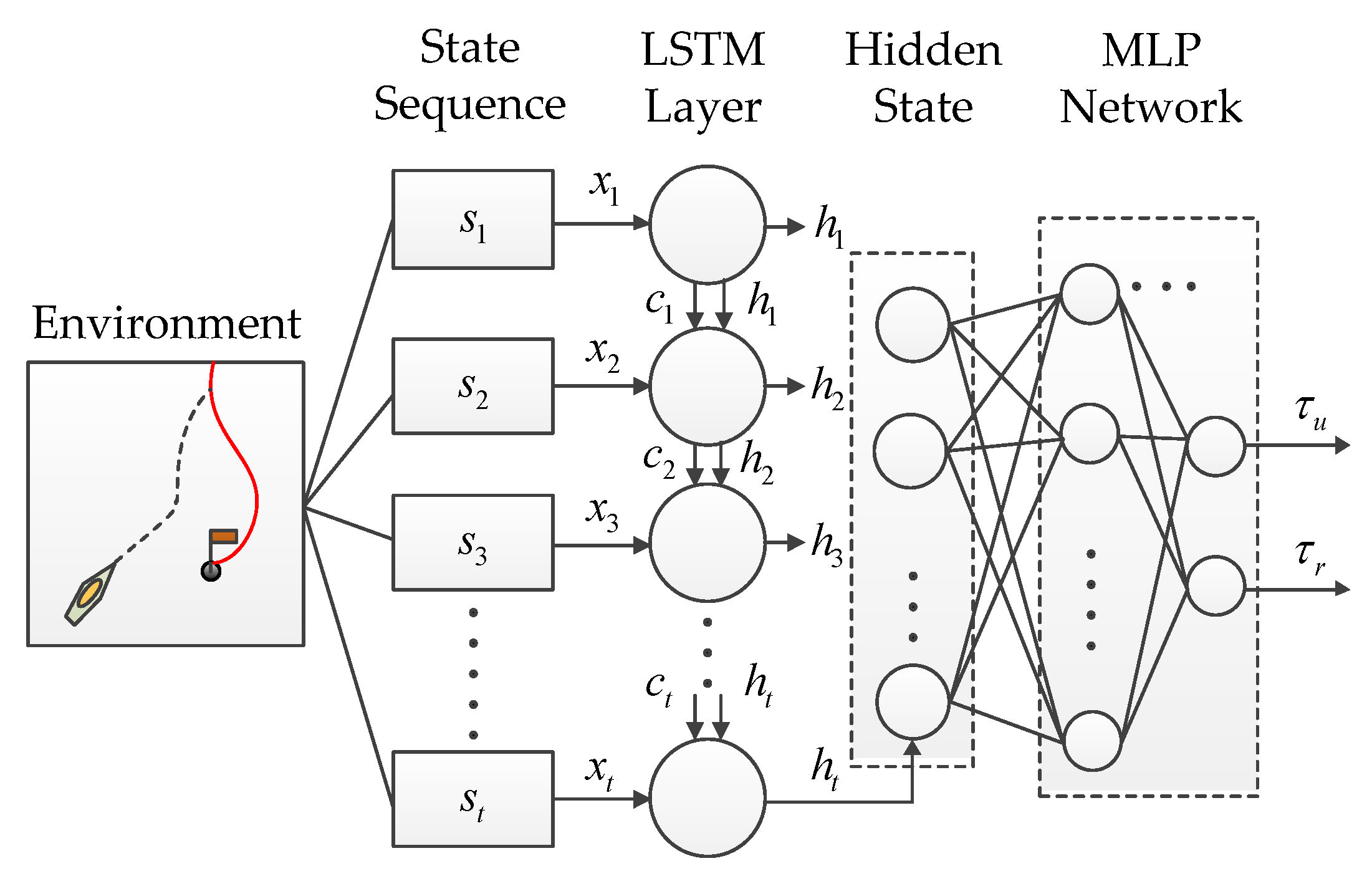
Reinforcement learning is based on the Markov decision process. Four basic elements are defined as $\{S,A,P,R\}$, where $S$ is the set of all states, $A$ is the set of all actions, $P$ is the state transition probability, and $R$ is the reward function [37]. The decay sum of all rewards from a certain state to the final state can be calculated by

$$R_t=r_{t+1}+\gamma r_{t+2}+{\gamma }^2{r}_{t+3}+\dots =\sum _{k=0}^{\infty }{\gamma }^k{r}_{t+k+1}$$

(1)

where $\gamma$ is the discount factor, satisfying $\gamma \in [0,1]$, and $r_{t+i} (i=1,\cdots ,k+1)$ is the reward at the current time.

Additionally, the value functions under the policy $\eta$ include action value function $Q^{\mu }(s_t,a_t)$ and state value function $V^{\mu }(s_t)$, where $s_t$ and $a_t$ are the state and action at the current time. The value functions are described as

$$\left\{\begin{array}{l}{Q}^{\mu }(s_t,a_t)=E_{\mu }[R_t|s_t,a_t]=E_{\mu }[{\displaystyle \sum _{k=0}^{\infty }}{\gamma }^k{r}_{t+k+1}|s_t,a_t]\\ V^{\mu }(s_t)=E_{\mu }[R_t|s_t]=E_{\mu }[{\displaystyle \sum _{k=0}^{\infty }}{\gamma }^k{r}_{t+k+1}|s_t]\end{array}\right.$$

(2)

where $E$ expresses the expectation, and the optimal policy ${\mu }^{\ast }$ can be achieved by maximizing the optimal state-action value functions [38].

$${\mu }^{\ast }=\arg \max V^{\mu }(s_t)=\arg \max Q^{\mu }(s_t,a_t)$$

(3)

2.2. LSTM Network

The LSTM network has better memory ability, where important data is retained and irrelevant noise is deleted, thereby relieving the gradient disappearance of the existing recurrent neural network and the memory burden of networks [39]. The neuronal structure is shown in Figure 1, where $x_t$ is the input; $h_t$ is the output; $c_t$ is the state value of the memory cell at the current time; $h_{t-1}$ and $c_{t-1}$ are the input signals at the previous time; $f_t$ is the forgetting gate; $i_t$ is the input gate; $o_t$ is the output gate; and $\sigma$ is the sigmoid function.

As shown in Figure 1, when the information inputs to the neuron, it firstly goes through the forgetting gate and input gate; then, it goes through the output gate, and the state value of the memory cell $c_t$ are calculated based on the $f_t$ and $i_t$. Finally, the outputs are calculated based on $o_t$ and $c_t$. The renewal process can be described by

$$\left\{\begin{array}{l}{f}_t=\sigma (W_1{x}_t+W_2{h}_{t-1}+b_1)\\ i_t=\sigma (W_3{x}_t+W_4{h}_{t-1}+b_2)\\ o_t=\sigma (W_7{x}_t+W_8{h}_{t-1}+b_4)\\ c_t=c_{t-1}\times f_t+\tanh (W_5{x}_t+W_6{h}_{t-1}+b_3)\times i_t\\ h_t=o_t\times \tanh (c_t)\end{array}\right.$$

(4)

where $W_i$ is the weight coefficient with $i=1,2,\cdots ,8$; $b_h$ is the bias with $h=1,\cdots ,4$, and $\tanh$ is the activation function [40].

2.3. Under-Actuated AMV Model

As described in [41], the under-actuated AMV model of three degrees of freedom in the horizontal plane is written as

$$\left\{\begin{array}{l}\eta =R(\eta )\nu \\ M\dot{\nu }+C(\nu )\nu +D(\nu )\nu ={\tau }_d+\tau \end{array}\right.$$

(5)

where $\eta ={[x,y,\psi ]}^T$ are the positions and heading angle of AMV in the earth-fixed frame, and $\nu ={[u,v,r]}^T$ are the surge, sway and yaw velocities in the body-fixed frame. $\tau ={[{\tau }_u,0,{\tau }_r]}^T$ are the control inputs of path-following, and ${\tau }_d={[{\tau }_{ud},{\tau }_{vd},{\tau }_{rd}]}^T$ are the time-varying marine environment disturbances. $R(\eta )$ is the rotation matrix from the body-fixed frame to the earth-fixed frame, which is defined as

$$R(\eta )=\left[\begin{array}{ccc}\cos \psi & -\sin \psi & 0\\ \sin \psi & \cos \psi & 0\\ 0& 0& 1\end{array}\right]$$

(6)

$M$ is the inertial matrix and satisfies $M=M^T>0$, which is written as

$$M=\left[\begin{array}{ccc}{m}_{11} & 0& 0\\ 0& m_{22}& m_{23}\\ 0& m_{32}& m_{33}\end{array}\right]$$

(7)

$C(\nu )$ is the coriolis-centripetal matrix and satisfies $C(\nu )=-C{(\nu )}^T$, which is written as

$$C(\nu )=\left[\begin{array}{ccc}0& 0& c_{13}(\nu )\\ 0& 0& c_{23}(\nu )\\ -c_{13}(\nu )& -c_{23}(\nu )& 0\end{array}\right]$$

(8)

and $D(\nu )$ is the damping matrix, which is written as

$$D(\nu )=\left[\begin{array}{ccc}{d}_{11}(\nu )& 0& 0\\ 0& d_{22}(\nu )& d_{23}(\nu )\\ 0& d_{32}(\nu )& d_{33}(\nu )\end{array}\right]$$

(9)

with $m_{11}=m-X_{\dot{u}}$, $m_{22}=m-Y_{\dot{v}}$, $m_{33}=I_z-N_{\dot{r}}$, $m_{23}=m{x}_g-Y_{\dot{r}}$, $m_{32}=m{x}_g-N_{\dot{v}}$, $c_{13}(\nu )=-m_{11}v-m_{23}r$, $c_{23}(\nu )=-m_{11}u$, $d_{11}(\nu )=-X_u-X_{|u|u}\left|u\right|-X_{uuu}{\left|u\right|}^2$, $d_{22}(\nu )=-Y_v-Y_{|v|v}\left|v\right|$, $d_{33}(\nu )=-N_r-N_{|v|r}\left|v\right|-N_{|r|r}\left|r\right|$, $Y_{\dot{r}}=N_{\dot{r}}$, where $m$ is AMV mass, and $I_z$ is the moment of inertia in yaw. $X_{*}$, $Y_{*}$ and $N_{*}$ are the hydrodynamic coefficients.

As shown in Figure 2, the desired path $\left(x_d(s), y_d(s)\right)$ is a continuous parameterized curve with a time-independent variable $s$. For any moving point on the curve, a path-tangential angle in the earth-fixed frame is defined as

$$\alpha =atan2\left(y_d^{\prime }(s),x_d^{\prime }(s)\right)$$

(10)

where $y_d^{\prime }(s)=\partial y_d/\partial s$, $x_d^{\prime }(s)=\partial x_d/\partial s$. The errors between $\left(x, y\right)$ and $\left(x_d, y_d\right)$ can be formulated as

$$\left[\begin{array}{l}{x}_e\\ y_e\end{array}\right]={\left[\begin{array}{l}\cos \alpha -\sin \alpha \\ \sin \alpha \cos \alpha \end{array}\right]}^T\left[\begin{array}{l}x-x_d(s) \\ y-y_d(s) \end{array}\right]$$

(11)

where $x_e$ is the along-track error, and $y_e$ is the cross-track error.

In this article, our objective is to design the DRL-based path-following control scheme for an uncertain under-actuated AMV, such that the vehicle can follow the desired path with the desired velocities regardless of model uncertainties and unknown marine environment disturbances. To be specific, the objective can be formalized as

$$\left\{\begin{array}{l}\underset{t\to \infty }{\lim }{x}_e\le {\delta }_x\\ \underset{t\to \infty }{\lim }{y}_e\le {\delta }_y\end{array}\right.$$

(12)

where ${\delta }_x$ and ${\delta }_y$ are any small positive constants.

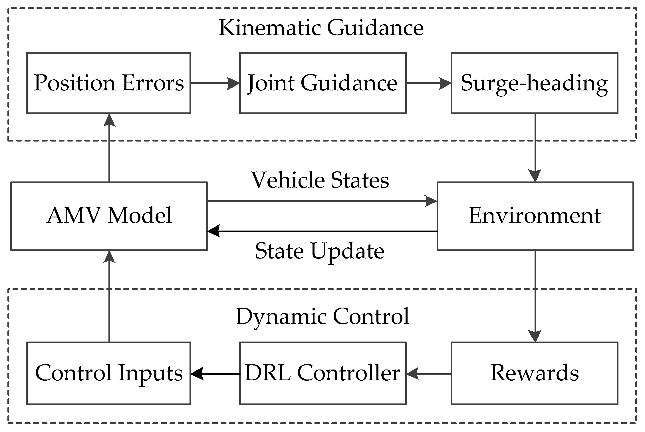
3. DRL-Based Path-Following Control Scheme

In this section, a DRL-based path-following control scheme is established for an under-actuated AMV in the presence of model uncertainties and unknown marine environment disturbances. The diagram of the proposed control scheme is shown in Figure 3, where kinematic guidance and dynamic control are designed, respectively.

Within the kinematic level, according to the position errors and related motion states obtained by the AMV model, the desired surge velocity and heading angle are generated by the designed surge-heading joint guidance law based on the light-of-sight guidance. Within the dynamic level, DRL-based surge-heading controllers are presented for following the desired guidance signals. The reward function is designed to generate rewards by comparing the desired signals with the actual vehicle states in the environment. The controllers generate the control inputs based on the rewards, and the vehicle precisely tracks the desired signals based on the control inputs and the novel environment states to realize path-following control. By combining with the kinematic guidance and dynamic control, the objective (12) can be successfully completed.

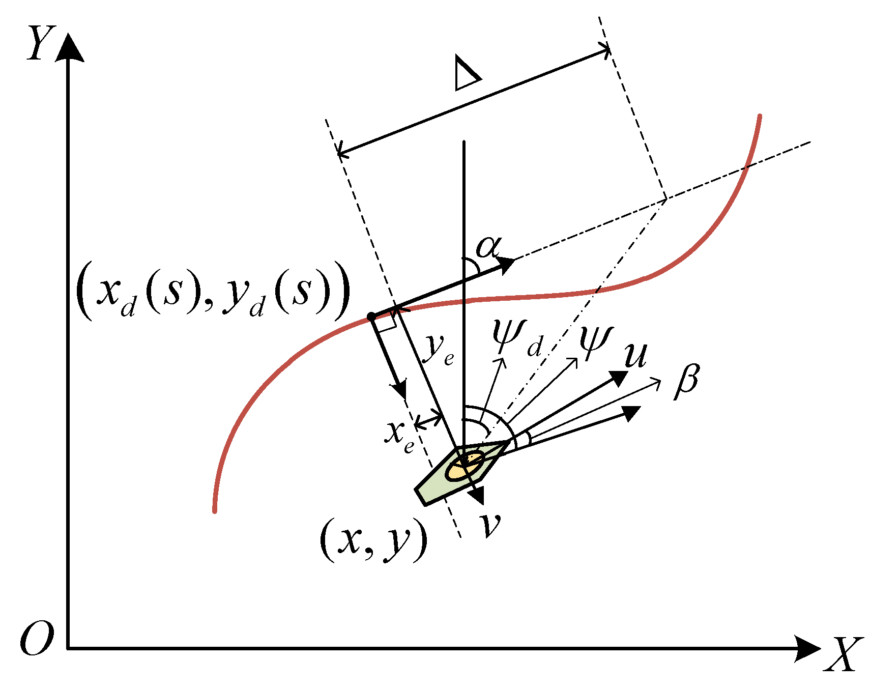
3.1. Kinematic Guidance Design

Firstly, kinematic guidance is designed in this subsection, where desired surge velocities and heading angles are produced. Differentiating (11) along (5) yields

$$\left\{\begin{array}{l}{\dot{x}}_e=u\cos \left(\psi -\alpha \right)-v\sin \left(\psi -\alpha \right)+\dot{\alpha }{y}_e-u_s\\ {\dot{y}}_e=u\sin \left(\psi -\alpha \right)+v\cos \left(\psi -\alpha \right)-\dot{\alpha }{x}_e\end{array}\right.$$

(13)

where $u_s$ is velocity of the virtual point along the desired path, which is defined by

$$u_s=\dot{s}\sqrt{{x_d^{\prime }}^2(s)+{y_d^{\prime }}^2(s)}$$

(14)

Define the sideslip angle of under-actuated vehicle as

$$\beta =\arctan \left(\frac{v}{u}\right)$$

(15)

In this context, path-following error dynamics (13) is rewritten as

$$\left\{\begin{array}{l}{\dot{x}}_e=u\cos \left(\psi -\alpha \right)-u\sin \left(\psi -\alpha \right)tan\beta +\dot{\alpha }{y}_e-u_s\\ {\dot{y}}_e=u\sin \left(\psi -\alpha \right)+u\cos \left(\psi -\alpha \right)tan\beta -\dot{\alpha }{x}_e\end{array}\right.$$

(16)

Then, select the Lyapunov function related to path following errors as

$$V=\frac{1}{2}\left(x_e^2+y_e^2\right)$$

(17)

The time derivative of (17) along the solution (16) is

$$\begin{array}{l}\dot{V}=x_e{\dot{x}}_e+y_e{\dot{y}}_e\\ \hspace{1em}=x_e\left(u\cos (\psi -\alpha )-u\sin (\psi -\alpha )tan\beta \left.+\dot{\alpha }{y}_e-u_s\right)\right.\\ \hspace{1em}+y_e\left(u\sin (\psi -\alpha )-\dot{\alpha }{x}_e\left.+u\cos (\psi -\alpha )tan\beta \right)\right.\end{array}$$

(18)

Thus, the surge-heading joint guidance law is designed as follows

$$\left\{\begin{array}{l}{u}_d=k_1\sqrt{y_e^2+{\Delta }^2}\\ {\psi }_d=\alpha -{\beta }_d-\arctan \left(\frac{y_e}{\Delta }\right)\end{array}\right.$$

(19)

where $k_1>0$; $\Delta >0$ is the look-ahead distance; ${\beta }_d=\arctan \left(v/u_d\right)$ and virtual velocity $u_s$ is determined by

$$u_s=U_d\cos \left({\beta }_d+\psi -\alpha \right)+k_2{x}_e$$

(20)

with $k_2>0$ and $U_d=\sqrt{u_d^2+v^2}$.

Using the fact

$$\left\{\begin{array}{l}\sin \left({\tan }^{-1}\left(-\frac{y_e}{\Delta }\right)\right)=-\frac{y_e}{{\left(y_e^2+{\Delta }^2\right)}^{1/2}}\\ \cos \left({\tan }^{-1}\left(-\frac{y_e}{\Delta }\right)\right)=-\frac{\Delta }{{\left(y_e^2+{\Delta }^2\right)}^{1/2}}\end{array}\right.$$

(21)

and substituting the guidance law (19) into (18) yield

$$\begin{array}{l}\dot{V}=x_e\left(\dot{\alpha }{y}_e-k_2{x}_e\right)+y_e\left(-\frac{k_1}{\cos {\beta }_d}{y}_e-\dot{\alpha }{x}_e\right)\\ \hspace{1em}=-k_2{x}_e^2-\frac{k_1}{\cos {\beta }_d}{y}_e^2\end{array}$$

(22)

Since $0<\cos {\beta }_d\le 1$ renders $\dot{V}\le -k_2{x}_e^2-k_1{y}_e^2$, it indicates that path-following error $x_e$ and $y_e$ can globally asymptotically converge to the origin using the proposed guidance method.

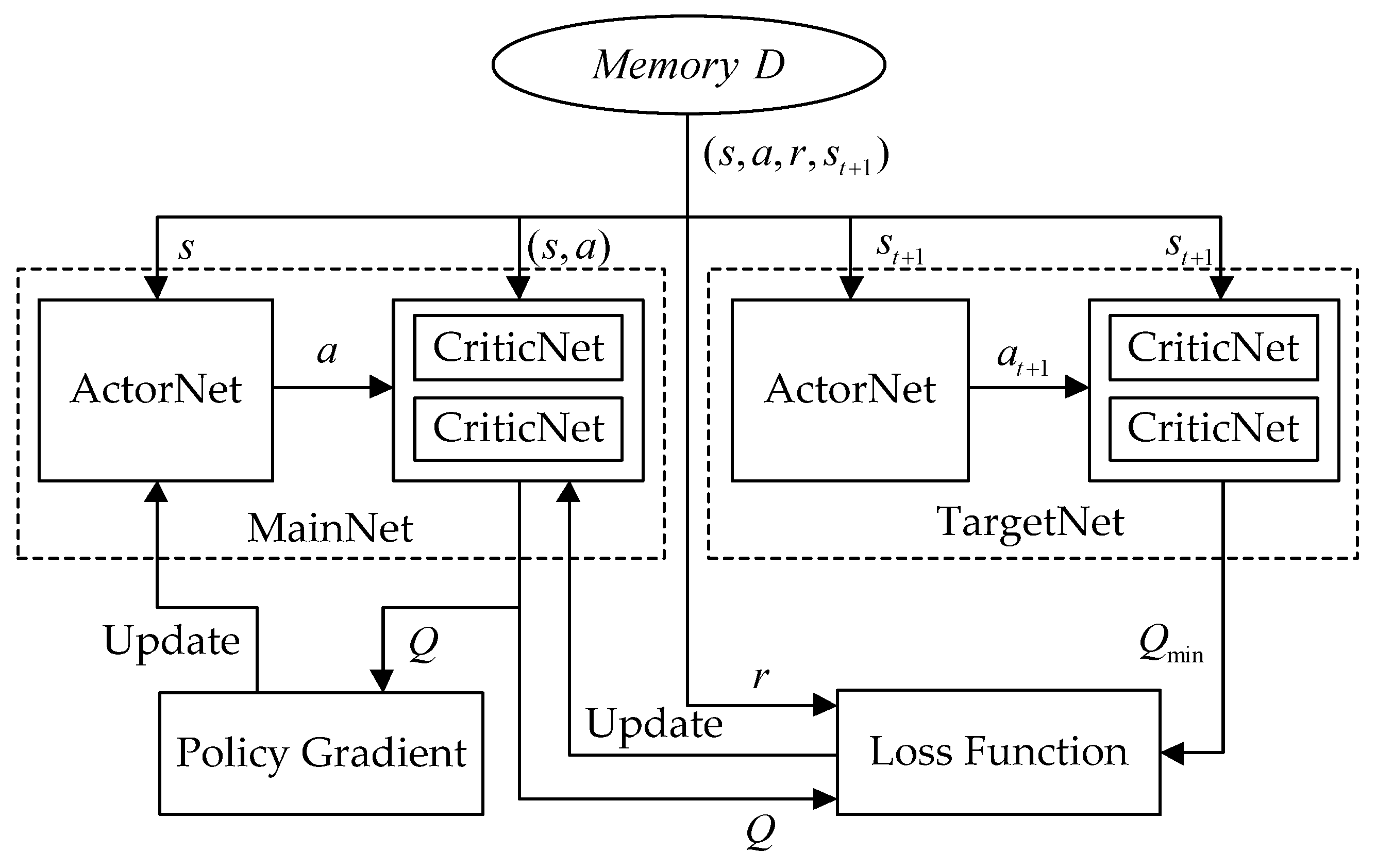
3.2. Dynamic Control Design

Because of inaccurate measurements and environment disturbances, AMV model parameters cannot be obtained completely, thereby resulting in uncertainties of dynamics. To enhance the engineering practicality and reduce the complexity of controllers, a TD3-based reinforcement learning control method is presented within the dynamic level, where control inputs of the AMV are generated successfully.

The main purpose of the DRL algorithm is to make the vehicle take actions in the case of different path information. The proposed TD3 algorithm is based on the actor-critic structure, where policy functions are produced using actor networks and critic networks used to judge the performance of the actor [42]. Additionally, LSTM network layers are introduced into the TD3 and thereby enhance the utilization rate of historical states.

Firstly, the network structure of TD3 algorithm is shown in Figure 4. By virtue of initial environment states, actions of the AMV are generated using actor networks, and rewards are accordingly calculated using reward functions; thus, the states can be updated with the generated actions. The empirical value is defined as $e(t)=\{s,a,r,s_{t+1}\}$ and saved into buffer $MemoryD$. Through repeated training, the empirical replay sequence $D=\{e_1,e_2,\dots ,e_n\}$ can be formed. Considering that the adjacent actions of path-following have strong relevance, a batch of empirical sequences are selected randomly for training. The actor network of target generates the action $a_{t+1}$ according to the state $s_{t+1}$ in the empirical replay sequence, and the critic network of target calculates the $Q_{\min }$ value, where $Q_{\min }$ is the smaller of the two $Q_{target}$ values generated by target networks. Two critic networks are updated based on $Q$, $Q_{\min }$ and loss functions. Actor networks generate actions using states. Critic networks generate the $Q$ value using states and actions, and thus calculate the policy gradient and update actor networks using the $Q$ value.

The specific renewal process is as follows. Considering that TD3 algorithm is a deterministic policy and has the characteristic of target policy smoothing regularization, random noise $\epsilon$ is added into target actions. Therefore, there is $a_{t+1}={\mu }^{\prime }(s_{t+1}|w^{\prime })+\epsilon$, where ${\mu }^{\prime }$ is the policy of target actor networks, and $w^{\prime }$ is the parameter of target actor networks.

The target value is calculated as

$$y=r+\gamma Q_{\min }(s_{t+1},a_{t+1}|{\theta }_i^{\prime })$$

(23)

where $i=1, 2$, ${\theta }_i^{\prime }$ represents parameters of target critic networks.

The loss function is defined as

$$L({\theta }_i)=\frac{1}{N}{\left(y-Q(s,a|{\theta }_i)\right)}^2$$

(24)

where $N$ represents the number of mini-batch, and ${\theta }_i$ represents parameters of critic networks. The gradient is updated by

$$\frac{\partial L({\theta }_i)}{\partial {\theta }_i}=E\left[\left(y-Q(s,a|{\theta }_i)\right)\frac{\partial Q(s,a|{\theta }_i)}{\partial {\theta }_i}\right]$$

(25)

Subsequently, the policy gradient of actor networks is updated by

$$\left\{\begin{array}{l}\frac{\partial J(w)}{\partial w}=E\left[\frac{\partial Q(s,a|\theta )}{\partial a}\frac{\partial \mu (s|w)}{\partial w}\right]\\ {\nabla }_{w}J\approx \frac{1}{N}\sum ({\nabla }_{\mathrm{a}}Q(s,a|{\theta }_1){|}_{a=\mu (s)}{\nabla }_w\mu (s|w))\end{array}\right.$$

(26)

After a couple of cycles, target parameters are soft updated by

$$\left\{\begin{array}{l}{\theta }_i^{\prime }=\xi {\theta }_i+\left(1-\xi \right){\theta }_i^{\prime }\\ w^{\prime }=\xi w+\left(1-\xi \right)w^{\prime }\end{array}\right.$$

(27)

where $\xi \in \left(0,1\right)$ represents the learning rate.

Then, the LSTM network is introduced into actor-critic networks, thus contributing to the LSTM-TD3-based reinforcement learning controllers. The LSTM-TD3 network still retains the actor-critic structure, where LSTM inputs is a length of sequences. According to the real-time navigational information, the continuous states are saved into the sequences. The LSTM network layer is connected to generate the final hidden state $h_t$, where $h_t$ is a one-dimensional array. Via the multi-layer perceptron (MLP) neural networks, the path-following control inputs of an AMV are generated, which include surge forces and yaw torques. The network structure of the actor is shown in Figure 5. Note that the critic has the similar network structure to the actor, and generates available actions.

Finally, the state space, action space and reward function are designed as follows. To be specific, the state space represents perceived environment information of the AMV, which is the basis of decision-making and reward-evaluating. The action space represents control inputs of the AMV, including surge forces and yaw torques. The reward function is used to evaluate current state of the AMV.

In this context, the state space is defined as

$$s_t=[x_e, y_e, \psi , {\psi }_e, u, v, r, u_e, {\tau }_{u(}{}_{t-1)}, {\tau }_{r(}{}_{t-1)}]$$

(28)

where ${\tau }_{u(}{}_{t-1)}$ and ${\tau }_{r(}{}_{t-1)}$ are control inputs at the previous moment. $u_e=u-u_d$ and ${\psi }_e=\psi -{\psi }_d$ with $u_d$, ${\psi }_d$ are generated by the guidance law (19).

Taking path-following errors, surge velocity and heading angle errors into considerations, the reward function $r_1$ is designed as

$$r_1=\lambda \left(2{\exp }^{-k_3|u_e|}-1\right)+\left(2{\exp }^{-k_4|{\psi }_e|}-1\right)+\left(2{\exp }^{-k_5|\sqrt{x_e^2+y_e^2}|}-1\right)$$

(29)

where $k_{\ast }(\ast =3,4,5)>0$ and $\lambda >0$. Note that the exponential function is used to calculate rewards, which limits the size of rewards and avoids high rewards.

Furthermore, the reward function $r_2$ is designed as

$$r_2={\exp }^{-k_6|{\sigma }_{{\tau }_u}|}+{\exp }^{-k_6|{\sigma }_{{\tau }_r}|}-1$$

(30)

where $k_6>0$; ${\sigma }_{{\tau }_u}$ and ${\sigma }_{{\tau }_r}$ are the standard deviation of two inputs, which are used to reduce the chattering of control inputs.

By combining with (29) and (30), the hybrid rewards of path-following control are established as

$$r=r_1+k_7{r}_2$$

(31)

where $k_7>0$, and satisfies $k_7\in (0,1)$.

The framework of the dynamic control algorithm is summarized in Algorithm 1.

Algorithm 1. Dynamic control algorithm of an AMV.

Inputs: Learning rate $\xi$, $l_{\theta }$ and $l_w$, regular factor $\epsilon$, gradient threshold parameter $g$, discount factor $\gamma$, sequence length $L$, the maximum number of steps per training $K$, updating cycle of target network parameter $d$, training cycle $F$, mini-batch $N$.

Initialize: Critic network $Q(s,a|{\theta }_i)$ and actor network $\mu (s|w)$ with random parameters ${\theta }_1$, ${\theta }_2$ and $w$, target network ${\theta }_1^{\prime }\leftarrow {\theta }_1$, ${\theta }_2^{\prime }\leftarrow {\theta }_2$ and $w^{\prime }\leftarrow w$, experience replay buffer $Memory D$, navigation environment of an AMV.

Procedure: 1: for  $n_1=1,\dots ,F$ do 2:   for  $n_2=1,\dots ,K$ do

3:   Select actions with exploration noise $a~\mu (s|w)+\epsilon$ and obtain reward $r$ and next moment state $s_{t+1}$

4:   Save transition tuple $(s,a,r,s_{t+1})$ into $Memory D$ 5:   Sample $N$ transitions $(s,a,r,s_{t+1})$ $\left\{\begin{array}{l}{a}_{t+1}\leftarrow {\mu }^{\prime }(s_{t+1}|w^{\prime })+\epsilon \\ y\leftarrow r+\gamma Q_{\min }(s_{t+1},a_{t+1}|{\theta }_i^{\prime })\end{array}\right.$ 6:   Update Critic networks parameters ${\theta }_i$ as ${\theta }_i\leftarrow \arg {\min }_{{\theta }_i}\frac{1}{N}{\left(y-Q(s,a|{\theta }_i)\right)}^2$ 7:   if $t$ mod $d$ then

8:    Update actor network parameters $w$ as ${\nabla }_{w}J\approx \frac{1}{N}\sum ({\nabla }_{\mathrm{a}}Q(s,a|{\theta }_1){|}_{a=\mu (s)}{\nabla }_w\mu (s|w))$

9:    Update target network as $\left\{\begin{array}{l}{\theta }_i^{\prime }=\xi {\theta }_i+\left(1-\xi \right){\theta }_i^{\prime }\\ w^{\prime }=\xi w+\left(1-\xi \right)w^{\prime }\end{array}\right.$ end if  end for

Outputs: Actor network parameter $w$, critic network parameters ${\theta }_1$ and ${\theta }_2$.

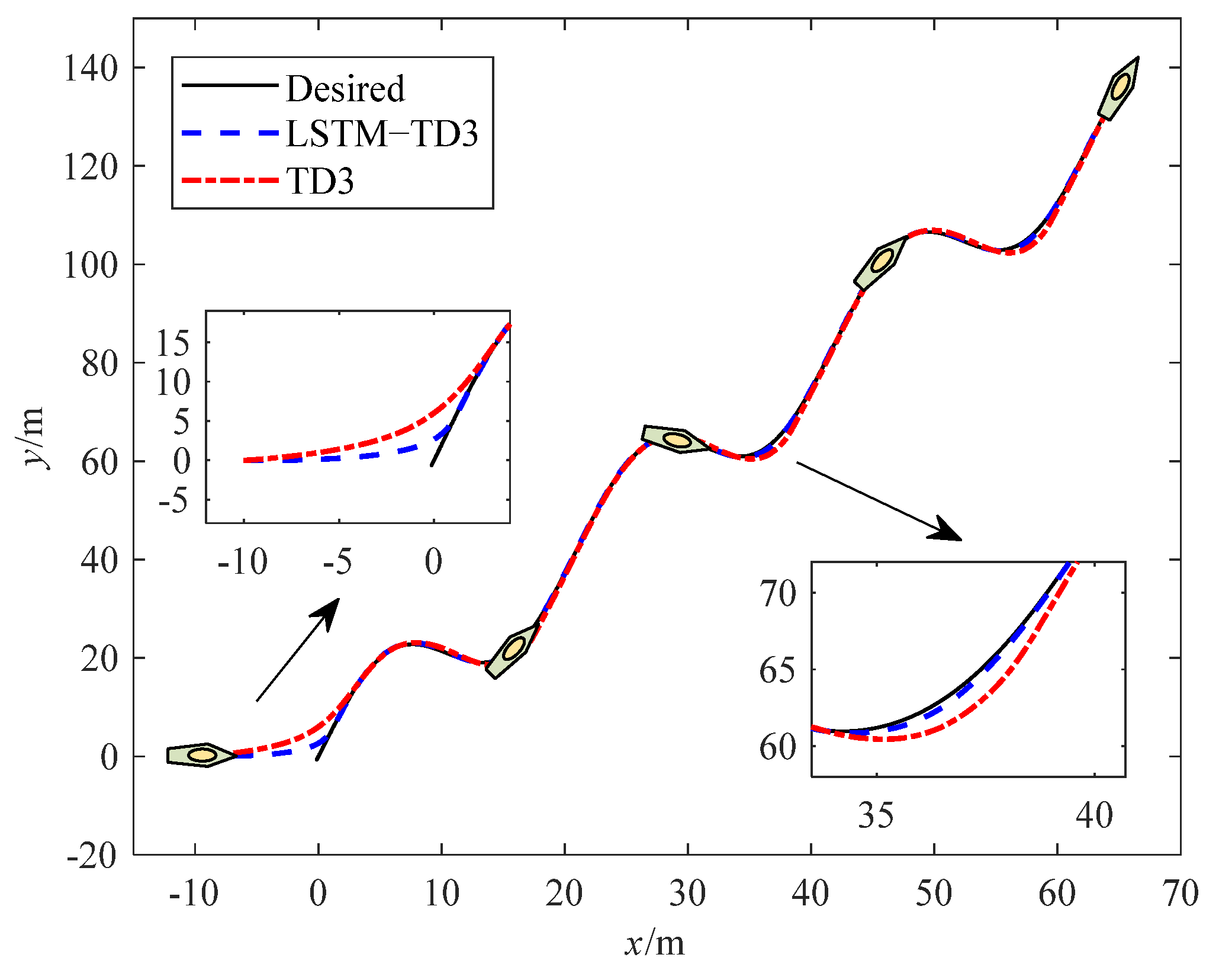
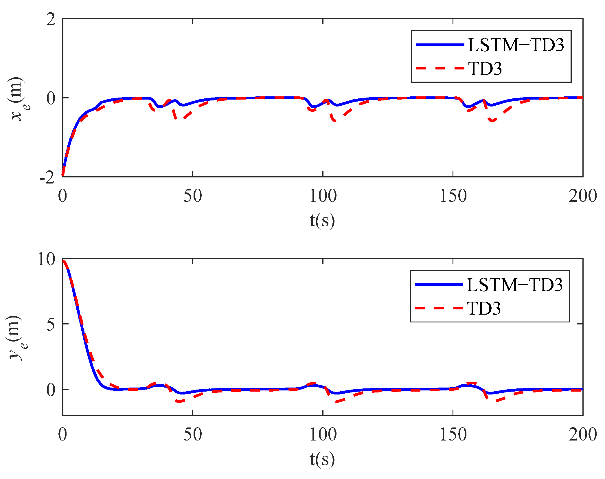
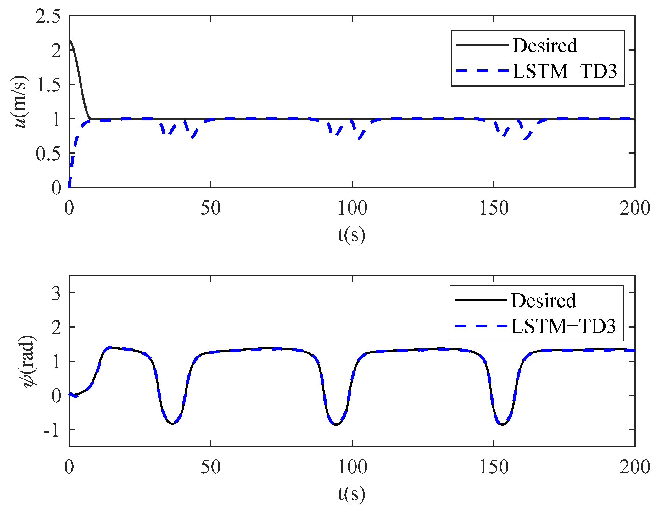
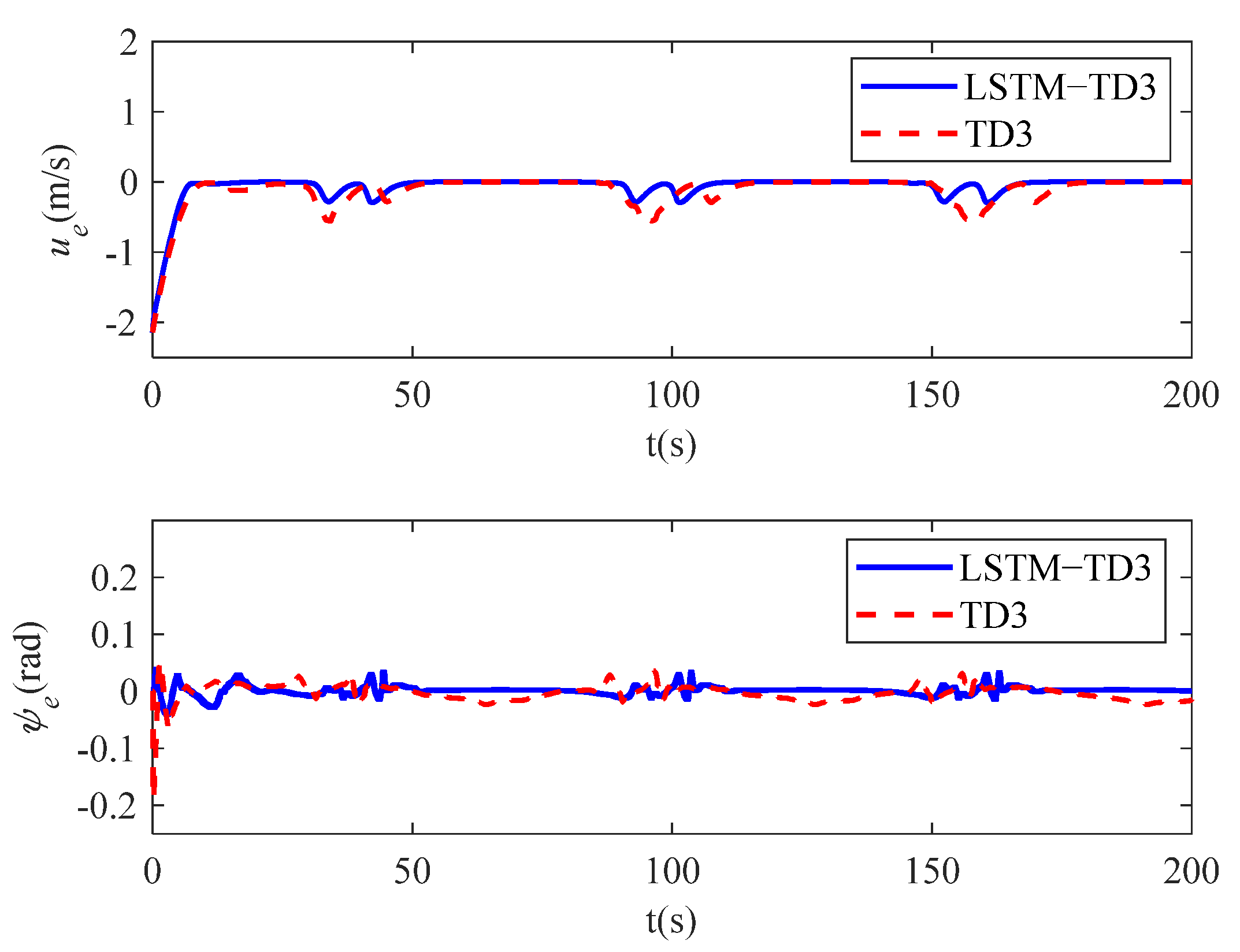
4. Simulation Studies

In this section, simulation studies are shown to verify the effectiveness and superiority of the proposed DRL-based path-following control method. Consider an under-actuated AMV described by (5) with model uncertainties and unknown marine environment disturbances. Model parameters of the prototype AMV can be found in [43].

Within the kinematic guidance level, relative parameters are chosen as follows: $k_1=0.2$, $k_2=2$, $\Delta =3$. Within the dynamic control level, relative parameters are chosen as follows: $k_3=1.5$, $k_4=6$, $k_5=1$, $k_6=1$, $\lambda =0.8$, $k_7=0.3$. Training hyper parameters and network parameters of the LSTM-TD3 are shown in

Table 1. Training hyper parameters.

Parameters	Value
Discount factor $\gamma$	0.99
State sequence length $L$	20
Training cycle $F$	1000
Maximum number of steps $K$	1000
Capacity of buffer $D$	100,000
Learning rate $l$	0.001
Optimizer	Adam
Gradient threshold parameter $g$	1
Regular factor $\epsilon$	0.00005
Mini-batch $N$	128

and

Table 2. LSTM-TD3 network parameters.

Parameters	Value
Input layer of actor network	11
Input layer of critic network	13
Fully connected layer	200
LSTM layer of actor network	100
LSTM layer of critic network	100
Output layer of actor	2
Output layer of critic	1

, respectively.

Episode rewards with different DRL algorithms of path-following control of an AMV are shown in Figure 6. It can be seen that the initial reward is extremely low since the vehicle explores the environment randomly during the initial training stage. After collecting enough data, the rewards converge to a stable value under the DRL control method. Compared to the asynchronous advantage of actor-critic (A3C) developed in [44], the TD3 and LSTM-TD3 can effectively increase the accumulated reward. Additionally, the proposed LSTM-TD3 shows a faster convergence rate and a more stable convergence process than the other two algorithms.

After training the algorithm for 1000 episodes, the optimal actor network parameters of the LSTM-TD3 and TD3 are saved and utilized. Simulation time is set as 200s. The initial positions and attitude are $\eta ={[-10,0,0]}^T$ and the initial velocities are $\nu ={[0,0,0]}^T$. Time-varying marine environment disturbances are defined as

$${\tau }_d=\left[\begin{array}{c}5\sin \left(0.1t+\pi /5\right)\\ 2.2\cos \left(0.1t+6\right)\\ 1.2\cos \left(0.1t+3\right)\end{array}\right]$$

(32)

The desired path is defined as

$$\left\{\begin{array}{l}{x}_d=s\\ y_d=10\sin (0.3s)+2s\end{array}\right.$$

(33)

Simulation results are shown in Figure 7, Figure 8, Figure 9, Figure 10 and Figure 11. Figure 7 shows the path-following control performance of an under-actuated AMV where the desired path, actual path under the proposed LSTM-TD3 and the traditional TD3 are plotted. Obviously, the proposed control method has significant superiority in terms of transient responses and steady-state performance. Figure 8 shows the path-following errors of an AMV subject to model uncertainties and marine environment disturbances. It can be seen that the tangential error and the normal error can converge to the origin faster under the proposed control method. Figure 9 shows the surge velocity and heading angle, where desired signals are generated by guidance law (19). The actual velocities gradually converge to the desired value by the aid of the DRL controller. Note that the slight chattering of velocities is due to large path inflection point, and under-actuated AMV have to reduce their speed to follow the desired path. Figure 10 shows the velocity error and heading angle error of an AMV. It can be seen that the LSTM network considers historical states and thus enhances control performance. Figure 11 shows path-following control inputs of an AMV, including the surge force and the yaw torque. Because of the hybrid rewards with standard deviation, where 20 continuous inputs are set as a calculation group and dynamic sliding is introduced, the control chattering is effectively relieved.

5. Conclusions

This article studies the path-following control of an under-actuated AMV subject to unknown model parameters and marine environmental disturbances. Within the kinematic level, a surge-heading joint guidance law is presented, and makes the vehicle follow the desired path. Within the dynamic level, a LSTM-TD3-based reinforcement learning controller is presented, where vehicle actions are generated by the state space and hybrid reward. Additionally, actor-critic networks are developed using the LSTM network, and vehicles can make a decision by the aid of historical states, thus enhancing the convergence rate of controller networks. Simulation results and comprehensive comparisons demonstrate the remarkable effectiveness and superiority of the proposed path-following control method. By the aid of the proposed controller, the AMV can achieve path following regardless of marine environment disturbances.

References

1. Jorge, V.A.; Granada, R.; Maidana, R.G.; Jurak, D.A.; Heck, G.; Negreiros, A.P.; Dos Santos, D.H.; Gonçalves, L.M.; Amory, A.M. A Survey on Unmanned Surface Vehicles for Disaster Robotics: Main Challenges and Directions. Sensors 2019, 19, 702. [Google Scholar] [CrossRef]
2. Liu, T.; Dong, Z.; Du, H.; Song, L.; Mao, Y. Path Following Control of the Underactuated USV Based on the Improved Line-of-Sight Guidance Algorithm. Pol. Marit. Res. 2017, 24, 3–11. [Google Scholar] [CrossRef]
3. Mu, D.; Wang, G.; Fan, Y.; Bai, Y.; Zhao, Y. Fuzzy-Based Optimal Adaptive Line-of-Sight Path Following for underactuated unmanned surface vehicle with uncertainties and time-varying disturbances. Math. Probl. Eng. 2018, 2018, 7512606. [Google Scholar] [CrossRef]
4. Koh, S.; Zhou, B.; Fang, H.; Yang, P.; Yang, Z.; Yang, Q.; Guan, L.; Ji, Z. Real-time deep reinforcement learning based vehicle navigation. Appl. Soft Comput. 2020, 96, 106694. [Google Scholar] [CrossRef]
5. Mu, D.; Wang, G.; Fan, Y.; Bai, Y.; Zhao, Y. Path following for podded propulsion unmanned surface vehicle: Theory, simulation and experiment. IEEJ Trans. Electr. Electron. Eng. 2018, 13, 911–923. [Google Scholar] [CrossRef]
6. Lekkas, A.M.; Fossen, T.I. Integral LOS Path Following for Curved Paths Based on a Monotone Cubic Hermite Spline Parametrization. IEEE Trans. Control Syst. Technol. 2014, 22, 2287–2301. [Google Scholar] [CrossRef]
7. Fossen, T.I.; Lekkas, A.M. Direct and indirect adaptive integral line-of-sight path-following controllers for marine craft exposed to ocean currents. Int. J. Adapt. Control Signal Process. 2017, 31, 445–463. [Google Scholar] [CrossRef]
8. Fossen, T.I.; Pettersen, K.Y.; Galeazzi, R. Line-of-Sight Path Following for Dubins Paths with Adaptive Sideslip Compensation of Drift Forces. IEEE Trans. Control Syst. Technol. 2014, 23, 820–827. [Google Scholar] [CrossRef]
9. Liu, Z.; Song, S.; Yuan, S.; Ma, Y.; Yao, Z. ALOS-Based USV Path-Following Control with Obstacle Avoidance Strategy. J. Mar. Sci. Eng. 2022, 10, 1203. [Google Scholar] [CrossRef]
10. Rout, R.; Subudhi, B. Inverse optimal self-tuning PID control design for an autonomous underwater vehicle. Int. J. Syst. Sci. 2017, 48, 367–375. [Google Scholar] [CrossRef]
11. Yu, C.; Xiang, X.; Lapierre, L.; Zhang, Q. Nonlinear guidance and fuzzy control for three-dimensional path following of an underactuated autonomous underwater vehicle. Ocean Eng. 2017, 146, 457–467. [Google Scholar] [CrossRef]
12. Xiang, X.; Yu, C.; Zhang, Q. Robust fuzzy 3D path following for autonomous underwater vehicle subject to uncertainties. Comput. Oper. Res. 2017, 84, 165–177. [Google Scholar] [CrossRef]
13. Zhang, J.; Xiang, X.; Lapierre, L.; Zhang, Q.; Li, W. Approach-angle-based three-dimensional indirect adaptive fuzzy path following of under-actuated AUV with input saturation. Appl. Ocean Res. 2021, 107, 102486. [Google Scholar] [CrossRef]
14. Sahu, B.K.; Subudhi, B. Adaptive tracking control of an autonomous underwater vehicle. Int. J. Autom. Comput. 2014, 11, 299–307. [Google Scholar] [CrossRef]
15. Shin, J.; Kwak, D.J.; Lee, Y. Adaptive Path-Following Control for an Unmanned Surface Vessel Using an Identified Dynamic Model. IEEE/ASME Trans. Mechatron. 2017, 22, 1143–1153. [Google Scholar] [CrossRef]
16. Lamraoui, H.C.; Zhu, Q. Path following control of fully-actuated autonomous underwater vehicle in presence of fast-varying disturbances. Appl. Ocean Res. 2019, 86, 40–46. [Google Scholar] [CrossRef]
17. Zhang, H.; Zhang, X.; Cao, T.; Bu, R. Active disturbance rejection control for ship path following with Euler method. Ocean Eng. 2022, 247, 110516. [Google Scholar] [CrossRef]
18. Zhang, G.; Huang, H.; Wan, L.; Li, Y.; Cao, J.; Su, Y. A novel adaptive second order sliding mode path following control for a portable AUV. Ocean Eng. 2018, 151, 82–92. [Google Scholar] [CrossRef]
19. Zhang, H.; Zhang, X.; Bu, R. Radial Basis Function Neural Network Sliding Mode Control for Ship Path Following Based on Position Prediction. J. Mar. Sci. Eng. 2021, 9, 1055. [Google Scholar] [CrossRef]
20. Wang, J.; Wang, C.; Wei, Y.; Zhang, C. Three-Dimensional Path Following of an Underactuated AUV Based on Neuro-Adaptive Command Filtered Backstepping Control. IEEE Access 2018, 6, 74355–74365. [Google Scholar] [CrossRef]
21. Yan, Z.; Yang, Z.; Zhang, J.; Zhou, J.; Jiang, A.; Du, X. Trajectory tracking control of UUV based on backstepping sliding mode with fuzzy switching gain in diving plane. IEEE Access 2019, 7, 166788–166795. [Google Scholar] [CrossRef]
22. Zhou, J.; Zhao, X.; Chen, T.; Yan, Z.; Yang, Z. Trajectory tracking control of an underactuated AUV based on backstepping sliding mode with state prediction. IEEE Access 2019, 7, 181983–181993. [Google Scholar] [CrossRef]
23. Chen, X.; Liu, Z.; Zhang, J.; Zhou, D.; Dong, J. Adaptive sliding-mode path following control system of the underactuated USV under the influence of ocean currents. J. Syst. Eng. Electron. 2018, 29, 1271–1283. [Google Scholar] [CrossRef]
24. Liang, X.; Wan, L.; Blake, J.I.; Shenoi, R.A.; Townsend, N. Path Following of an Underactuated AUV Based on Fuzzy Backstepping Sliding Mode Control. Int. J. Adv. Robot. Syst. 2016, 13, 122. [Google Scholar] [CrossRef]
25. Qiu, B.; Wang, G.; Fan, Y.; Mu, D.; Sun, X. Path Following of Underactuated Unmanned Surface Vehicle Based on Trajectory Linearization Control with Input Saturation and External Disturbances. Int. J. Control Autom. Syst. 2020, 18, 2108–2119. [Google Scholar] [CrossRef]
26. Wang, N.; Sun, Z.; Yin, J.; Zou, Z.; Su, S. Fuzzy unknown observer-based robust adaptive path following control of underactuated surface vehicles subject to multiple unknowns. Ocean Eng. 2019, 176, 57–64. [Google Scholar] [CrossRef]
27. Havenstrøm, S.T.; Rasheed, A.; San, O. Deep reinforcement learning controller for 3D path following and collision avoidance by autonomous underwater vehicles. Front. Robot. AI 2021, 7, 211. [Google Scholar] [CrossRef]
28. Meyer, E.; Heiberg, A.; Rasheed, A.; San, O. COLREG-compliant collision avoidance for unmanned surface vehicle using deep reinforcement learning. IEEE Access 2020, 8, 165344–165364. [Google Scholar] [CrossRef]
29. Sola, Y.; Le Chenadec, G.; Clement, B. Simultaneous control and guidance of an auv based on soft actor–critic. Sensors 2022, 22, 6072. [Google Scholar] [CrossRef]
30. Fang, Y.; Huang, Z.; Pu, J.; Zhang, J. AUV position tracking and trajectory control based on fast-deployed deep reinforcement learning method. Ocean Eng. 2022, 245, 110452. [Google Scholar] [CrossRef]
31. Zhang, T.; Tian, R.; Wang, C.; Xie, G. Path-Following Control of Fish-like Robots: A Deep Reinforcement Learning Approach. IFAC-PapersOnLine 2020, 53, 8163–8168. [Google Scholar] [CrossRef]
32. Woo, J.; Yu, C.; Kim, N. Deep reinforcement learning-based controller for path following of an unmanned surface vehicle. Ocean Eng. 2019, 183, 155–166. [Google Scholar] [CrossRef]
33. Han, Z.; Wang, Y.; Sun, Q. Straight-Path Following and Formation Control of USVs Using Distributed Deep Reinforcement Learning and Adaptive Neural Network. IEEE/CAA J. Autom. Sin. 2023, 10, 572–574. [Google Scholar] [CrossRef]
34. Sun, Y.; Ran, X.; Zhang, G.; Wang, X.; Xu, H. AUV path following controlled by modified Deep Deterministic Policy Gradient. Ocean Eng. 2020, 210, 107360. [Google Scholar] [CrossRef]
35. Zheng, Y.; Tao, J.; Sun, Q.; Sun, H.; Chen, Z.; Sun, M.; Xie, G. Soft Actor–Critic based active disturbance rejection path following control for unmanned surface vessel under wind and wave disturbances. Ocean Eng. 2022, 247, 110631. [Google Scholar] [CrossRef]
36. Liang, Z.; Qu, X.; Zhang, Z.; Chen, C. Three-Dimensional Path-Following Control of an Autonomous Underwater Vehicle Based on Deep Reinforcement Learning. Pol. Marit. Res. 2022, 29, 36–44. [Google Scholar] [CrossRef]
37. Liu, Y.; Peng, Y.; Wang, M.; Xie, J.; Zhou, R. Multi-usv system cooperative underwater target search based on reinforcement learning and probability map. Math. Probl. Eng. 2020, 2020, 7842768. [Google Scholar] [CrossRef]
38. Havenstrøm, S.T.; Sterud, C.; Rasheed, A.; San, O. Proportional integral derivative controller assisted reinforcement learning for path following by autonomous underwater vehicles. arXiv 2020, arXiv:2002.01022. [Google Scholar] [CrossRef]
39. Zhang, W.; Wu, P.; Peng, Y.; Liu, D. Roll motion prediction of unmanned surface vehicle based on coupled CNN and LSTM. Future Internet 2019, 11, 243. [Google Scholar] [CrossRef]
40. Li, J.; Tian, Z.; Zhang, G.; Li, W. Multi-AUV Formation Predictive Control Based on CNN-LSTM under Communication Constraints. J. Mar. Sci. Eng. 2023, 11, 873. [Google Scholar] [CrossRef]
41. Fossen, T.I. Handbook of Marine Craft Hydrodynamics and Motion Control; John Wiley & Sons: Hoboken, NJ, USA, 2011. [Google Scholar]
42. Chu, Z.; Sun, B.; Zhu, D.; Zhang, M.; Luo, C. Motion control of unmanned underwater vehicles via deep imitation reinforcement learning algorithm. IET Intell. Transp. Syst. 2020, 14, 764–774. [Google Scholar] [CrossRef]
43. Wang, N.; Gao, Y.; Yang, C.; Zhang, X. Reinforcement learning-based finite-time tracking control of an unknown unmanned surface vehicle with input constraints. Neurocomputing 2022, 484, 26–37. [Google Scholar] [CrossRef]
44. Xie, S.; Chu, X.; Zheng, M.; Liu, C. A composite learning method for multi-ship collision avoidance based on reinforcement learning and inverse control. Neurocomputing 2020, 411, 375–392. [Google Scholar] [CrossRef]
Figure 1. Neuronal structure of the LSTM.
Jmse 11 01762 g001
Figure 2. Diagram of horizontal path-following control.
Jmse 11 01762 g002
Figure 3. Diagram of the proposed path-following control scheme.
Jmse 11 01762 g003
Figure 4. Network structure of the TD3.
Jmse 11 01762 g004
Figure 5. Network structure of Actor.
Jmse 11 01762 g005
Figure 6. Episode rewards with different DRL algorithms.
Jmse 11 01762 g006
Figure 7. Path-following control performance of an AMV.
Jmse 11 01762 g007
Figure 8. Path-following errors of an AMV under LSTM-TD3 and TD3.
Jmse 11 01762 g008
Figure 9. Surge velocity and heading angle of an AMV.
Jmse 11 01762 g009
Figure 10. Velocity and heading errors of an AMV under LSTM-TD3 and TD3.
Jmse 11 01762 g010
Figure 11. Surge force and yaw torque of an AMV.
Jmse 11 01762 g011