Coordinated Trajectory Planning for Multiple Autonomous Underwater Vehicles: A Parallel Grey Wolf Optimizer

Abstract

The utilization of unmanned systems has witnessed a steady surge in popularity owing to its tremendous potential for a wide range of applications. In particular, the coordination among multiple vehicle systems has been demonstrated to possess unparalleled efficacy in accomplishing intricate and diverse tasks. In light of this, the present paper delves into the coordinated path planning mission that is accomplished by collaborative efforts amongst multiple Autonomous Underwater Vehicles (AUVs). First, considering the potential threats, arrival time windows, space, and physical constraints for the AUVs, a sophisticated coordinated path planning model is formulated in a 3D environment, serving as a systematic and structured blueprint for the underlying mechanism. Subsequently, the optimization problem is addressed through the incorporation of a restricted initialization scheme and a multi-objective clustering strategy in the proposed methodology. The resulting approach leads to the development of the Parallel Grey Wolf Optimizer (P-GWO) which exhibits strong global searching abilities and a rapid convergence rate, rendering it a dependable and effective solution. The results demonstrate a 10–15% improvement in convergence rate and a reduction of over 60% in the average cost value compared to reliable references, thus presenting an effective solution for underwater missions with specific requirements.

1. Introduction

1.1. Background

The utilization of unmanned systems has witnessed an unprecedented upswing in its popularity, primarily attributable to its remarkable flexibility in adapting to a myriad of distinct environments and its boundless potential for multifarious applications [1,2,3]. As the tides of modern oceanic technology continue to shift, the role of Autonomous Underwater Vehicles (AUVs) in naval operations has emerged as a strategic game-changer. These cutting-edge underwater robots, capable of executing complex tasks autonomously, have transformed the way in which maritime missions are conducted [4,5,6]. From reconnaissance and surveillance to mine detection and anti-submarine warfare, AUVs have demonstrated their indispensability in both military and civil operations [7,8]. Of particular significance in the deployment of AUVs is the crucial challenge posed by the path planning problem, particularly in the case of multiple AUVs that may be required to operate in close proximity to one another. These problems are Nondeterministic Polynomial (NP) and feature discontinuity, non-linearity, multi-modality, and inseparability which pose great challenges upon determining the optimal solutions [9].

1.2. Related Work

In recent times, there has been an increasing interest in path planning for AUVs. Existing studies on trajectory planning for AUVs encompass heuristic algorithms as well as metaheuristic algorithms [10]. An online path planning method for AUV in a rendezvous environment is devised by [11]. Ref. [12] proposes a new method for trajectory formation of the AUVs group in “leader-follower” mode in the given formation in the unknown environment containing obstacles. To facilitate underwater data collection using AUV, an energy efficient path planning method is designed by [13]. Ref. [14] uses an enhanced compression factor particle swarm optimization algorithm designed to obtain a secure and smooth three-dimensional path for AUVs navigating through ocean currents and complex underwater terrains. Considering the unpredictable obstacles, the work in [15] devised a fuzzy logic based path planning algorithm and tested in three distinct scenarios. Ref. [16] presents an AUV global path planning method using an adaptive genetic algorithm (AGA) to address low path quality and poor dynamic obstacle avoidance in underwater three-dimensional autonomous path planning. Ref. [17] presents GK-OPM (Graph and K-means based Optimization Method), a time-varying flow field path planning solution that utilizes digraph and K-means methods. This approach enhances optimality and efficiency for generating initial paths, enabling effective path planning in dynamic environments. Ref. [18] implements an efficient approach for detecting and cleaning oil spills using the Whale Cuckoo Search Optimization Algorithm (WCSOA), a hybrid meta-heuristic algorithm. This approach enhances the search space, global search ability, and convergence speed, making it effective for oil spill detection and cleaning tasks. Ref. [19] presents a behavior-inspired algorithm, a path planning method for AUVs that incorporates behavioral decision making to optimize energy consumption during the diving process.

The primary goal of multi-AUV cooperative path planning is to determine a set of viable trajectories for each AUV, starting from its initial location and leading to the final destination [20]. The objective is to achieve the task with the least energy consumption while considering the necessity of maintaining a safe distance between AUVs, ensuring timely arrival, and accounting for the performance capabilities of the AUVs. In recent years, there has been a significant advancement in the field of path planning of multiple AUVs, resulting in the development of more sophisticated algorithms that can coordinate the movements of multiple AUVs in real time. Ref. [21] presented the DLBSOM algorithm, a double-layer bio-inspired self-organizing map designed for efficient underwater multi-target search in dynamic and uncertain 3-D underwater environments. A novel adaptive path planning algorithm was proposed by [22] to estimate the scalar field across a region of interest (ROI) using a team of multi-AUVs. The algorithm involves a modification of the rapidly exploring random trees star (RRT*) approach. Ref. [23] developed a hybrid metaheuristic approach for a class of missions that involve traversing numerous targets in complex environments. Ref. [24] proposes an online path-planning method with heterogeneous strategies and poor-communication conditions for water sampling in areas with high chlorophyll concentrations. Ref. [25] proposes a novel dual-competition strategy that leverages a self-organizing map (SOM) neural network to achieve workload balance among inhomogeneous AUVs. The strategy optimizes the distribution of tasks during missions, ensuring efficient and effective utilization of the AUVs’ capabilities.

The Grey Wolf Optimizer (GWO) algorithm, introduced by [26], is a novel meta-heuristic approach inspired by the social behavior of wolves. This simple swarm-based method excels among other metaheuristic algorithms due to its ability to simulate the social behavior and leadership hierarchy observed in wolf packs. The special hierarchy of GWO grants it advantages in terms of implementation and flexibility. The GWO algorithm has found practical applications in various engineering fields and control problems, including feature selection [27], path planning [28], and load frequency control [29]. Its versatility and effectiveness have made it a valuable tool for solving challenging optimization tasks in different domains. Ref. [30] devised an adaptive multi-UAV path planning method called AP-GWO to address the issues of slow convergence and insufficient flight path. This method improves upon the GWO to enhance the efficiency and effectiveness of path planning for multiple unmanned aerial vehicles. To solve UAV path planning, a Hybrid GWO and Differential Evolution (HGWODE) algorithm is proposed by [31] which balances exploitation and exploration of the searching process. The work of [32] presents 3D path generation and collision avoidance algorithms for unmanned aerial vehicles (UAVs). These algorithms are based on a combination of a partially observable Markov decision process (POMDP) and an improved Grey Wolf Optimizer. The aim is to address the challenges posed by the complexity and uncertainty of the environment, enabling efficient path planning for UAVs. Ref. [33] proposes a novel path planner for underwater gliders, featuring a Grey Wolf Enhanced Equilibrium Optimizer (GWEEO) to improve candidate solution quality. This approach is designed to address complex and time-variant ocean current disturbances, enhancing path-planning efficiency in dynamic underwater environments. Ref. [34] presents the reinforcement-learning-based GWO, a novel path-planning algorithm for UAVs in complex 3D flight environments. By integrating reinforcement learning, RLGWO enables adaptive operation switching based on accumulated performance, enhancing path planning effectiveness.

While the productive accomplishments have demonstrated the efficacy of GWO, it is important to note that earlier studies have identified certain shortcomings:

• To the best of our knowledge, AUV path planning for underwater coordinated path planning missions has been rarely studied by the existing literature whereas its main difference from the traditional AUV path-planning problem is the implementation of threats, space, and time constraints;
• Traditional GWO exhibits a low convergence speed and lacks a sufficient global searching ability. Hence, there is a need to devise a more effective method to address the path planning problem. The primary emphasis should be on significantly enhancing the global search capability by seamlessly integrating a practical operator.

1.3. Contributions

In response to the abovementioned research gaps, this paper proposes a novel mathematical model for the coordinated path planning of AUVs and an enhanced solver based on GWO. The highlights of our research are illustrated as follows:

• By encapsulating the potential threats, arrival time windows, space constraints, and physical bounds for each AUV, a novel coordinated path planning model is proposed, providing a systematic framework for the coordinated mission;
• Incorporating the restricted initialization and multi-objective clustering strategy, we introduce the Parallel Grey Wolf Optimizer (P-GWO) to consistently address the coordinated path planning. The P-GWO technique boasts a remarkable global searching ability while ensuring rapid convergence. By leveraging this approach, the underlying optimization problem is thoroughly explored, leading to the swift generation of an optimal waypoint sequence;
• Extensive simulation evaluations under two distinct scenarios have led to the achievement of enhanced practicability.

The remaining sections of this paper are structured as follows: Section 2 presents a comprehensive discussion of the path planning model designed for multiple AUVs engaged in the coordinated mission. In Section 3, the construction and introduction of the parallel grey wolf optimizer model are detailed. In Section 4, the outcomes of a series of numerical experiments are presented and subsequently compared with established references to validate their accuracy. Finally, Section 5 summarizes the findings and draws conclusions based on the study’s outcomes.

2. Problem Model

Prior to executing a mission involving multiple AUVs, it is essential to consider various constraints, such as collision risk and terrain threats, while devising a path for each AUV. Successful execution of coordinated missions can be significantly improved by ensuring the simultaneous arrival of all AUVs at the mission area. Indeed, ensuring the safety of multiple AUVs demands the continuous maintenance of a safe distance between them. Therefore, in multi-AUV cooperative path planning, it becomes essential to meticulously plan feasible paths for each AUV. Unlike single AUV path planning, this process requires the careful consideration of various aspects to guarantee the smooth and secure coordination of multiple AUVs throughout their mission. These considerations highlight the criticality of incorporating various factors and optimizing path planning to enhance the efficiency and safety of AUV-based missions.

2.1. Environment Model

Initially, the present study involves the discretization of the 3D underwater geographic environment (referred to as planning space). This is accomplished by implementing a cubic grid division of the planning space and partitioning the area into cubes of equal size that are adjacent to one another. Following the establishment of the configuration, multiple ordered waypoints are searched in the planning space, at starting point of origin, and sequentially connecting to the destination points to form a trajectory, as presented in Figure 1. In this context, we establish a starting point and a destination, as illustrated in Figure 1. The primary objective is to determine the optimal path from the initial position to the goal while taking into account several critical factors, such as the threat regions, coordination constraints, and fuel consumption. The mission’s success hinges on carefully considering and integrating these factors to chart the most efficient and secure course from the starting point to the terminal point.

Due to the presence of numerous uncertain obstacles and factors in the complex underwater environment, certain areas pose a potential threat to the AUV. During the path planning process, the AUV needs to avoid these areas to ensure the safety of mission execution. These threatening regions are regarded as circular areas where the closer the AUV is to the center of the area, the higher the level of danger. Conversely, the further away the AUV is from the center of the region, the lower the level of danger.

The threatening regions in the path planning model are precisely defined as circular areas. The degree of danger is directly influenced by the proximity of an AUV to the center of the circular region. The closer the AUV is to the center, the higher the level of danger it faces. Conversely, as the AUV moves further away from the center of the circular region, the level of danger decreases. To provide further clarity, the threat level of an AUV is directly related to its distance from the threat center. When the AUV’s path lies outside the threat circle, the probability of being threatened is considered to be zero. This relationship can be expressed using the following equation:

$$P_O({\mathit{p}}_i)=\left\{\begin{array}{r}1-\frac{R}{R_O},R\le R_O\\ 0,R>R_O\end{array}\right.$$

(1)

where $R_O$ is the predefined radius of the threat area and $R$ is the distance from the AUV position ${\mathit{p}}_i$ to the center. By incorporating this equation into the path planning model, we can effectively account for the varying threat levels and ensure that AUVs follow paths that minimize their exposure to potential danger.

2.2. AUV Kinematic Constraints

The position and attitude of the AUV are described using a vector $\mathit{\eta }$ denoted as $\mathit{\eta }={[x,y,z,\phi ,\theta ,\psi ]}^T$ where $x$, $y$, and $z$ represent the AUV’s position coordinates in the Earth-fixed coordinate system and $\phi$, $\theta$, and $\psi$ represent the Euler angles which define the AUV’s orientation (attitude) with respect to the Earth-fixed coordinate system. The Earth-fixed coordinate system has its origin defined at any point on the Earth’s surface and the positive directions of the $x$, $y$, and $z$ axes correspond to the horizontal north, horizontal east, and the center of the Earth, respectively. The velocity vector of AUV, $\mathit{v}={[u,v,w,p,q,r]}^T$, is defined in the body-fixed coordinate system whose origin definition of coincides with the center of gravity of the AUV. The above two coordinate systems are both right-hand Cartesian coordinate systems.

Remark 1.

The roll freedom of AUV is generally considered to be self-stable due to the static force they are subjected to underwater.

According to Remark 1, this paper only considers the five degrees of freedom kinematics of AUV. The kinematic model of AUV can be defined in the following form:

$$\dot{\mathit{\eta }}=\mathit{J}\left(\mathit{\eta }\right)\mathit{v}$$

(2)

where $\mathit{J}\left(\mathit{\eta }\right)$ is the coordinate transition matrix:

$$\mathit{J}\left(\mathit{\eta }\right)=\left[\begin{array}{ccccc}\cos \psi \cos \theta & -\sin \psi & \sin \theta \cos \psi & 0& 0\\ \sin \psi \cos \theta & \cos \psi & \sin \theta \sin \psi & 0& 0\\ -\sin \theta & 0& \cos \theta & 0& 0\\ 0& 0& 0& 1& 0\\ 0& 0& 0& 0& 1/\cos \theta \end{array}\right]$$

(3)

Hence, the five degree of freedom kinematics equation of the AUV can be expounded as:

$$\begin{array}{c}\dot{x}=u\cos \psi \cos \theta -v\sin \psi +w\sin \theta \cos \psi \\ \dot{y}=u\sin \psi \cos \theta +v\cos \psi +w\sin \theta \sin \psi \\ \dot{z}=-u\sin \theta +w\cos \theta \\ \dot{\theta }=-q\\ \dot{\psi }=r/\cos \theta \end{array}$$

(4)

To achieve better coordination between the path and the AUV, we take into account the kinematic constraints of the AUV during the path planning process. Specifically, due to the nonholonomic constraints of the underactuated physical system, the AUV is unable to perform significant changes in heading and pitch angles. As such, we define the maximum range of the AUV’s heading and pitch angles as follows:

$$\begin{array}{c}-{\psi }_{max}\le \psi \le {\psi }_{max}\\ -{\theta }_{max}\le \theta \le {\theta }_{max}\end{array}$$

(5)

where $\psi$ and $\theta$ are the yaw and pitch angle of the AUV, respectively.

Moreover, since each AUV has a limited energy reserve, it is essential to define the maximum energy consumption of the AUV. In this paper, we calculate the energy consumption of the AUV based on its accumulated longest distance traveled:

$$L\le L_{max}$$

(6)

where $L$ is the accumulative length of the path.

2.3. Space and Time Constraint Model

Multi-AUV cooperative path planning missions require the consideration of various constraints, including time constraints and space constraints. The time constraints are necessary to ensure the efficient completion of the mission, with the objective of having all AUVs arrive at the mission destination simultaneously. This is essential for the success of the mission, particularly when the AUVs are performing coordinated tasks.

Additionally, it is imperative to uphold a specific distance between each AUV to guarantee their safety throughout the mission. This is accomplished by implementing a space constraint which ensures that the AUVs maintain a secure distance from one another. As a result, collisions are avoided, and ample room for maneuvering is ensured, particularly in response to unforeseen environmental variations. In the following section, we provide a detailed description of these two constraints and the methods employed to adhere to them during multi-AUV cooperative path planning missions.

The concept of a “space constraint” pertains to the minimum safety distance, denoted as $d_{safe}$, that must be maintained between each AUV during the execution of the multi-AUV task. Let $X_i\left(t\right)$ represent the position of AUV $i$ at time $t$ and $X_j\left(t\right)$ denote the position of AUV $j$ at the same time $t$. The primary requirement is that the positions of the AUVs $i$ and $j$ should adhere to the safety condition, ensuring a safe separation between them at all times, denoted as:

$$‖X_i\left(t\right)-X_j\left(t\right)‖\ge d_{safe}$$

(7)

In the context of multi-AUV cooperative path planning, the “time constraint” relates to the necessity that each AUV must arrive at its designated target point within a predefined condition. In particular, assuming that all AUVs are expected to reach the target point simultaneously, it is necessary to ensure that each AUV’s trajectory can achieve this goal while considering for the range of velocity changes and path distances of all the AUVs involved in the mission. Therefore, the time constraint is formulated as a set of constraints on the arrival time of each AUV which are derived from the velocity profile and the path distance of the AUVs along their respective trajectories. These constraints must be satisfied to ensure that the AUVs arrive at their target point in a coordinated and synchronized manner which is essential for achieving the mission objective. Assuming that the velocity of the AUV $i$ is $v_i\in [v_{imin},v_{imax}]$, the velocity of the AUV $j$ is $v_j\in [v_{jmin},v_{jmax}]$. Thus, the arrival time of the two AUVs are:

$$\begin{array}{c}{T}_i=\left[T_{imin},T_{imax}\right]=[L_i/v_{imax},L_i/v_{imin}]\\ T_j=\left[T_{jmin},T_{jmax}\right]=[L_j/v_{jmax},L_j/v_{jmin}]\end{array}$$

(8)

where $L_i$ and $L_j$ are the travel distances of the AUVs. The following constraint should be satisfied:

$$\max \left[T_{imin},T_{jmin}\right]<\min \left[T_{imax},T_{jmax}\right]$$

(9)

This signifies that the AUVs can reach their destination simultaneously only when the arrival time intervals of each AUV coincide or overlap.

2.4. Optimization Terms

The overall cost of AUV path planning is evaluated by taking into account two main factors: fuel consumption and threat. The threat encompasses potential dangers arising from the underwater terrain. Fuel consumption, on the other hand, is associated with the power used by the AUV from its starting point to its destination. Assuming the constant depth and velocity of the AUV, without considering other maneuvers during the journey, the fuel consumption cost is directly proportional to the length of the path. Let ${\mathit{p}}_i$ and ${\mathit{p}}_{i-1}$ be the two consecutive points. The length between ${\mathit{p}}_i$ and ${\mathit{p}}_{i-1}$ is $L_i=‖{\mathit{p}}_i-{\mathit{p}}_{i-1}‖$. Therefore, the shortest path length objective can be defined as:

$$\min f_1={\displaystyle \sum _{i=2}^m}{L}_i/L_{max},i=1,2,3,\dots ,m$$

(10)

where $m$ is the total number of the waypoints.

When operating in an underwater environment, it becomes imperative to consider whether the trajectory of an AUV enters a risk area. The threat cost function associated with a path traversing through the risk area is depicted in Figure 2. Then, the total obstacle threat cost for the AUV can be obtained by:

$$\min f_2={\displaystyle \sum _{i=2}^m}{P}_O\left({\mathit{p}}_i\right),i=1,2,3,\dots ,m$$

(11)

Moreover, the time constraint is also embedded in the cost function. Assuming that the predefined arrival time for all AUVs is $t_c$ (all the vehicles should arrive at the target at this time), the arrival time of AUV $i$ is denoted by $t_i$ and the cost for time coordination is calculated by:

$$\min f_3=\left\{\begin{array}{r}0,t_c\in \left[T_{imin},T_{imax}\right]\\ \left|t_i-t_c\right|,t_c\notin \left[T_{imin},T_{imax}\right]\end{array}\right.$$

(12)

By optimizing $f_3$, the arrival time $t_i$ will converge to the predefined arrival time $t_c$, thereby achieving coordination between the USVs.

To satisfy the space constraint, we introduce collision times as the cost function. Taking the AUV $i$ as an example, first calculate the distance between this AUV and another AUV $j$ at each waypoint. If the distance is less than the minimum safe distance $d_{safe}$, count it as one collision. Count the collisions $C$ for all waypoints along the entire path and sum them up to obtain the total number of collisions for this path, see the following equation.

$$C_{ij}=\left\{\begin{array}{c}1,‖{\mathit{p}}_i-{\mathit{p}}_j‖<d_{safe}\\ 0,‖{\mathit{p}}_i-{\mathit{p}}_j‖\ge d_{safe}\end{array}\right.$$

(13)

where $C_{ij}$ is the collision count and ${\mathit{p}}_i$ and ${\mathit{p}}_j$ are the waypoint for AUV $i$ and AUV $j$ at the same time point, respectively. Thus, the cost function is obtained by:

$$\min f_4={\displaystyle \sum _{i=1,i\ne j}^N}{\displaystyle \sum _{j=1,j\ne i}^N}{C}_{ij}$$

(14)

The evaluation of the shortest and safest path involves considering both fuel costs and threat costs as the criteria. The overall cost for the entire path is then expressed as follows:

$$f={\omega }_1{f}_1+{\omega }_2{f}_2+{\omega }_3{f}_3+{\omega }_4{f}_4$$

(15)

where $f_1$, $f_2$, $f_3$, and $f_4$ denote the fuel consumption, obstacle threat, time constraint, and space constraint, respectively. ${\omega }_1$, ${\omega }_2$, ${\omega }_3$, and ${\omega }_4$ represent their weights.

2.5. Problem Statement

In the context of multi-AUV cooperative path planning for underwater missions, an optimization model is employed to optimize the cost function while ensuring adherence to space and time constraints along with performance indicators. The established model is represented by the following equation:

$$\min f={\omega }_1{f}_1+{\omega }_2{f}_2+{\omega }_3{f}_3+{\omega }_4{f}_4$$

(16)

Subject to

$$\begin{array}{c}-{\psi }_{max}\le \psi \le {\psi }_{max}\\ -{\theta }_{max}\le \theta \le {\theta }_{max}\\ L\le L_{max}\\ v\in [v_{\min },v_{\max }]\\ ‖X_i\left(t\right)-X_j\left(t\right)‖\ge d_{safe}\\ \max \left[T_{imin},T_{jmin}\right]<\min \left[T_{imax},T_{jmax}\right]\end{array}$$

(17)

Remark 2.

The constraints are expounded as follows: lines 1–4 in Equation (17) represent the physical constraints related to the AUV mechanical system, including the bounds of the yaw angle $\psi$, pitch angle $\theta$, fuel storage $L$, and velocity $v$. Lines 5–6 denote the space and time constraints.

3. Solver Design

3.1. Brief States on Grey Wolf Optimizer

GWO draws its inspiration from the cooperative and strategic behavior observed in packs of grey wolves. In the hierarchical model represented in Figure 3, a key role is assigned to each type of grey wolf. The leader, denoted by $\alpha$, assumes the responsibility of guiding and directing the entire wolf pack. Assisting the leader is the subordinate grey wolf, denoted as $\beta$, which plays a supportive role in the decision-making process. Additionally, $\beta$ can issue commands to the ordinary subordinate grey wolf, represented by $\delta$. Finally, the lower-level grey wolves, denoted by $\omega$, actively contribute by assisting the higher-level grey wolves in decision making and hunting tasks.

The mathematical representation that encompasses the GWO approach can be outlined as follows:

$$D=\left|C·X_p\left(k\right)-X\left(k\right)\right|$$

(18)

$$X\left(k+1\right)=X_p\left(k\right)-A·D$$

(19)

where $k$ is the iteration and $X_p\left(k\right)$ corresponds to the position of the prey while $X\left(k\right)$ denotes the position of the grey wolf. The impact factors, denoted as $A$ and $C$, are computed through the following expressions:

$$A=2a·r_1-a$$

(20)

$$C=2·r_2$$

(21)

where the decay factor denoted by $a$ gradually reduces from two to zero over time following a linear decrease. Additionally, $r_1$ and $r_2$ represent random vectors with values ranging between zero and one.

The primary objective of the GWO algorithm is to discover the most favorable solution. This algorithm not only identifies the top three optimal solutions but also compels the searching process to continuously update its position. In essence, it drives the lower-level grey wolves to consistently seek out the prey’s optimal solution. The hunting behavior of the grey wolves can be elucidated through the following process:

$$\left\{\begin{array}{c}{D}_{\alpha }=\left|C_1\cdot X_{\alpha }-X\right|\\ D_{\beta }=\left|C_2\cdot X_{\beta }-X\right|\\ D_{\delta }=\left|C_3\cdot X_{\delta }-X\right|\end{array}\right.$$

(22)

$$\left\{\begin{array}{c}{X}_1=X_{\alpha }-A_1\cdot D_{\alpha }\\ X_2=X_{\beta }-A_2\cdot D_{\beta }\\ X_3=X_{\delta }-A_3\cdot D_{\delta }\end{array}\right.$$

(23)

$$X\left(k+1\right)=(X_1+X_2+X_3)/3$$

(24)

GWO has gained widespread application in the field of planning and has demonstrated promising results. Nevertheless, the current GWO algorithm presents certain limitations, particularly with regard to handling multimodal problems. In an effort to address the instability concerns encountered in resolving multi-machine cooperative trajectory targets, a novel Parallel GWO algorithm, referred to as the P-GWO algorithm, was proposed. The P-GWO algorithm builds upon the foundation of the original GWO algorithm but also incorporates a range of population-based concepts.

3.2. Parallel Grey Wolf Optimizer Design

(1)

Restricted initialization

To enhance the overall fitness of individuals, a population initialization technique is devised, focusing on confining the initial waypoints within a restricted area. This method ensures that the lower boundary corresponds to the coordinates of the preceding waypoint, while the upper boundary aligns with the coordinates of the target point. Consequently, the distribution of individual waypoint initialization predominantly follows the path’s direction, starting from the origin and leading towards the target point. The selection of waypoints adheres to a uniform distribution within the predefined interval, optimizing their placement along the desired path, see the following equations:

$$x_{i+1}\sim U(x_i,x_T)$$

(25)

$$y_{i+1}\sim U(y_i,y_T)$$

(26)

where the notations $x_i$ and $x_{i+1}$ represent the x-coordinates while $y_i$ and $y_{i+1}$ represent the $y$-coordinates of two consecutive individual waypoints. On the other hand, $x_T$ and $y_T$ correspond to the $x$ and $y$ coordinates of the target waypoint. The waypoint selection follows a uniform distribution function denoted by $U$. However, it is acknowledged that using a uniform distribution might lead to reduced population diversity. To address this, a proportion of 60% of individuals is initialized using the restricted area initialization method while the remaining 40% are initialized using the original random initialization approach. This balanced approach aims to mitigate the impact on the population diversity.

(2)

Decay factor design

The pivotal aspect of achieving effective results with the GWO algorithm lies in efficiently balancing global and local search capabilities. The parameter $A$ plays a significant role in determining the extent of both global and local search abilities. As mentioned earlier, $A$ is influenced by the decay factor $a$ which decreases linearly from two to zero during the iterations progress. However, it has been observed that the GWO algorithm experiences non-linear changes during the search process and that the linear decrease in $a$ fails to fully capture the true optimization process. To address this limitation, this work introduces a nonlinear decay factor update which is expressed as follows:

$$a=2\times \cos (\frac{\pi }{2}\ast \frac{k}{k_{\mathrm{m}\mathrm{a}\mathrm{x}}})$$

(27)

The equation reveals that $a$ undergoes a non-linear transformation as the iteration number increases. This particular characteristic ensures a reliable balance between the capabilities of global search and local search.

(3)

Multi-objective population clustering strategy

In the context of cooperative trajectory planning, the initial trajectory population of AUVs must undergo a clustering analysis. The multi-objective minimum value clustering strategy is proposed as a means to address this task. Its main principles include: (1) separating multiple indicators and evaluating trajectory populations accordingly; (2) classifying and sorting populations into multiple sub-populations based on their respective indicator types; and (3) selecting good individuals from each sub-population and forming a new reserve population with the remaining individuals, which can store the optimal individuals from each sub-population. The procedure is illustrated as follows:

• Step 1: Input the original population set and the number of objectives $k$.
• Step 2: Calculate the fitness value of the population according to Equation (16).
• Step 3: Rank the individuals in the set with their fitness value on each objective.
• Step 4: For each objective, form a new sub-population set with the ranking sequence in Step 3.
• Step 5: Return $k$ sub-population sets.

(4)

Algorithm flow

The process of multi-AUV coordinated path planning is illustrated in Figure 4. Below is a detailed description of the method.

• Step 1: Begin by setting the size of the grey wolf group, variable dimensions, and the maximum iteration number. Employ the initialization technique outlined in Equation (26) to set up the waypoint coordinates for each individual grey wolf. Additionally, ensure the proper initialization of the parameters $a$, $A$, and $C$.
• Step 2: Assess the fitness value of each individual grey wolf within the population, with fitness being determined by the total objective value.
• Step 3: Cluster the original population and form new sub-population sets using the strategy outlined in previous section.

For each population set, repeat steps 4–6

• Step 4: Compare the fitness values among the individual grey wolves within the population. Identify the top three grey wolves, referred to as $X_{\alpha }$, $X_{\beta }$, and $X_{\delta }$, and make a note of their corresponding waypoint positions.
• Step 5: Update the position $X(k+1)$ for each grey wolf in the population.
• Step 6: Update the parameters $a$, $A$, and $C$ according to Equations (20), (21) and (27), respectively.
• Step 7: Check whether the number of iterations meets the specified requirements. If the conditions are met, the algorithm concludes; otherwise, return to Step 3 to continue the process.

4. Results and Discussion

In this section, we conducted simulation experiments in two distinct scenarios, namely allocation tasks and rendezvous tasks. The allocation task aims to find the most suitable and efficient path for the AUVs, leading them from their starting positions to specific designated targets within the planning area. This task typically involves the assignment of targets to individual AUVs, aiming to minimize the overall energy consumption while ensuring coordinated arrival times. On the other hand, the rendezvous task involves determining the most suitable and viable path for each AUV and leading them from their respective starting positions to a shared target location within the planning space, as depicted in Figure 5. In this scenario, multiple AUVs must arrive at the same target location simultaneously to execute a cooperative task. The simulation experiments performed in these scenarios aimed to assess the effectiveness and efficiency of the proposed algorithm in tackling the challenges related to multi-AUV path planning.

In order to demonstrate the enhancements brought about by the novel strategies, we compared the proposed methods with existing references, such as the Selective Opposition based Grey Wolf Optimization [35] and the memory-based Grey Wolf Optimizer [36]. For a fair comparison, we ran each task 30 times. The simulation experiments were conducted in the commercial software MATLAB R2021a. The operation system was Windows 10 21H1 and the CPU was Intel (R) Core (TM) i7-8700 @ 3.20GHz 3.19 GHz, memory is 16 GB. The parameters are shown below:

• P-GWO: $M=100$, $T_{max}=200$, $a$ changes from two to zero non-linearly;
• mGWO: $M=100$, $T_{max}=200$, $a$ changes from two to zero linearly, $F$ linearly decreases from one to zero, and $Cr=0.5$;
• SOGWO: $M=100$, $T_{max}=200$, $a$ changes from 2 to 0 non-linearly;
• Weights: ${\omega }_1=0.05$, ${\omega }_2=0.1$, ${\omega }_3={\omega }_4=0.7$.

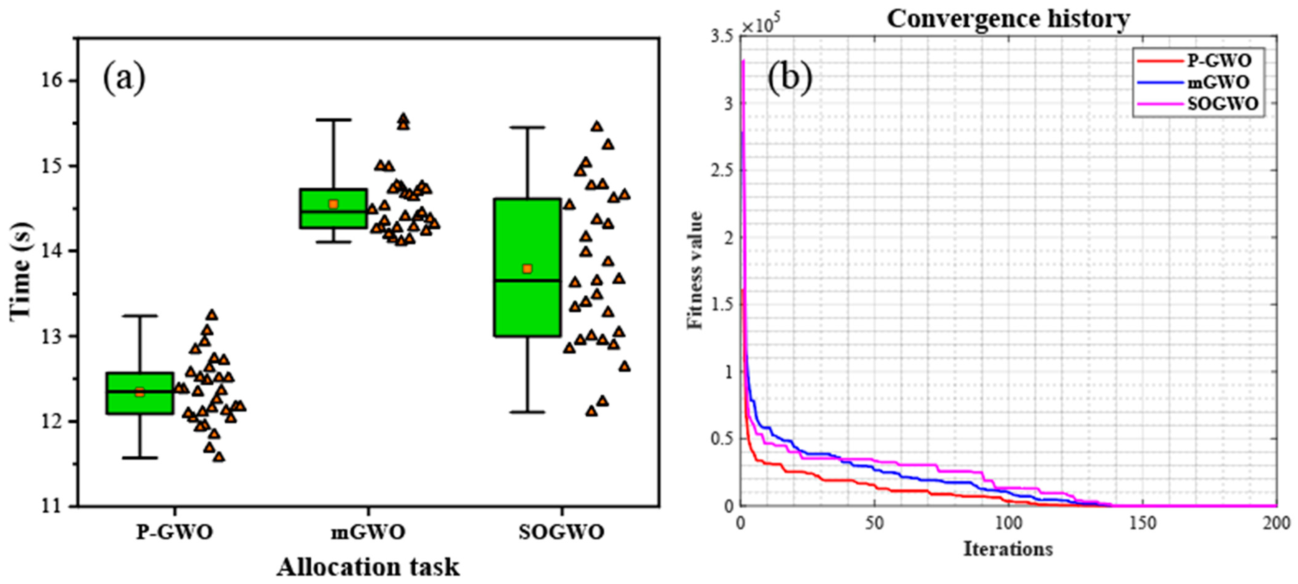
4.1. Simlation 1: Allocation Task

The entire area was defined as a 1000 m × 1000 m × −40 m space. Within this space, there were nine threat sources, each associated with a corresponding threat area. The multi-AUV scenario involved the use of four identical AUVs which began their operation from the following starting coordinates: [0, 0, −10] m, [0, 100, −10] m, [300, 0, −10] m, and [0, 300, −10] m, respectively. The coordinates of the target point were [875, 875, −10] m, [800, 875, −10] m, [875, 800, −10] m, and [800, 875, −10] m for each AUV, respectively. The velocity of the AUV ranged from 2 m/s to 3 m/s. The physical bounds of the yaw and pitch angle are $\psi \in [-\pi /3,\pi /3]$ and $\theta =[-\pi /4,\pi /4]$, respectively. $d_{safe}$ was set to be 25 m. The predefined arrival time $t_c$ was set to be 500 s.

The convergence performance of each algorithm is presented in Figure 6. As depicted in Figure 6a, the proposed P-GWO algorithm exhibits superior path planning efficiency compared to existing references, with a 10–15% lower computational time, as corroborated by the statistical results in

Table 1. Statistical results.

Methods	Average Time Cost (s)	Objective Value
P-GWO	12.321	0.292
mGWO	14.572	0.424
SOGWO	13.713	0.577

. Furthermore, the interquartile range (IQR) of P-GWO is smaller than the reference algorithms in most cases, indicating its ability to consistently produce satisfactory computational performances. The convergence data presented in Figure 6b and Table 1 demonstrate the optimality of P-GWO in solving the simulation problems, converging more rapidly to superior solutions than the other reference algorithms. The use of an adaptive decay factor and clustering strategy significantly contributes to the superior performance of the proposed P-GWO algorithm.

The experimental outcomes are visually represented in Figure 7, showing both the 2D and 3D path planning results. The presented results demonstrate the efficiency of the proposed algorithm in generating a feasible path for multi-AUVs adhering to the imposed spatial constraints. Notably, the comparative analysis of the P-GWO approach against the mGWO and SOGWO algorithms reveals its superiority in generating safer trajectories with fewer segments intersecting the designated danger zone.

Table 2. Statistical measurements for each AUV.

	Travel Distance (m)	Speed (m/s)	Arrival Time (s)	Time Windows (s)
AUV 1	1382.9	2.64	523.8	[460.9, 691.4]
AUV 2	1187.4	2.34	507.4	[395.8, 593.7]
AUV 3	1057.8	2.01	526.3	[352.6, 528.9]
AUV 4	1076.4	2.05	525.1	[358.8, 538.2]

presents the statistical measurements of the individual Autonomous Underwater Vehicles (AUVs) employed in the investigation, including their travel distance, velocities, arrival time, and time windows. The data in Table 2 reveal that the velocities of the AUVs conform strictly to the range of 2–3 m/s. Notably, the optimization algorithm utilized in the study guarantees that each AUV will arrive at its designated target within the specified time window. Furthermore, the observed arrival times of the AUVs are closely aligned, indicating effective coordination and successful execution of a joint operation. These findings demonstrate the efficacy of the employed optimization algorithm in achieving coordinated AUV missions.

4.2. Simulation 2: Rendezcous Task

In this section, the configuration space was set to 1000 m × 1000 m × −40 m. In this space, there were 13 threat areas. The starting coordinates of these four AUVs were [0, 0, −10] m, [0, 100, −10] m, [300, 0, −10] m and [0, 300, −10] m, respectively. The coordinates of the target point were [800, 800, −10] m for all AUVs. The velocity of the AUV ranges from 2 m/s to 3 m/s. The physical bound of the yaw and pitch angle are $\psi \in [-\pi /3,\pi /3]$ and $\theta =[-\pi /4,\pi /4]$, respectively. $d_{safe}$ was set to be 25 m. The predefined arrival time $t_c$ was set to be 550 s.

The convergence characteristics of the proposed P-GWO algorithm were evaluated and compared with the mGWO and SOGWO algorithms in the rendezvous tasks. The results, as presented in Figure 8 and

Table 3. Statistical results.

Methods	Average Time Cost (s)	Objective Value
P-GWO	13.406	0.374
mGWO	16.872	0.589
SOGWO	14.439	0.569

, demonstrate that P-GWO exhibits a superior computational efficiency and global searching ability compared to the reference algorithms. Specifically, P-GWO achieved a final fitness value of 0.374 while mGWO and SOGWO obtained values of 0.589 and 0.569, respectively, thus supporting the conclusions reached in Section 4.1. The visualized results presented in Figure 9 indicate that P-GWO is capable of generating safe routes for each AUV in the rendezvous tasks, with reduced potential risks posed by obstacles and enemies. Additionally,

Table 4. Statistical measurements for each AUV.

	Travel Distance (m)	Speed (m/s)	Arrival Time (s)	Time Windows (s)
AUV 1	1292.5	2.29	564.4	[430.82, 646.24]
AUV 2	1122.6	2.09	537.1	[374.20, 561.31]
AUV 3	1103.4	2.01	548.9	[367.79, 551.68]
AUV 4	1165.4	2.11	552.3	[388.45, 582.68]

provides the statistical measurements of the AUVs, indicating that all vehicles can arrive at the same target with similar arrival times of 564.4 s, 537.1 s, 548.9 s, and 552.3 s. It is important to note that the variation in arrival times of 20–30 s is deemed acceptable in a coordinated mission as the enemy typically requires more time to respond. Based on the simulation results, we can conclude that P-GWO is capable of addressing the coordinated path planning problem for AUVs in underwater coordinated missions.

5. Conclusions

The research presented in this paper offers a comprehensive exploration of coordinated path planning for multi-AUV-assisted underwater missions. It establishes a systematic model and an efficient solver capable of addressing challenges related to global optimality and quick convergence speed. Based on the obtained results, several key observations can be drawn:

• The obtained results demonstrate that the problem method proposed in combination with P-GWO is able to consistently address the coordinated path planning problem, thereby contributing to the underwater coordinated missions with specific needs;
• The present study proposes a novel coordinated path planning model for underwater coordinated missions by encapsulating various factors, including potential threats, arrival time windows, space constraints, and physical bounds for each AUV;
• Incorporating the restricted initialization and multi-objective clustering strategy, the Parallel Grey Wolf Optimizer is able to consistently address the coordinated path planning problem. The results demonstrate a 10–15% improvement in the convergence rate and a reduction of over 60% in the average cost value compared to reliable references.

References

1. Patil, P.V.; Khan, M.K.; Korulla, M.; Nagarajan, V.; Sha, O.P. Design Optimization of an AUV for Performing Depth Control Maneuver. Ocean Eng. 2022, 266, 112929. [Google Scholar] [CrossRef]
2. Topini, E.; Fanelli, F.; Topini, A.; Pebody, M.; Ridolfi, A.; Phillips, A.B.; Allotta, B. An Experimental Comparison of Deep Learning Strategies for AUV Navigation in DVL-Denied Environments. Ocean Eng. 2023, 274, 114034. [Google Scholar] [CrossRef]
3. Remmas, W.; Chemori, A.; Kruusmaa, M. Fault-Tolerant Control Allocation for a Bio-Inspired Underactuated AUV in the Presence of Actuator Failures: Design and Experiments. Ocean Eng. 2023, 285, 115327. [Google Scholar] [CrossRef]
4. Szczotka, M. AUV Launch & Recovery Handling Simulation on a Rough Sea. Ocean Eng. 2022, 246, 110509. [Google Scholar]
5. Ebrahimi, M.; Salehi, S.M. Enhancing the Dynamics of an Oceanic AUV by a Coupled-Fins-Propulsors Roll Control System. Ocean Eng. 2021, 234, 109182. [Google Scholar] [CrossRef]
6. Zhao, L.; Bai, Y.; Wang, F.; Bai, J. Path Planning for Autonomous Surface Vessels Based on Improved Artificial Fish Swarm Algorithm: A Further Study. Ships Offshore Struct. 2022, 18, 1325–1337. [Google Scholar] [CrossRef]
7. Wu, L.; Li, Y.; Liu, K.; Sun, X.; Wang, S.; Ai, X.; Yan, S.; Li, S.; Feng, X. Hydrodynamic Performance of AUV Free Running Pushed by a Rotating Propeller with Physics-Based Simulations. Ships Offshore Struct. 2021, 16, 852–864. [Google Scholar] [CrossRef]
8. Ebrahimi, M.; Kamali, A.; Abbaspour, M. Enhancing the Roll Dynamics of an AUV by Contra-Rotating-Propellers. Ships Offshore Struct. 2021, 16, 787–796. [Google Scholar] [CrossRef]
9. Ma, Y.; Hu, M.; Yan, X. Multi-Objective Path Planning for Unmanned Surface Vehicle with Currents Effects. ISA Trans. 2018, 75, 137–156. [Google Scholar] [CrossRef]
10. Zhao, L.; Bai, Y.; Paik, J.K. Global-Local Hierarchical Path Planning Scheme for Unmanned Surface Vehicles under Dynamically Unforeseen Environments. Ocean Eng. 2023, 280, 114750. [Google Scholar] [CrossRef]
11. MahmoudZadeh, S.; Yazdani, A.M.; Sammut, K.; Powers, D.M. Online Path Planning for AUV Rendezvous in Dynamic Cluttered Undersea Environment Using Evolutionary Algorithms. Appl. Soft Comput. 2018, 70, 929–945. [Google Scholar] [CrossRef]
12. Filaretov, V.; Yukhimets, D. The Method of Path Planning for AUV-Group Moving in Desired Formation in Unknown Environment with Obstacles. IFAC-PapersOnLine 2020, 53, 14650–14655. [Google Scholar] [CrossRef]
13. Khan, M.T.R.; Ahmed, S.H.; Jembre, Y.Z.; Kim, D. An Energy-Efficient Data Collection Protocol with AUV Path Planning in the Internet of Underwater Things. J. Netw. Comput. Appl. 2019, 135, 20–31. [Google Scholar] [CrossRef]
14. Li, X.; Yu, S. Three-Dimensional Path Planning for AUVs in Ocean Currents Environment Based on an Improved Compression Factor Particle Swarm Optimization Algorithm. Ocean Eng. 2023, 280, 114610. [Google Scholar] [CrossRef]
15. Tanha, S.D.N.; Dehkordi, S.F.; Korayem, A.H. Control a Mobile Robot in Social Environments by Considering Human as a Moving Obstacle. In Proceedings of the 2018 6th RSI International Conference on Robotics and Mechatronics (IcRoM), Tehran, Iran, 23–25 October 2018; pp. 256–260. [Google Scholar]
16. Hao, K.; Zhao, J.; Li, Z.; Liu, Y.; Zhao, L. Dynamic Path Planning of a Three-Dimensional Underwater AUV Based on an Adaptive Genetic Algorithm. Ocean Eng. 2022, 263, 112421. [Google Scholar] [CrossRef]
17. Sun, Y.; Gu, R.; Chen, X.; Sun, R.; Xin, L.; Bai, L. Efficient Time-Optimal Path Planning of AUV under the Ocean Currents Based on Graph and Clustering Strategy. Ocean Eng. 2022, 259, 111907. [Google Scholar] [CrossRef]
18. Vinoth Kumar, S.; Jayaparvathy, R.; Priyanka, B.N. Efficient Path Planning of AUVs for Container Ship Oil Spill Detection in Coastal Areas. Ocean Eng. 2020, 217, 107932. [Google Scholar] [CrossRef]
19. Chen, G.; Shen, Y.; Qu, N.; He, B. Path Planning of AUV during Diving Process Based on Behavioral Decision-Making. Ocean Eng. 2021, 234, 109073. [Google Scholar] [CrossRef]
20. Zhao, L.; Bai, Y.; Paik, J.K. Global Path Planning and Waypoint Following for Heterogeneous Unmanned Surface Vehicles Assisting Inland Water Monitoring. J. Ocean Eng. Sci. 2023, in press. [Google Scholar] [CrossRef]
21. Bai, G.; Chen, Y.; Hu, X.; Shi, Y.; Jiang, W.; Zhang, X. Multi-AUV Dynamic Trajectory Optimization and Collaborative Search Combined with Task Urgency and Energy Consumption Scheduling in 3-D Underwater Environment with Random Ocean Currents and Uncertain Obstacles. Ocean Eng. 2023, 275, 113841. [Google Scholar] [CrossRef]
22. Cui, R.; Li, Y.; Yan, W. Mutual Information-Based Multi-AUV Path Planning for Scalar Field Sampling Using Multidimensional RRT. IEEE Trans. Syst. Man Cybern. Syst. 2016, 46, 993–1004. [Google Scholar] [CrossRef]
23. Yu, X.; Chen, W.-N.; Hu, X.-M.; Gu, T.; Yuan, H.; Zhou, Y.; Zhang, J. Path Planning in Multiple-AUV Systems for Difficult Target Traveling Missions: A Hybrid Metaheuristic Approach. IEEE Trans. Cogn. Dev. Syst. 2020, 12, 561–574. [Google Scholar] [CrossRef]
24. Zhang, J.; Liu, M.; Zhang, S.; Zheng, R.; Dong, S. Multi-AUV Adaptive Path Planning and Cooperative Sampling for Ocean Scalar Field Estimation. IEEE Trans. Instrum. Meas. 2022, 71, 1–14. [Google Scholar] [CrossRef]
25. Chen, M.; Zhu, D. A Workload Balanced Algorithm for Task Assignment and Path Planning of Inhomogeneous Autonomous Underwater Vehicle System. IEEE Trans. Cogn. Dev. Syst. 2019, 11, 483–493. [Google Scholar] [CrossRef]
26. Mirjalili, S.; Mirjalili, S.M.; Lewis, A. Grey Wolf Optimizer. Adv. Eng. Softw. 2014, 69, 46–61. [Google Scholar] [CrossRef]
27. Emary, E.; Zawbaa, H.M.; Hassanien, A.E. Binary Grey Wolf Optimization Approaches for Feature Selection. Neurocomputing 2016, 172, 371–381. [Google Scholar] [CrossRef]
28. Radmanesh, M.; Kumar, M.; Sarim, M. Grey Wolf Optimization Based Sense and Avoid Algorithm in a Bayesian Framework for Multiple UAV Path Planning in an Uncertain Environment. Aerosp. Sci. Technol. 2018, 77, 168–179. [Google Scholar] [CrossRef]
29. Guha, D.; Roy, P.K.; Banerjee, S. Load Frequency Control of Interconnected Power System Using Grey Wolf Optimization. Swarm Evol. Comput. 2016, 27, 97–115. [Google Scholar] [CrossRef]
30. Jiaqi, S.; Li, T.; Hongtao, Z.; Xiaofeng, L.; Tianying, X. Adaptive Multi-UAV Path Planning Method Based on Improved Gray Wolf Algorithm. Comput. Electr. Eng. 2022, 104, 108377. [Google Scholar] [CrossRef]
31. Yu, X.; Jiang, N.; Wang, X.; Li, M. A Hybrid Algorithm Based on Grey Wolf Optimizer and Differential Evolution for UAV Path Planning. Expert Syst. Appl. 2023, 215, 119327. [Google Scholar] [CrossRef]
32. Jiang, W.; Lyu, Y.; Li, Y.; Guo, Y.; Zhang, W. UAV Path Planning and Collision Avoidance in 3D Environments Based on POMPD and Improved Grey Wolf Optimizer. Aerosp. Sci. Technol. 2022, 121, 107314. [Google Scholar] [CrossRef]
33. Cai, J.; Zhang, F.; Sun, S.; Li, T. A Meta-Heuristic Assisted Underwater Glider Path Planning Method. Ocean Eng. 2021, 242, 110121. [Google Scholar] [CrossRef]
34. Qu, C.; Gai, W.; Zhong, M.; Zhang, J. A Novel Reinforcement Learning Based Grey Wolf Optimizer Algorithm for Unmanned Aerial Vehicles (UAVs) Path Planning. Appl. Soft Comput. 2020, 89, 106099. [Google Scholar] [CrossRef]
35. Dhargupta, S.; Ghosh, M.; Mirjalili, S.; Sarkar, R. Selective Opposition Based Grey Wolf Optimization. Expert Syst. Appl. 2020, 151, 113389. [Google Scholar] [CrossRef]
36. Gupta, S.; Deep, K. A Memory-Based Grey Wolf Optimizer for Global Optimization Tasks. Appl. Soft Comput. 2020, 93, 106367. [Google Scholar] [CrossRef]
Figure 1. Top view of the planning space.
Jmse 11 01720 g001
Figure 2. Illustration of the path crossing the risk area.
Jmse 11 01720 g002
Figure 3. Illustration of hierarchy.
Jmse 11 01720 g003
Figure 4. Flowchart of the algorithm.
Jmse 11 01720 g004
Figure 5. Top view of the task type.
Jmse 11 01720 g005
Figure 6. (a) Time cost for each method and (b) convergence history.
Jmse 11 01720 g006
Figure 7. (a) 3D view of P-GWO; (b) 2D view of P-GWO; (c) 3D view of mGWO; (d) 2D view of mGWO; (e) 3D view of SOGWO; (f) 2D view of SOGWO.
Jmse 11 01720 g007
Figure 8. (a) Time cost for each method. and (b) convergence history.
Jmse 11 01720 g008
Figure 9. (a) 3D view of P-GWO; (b) 2D view of P-GWO; (c) 3D view of mGWO; (d) 2D view of mGWO; (e) 3D view of SOGWO; (f) 2D view of SOGWO.
Jmse 11 01720 g009