Article

Model-Parameter-Free Prescribed Time Trajectory Tracking Control for Under-Actuated Unmanned Surface Vehicles with Saturation Constraints and External Disturbances

1
Science and Technology on Underwater Vehicle Laboratory, Harbin Engineering University, Harbin 150001, China
2
No.708 Research Institute of CSIC, Shanghai 200011, China
*
Author to whom correspondence should be addressed.
J. Mar. Sci. Eng. 2023, 11(9), 1717; https://doi.org/10.3390/jmse11091717
Submission received: 31 July 2023 / Revised: 25 August 2023 / Accepted: 29 August 2023 / Published: 31 August 2023

Abstract

:
This paper mainly addresses the model-parameter-free prescribed time trajectory tracking control issue for under-actuated unmanned surface vehicles (USVs) that are susceptible to model uncertainties, time-varying disturbances, and saturation constraints. Firstly, a state extension based on coordinate transformation was designed to address the lack of control in the sway channel. Secondly, nonlinear behavior stemming from saturation constraints is not always differentiable. Regarding this, a smooth dead-zone-based model was conducted to fit the behavior, leaving a relatively simple actuator model. Then, an improved prescribed time–prescribed performance function (PTPPF) and error transformation method were utilized to propose a model-parameter-free control algorithm that guarantees user-defined constrained boundaries while ensuring all tracking errors converge within small domains before a preassigned settling time. The theoretical analysis was conducted by the initial value theorem, Lyapunov’s second method, and proof by contradiction, followed by comparative simulation results that verified the effectiveness of the proposed control scheme.

1. Introduction

USVs, which possess autonomous decision-making and task-execution capabilities, have found significant applications in various fields. Recently, due to the USV’s autonomy and flexibility, they are used in marine scientific research, maritime surveillance, and resource exploration [1,2,3,4]. In practical marine environments, USVs encounter constantly changing weather conditions, waves, currents, and obstacles. To cope with these environmental uncertainties, the controller needs to employ robust control algorithms that can adapt to different conditions. As control technology continues to advance and innovate, several advanced control theories, such as sliding mode control (SMC) [5,6,7,8] and back-stepping control [9,10], have been applied to enhance trajectory tracking control for USVs.
Eminent characteristics of transient and steady state are significant for the whole system, such as small maximum overshoot and steady-state error. However, compared with the prescribed performance control (PPC), the aforementioned control schemes need time-consuming parameter modifications to satisfy appropriate performance. The concept of PPC was first proposed in ref. [11]. As an effective control method considering prior performance constraints, PPC adopts the output error transformation method, and the prescribed performance function (PPF) can achieve the specified satisfactory value of the control performances. By integrating other control methods, PPC is extensively implemented in many fields. For instance, an adaptive prescribed-performance controller was described, utilizing an efficient combination of multi-layer neural networks [12]. The work proposed an adaptive SMC strategy that provides asymptotic stability and tracking performance in finite time [13]. Moreover, other control methods such as back-stepping control [14,15] and SMC [16,17] also can be used in combination with PPC.
The study [18] developed a unique prescribed performance function to ensure timely convergence for systems with time-varying inner coupling. This method allows the tracking errors to remain within the specified performance bounds at the user-defined time. Similarly, in order to achieve timely convergence for systems with time-varying inner coupling, ref. [19] introduced a novel prescribed performance function that enables the controller to drive the error to converge within the user-defined time. However, it is important to note that the aforementioned methods often assume that the initial tracking error is small, which may not always be applicable in practical systems. Taking this into consideration, ref. [20] proposed a new error transformation method and a revised performance function. The key concept is to set the initial value of the performance constraint boundary to infinity, ensuring that the tracking error at the beginning falls within the permissible performance limitations. This approach relaxes the requirement of the performance function to depend on the initial error.
The majority of the prescribed performance control (PPC) methods mentioned above rely on approximation techniques such as neural networks (NN) and fuzzy methods to estimate the unknown dynamics of the model and subsequently facilitate the design of the corresponding controllers. As a consequence, the selection of adaptive laws for numerous unknown parameters poses challenges in implementing the designed control law in on-line adjustment. Although the low-complexity method of prescribed performance control has obtained many achievements [21,22], more simple and effective model-free control schemes still need to be studied.
In practical environments, controllers for unmanned surface vehicles (USVs) are constrained by physical limitations, with saturation constraints being the primary factor affecting the precision of the USV system’s control. When the control output command exceeds the actuator’s rated value, the state may be inaccurately updated, resulting in a potential degradation of the system’s performance. To address the adverse effects caused by saturation constraints, various solutions have been proposed. One approach involves the design of an additional anti-saturation auxiliary system [23], which is specifically activated when saturation occurs. Moreover, another way is to design a proper saturation model; ref. [24] directly adopted the traditional hard saturation model, which conformed to reality, but due to its non-differentiability, it cannot effectively deal with the nonlinear term caused by saturation. In light of this, a differentiable saturation function proposed in ref. [25] and a new dead-zone nonlinearities saturation model introduced in ref. [26] aimed to ensure system stability and safety. However, when combined with PPC technology, the mathematical derivation becomes intricate. There are alternative simple models available, such as the Gaussian error function [27] and the hyperbolic tangent function [28], which are easy to derive. However, they do not integrate well with the control model. To address these concerns, we introduce a dead-zone operator-based model, which offers the advantage of employing a linear approach.
In the actual ocean environment, USVs are significantly influenced by external disturbances, leading to a decrease in trajectory tracking accuracy. In this regard, it is crucial to emphasize the robustness of the USV system. The study [29] achieved fast and precise control of the system states by introducing a sliding surface and exhibits strong robustness against system parameter uncertainties and external disturbances. The study [30] introduced a novel observer to calculate disturbances, hence enhancing the tracking accuracy and robustness, in order to address unknown disturbances that impact the system stability. To simplify the complexity of parameter adjustment, ref. [31] introduced a useful adaptive controller based on the adaptive super-twisting method. This controller only requires the adjustment of a single parameter. In order to handle multiple uncertainties within a fixed time and account for unknown disturbances and uncertainties, ref. [32] proposed the use of an extended-state observer (ESO). To estimate velocities and perturbations, a nonlinear ESO was proposed, and based on this, an adaptive neural network (NN) was suggested to evaluate the unknown terms [33]. In another work [34], a reduced-order ESO was introduced to estimate external disturbances.
This work proposes a robust model-parameter-free anti-saturation control algorithm for trajectory tracking control of under-actuated USVs relying on the back-stepping control design method. Then, the contributions of this article are presented here:
(1)
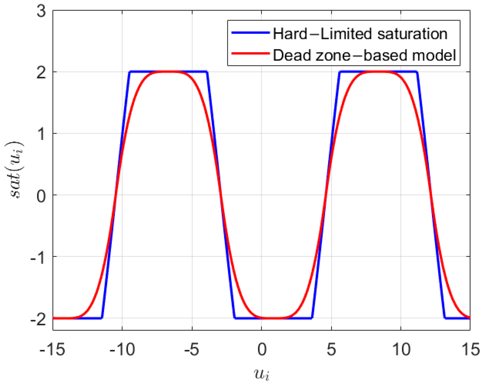
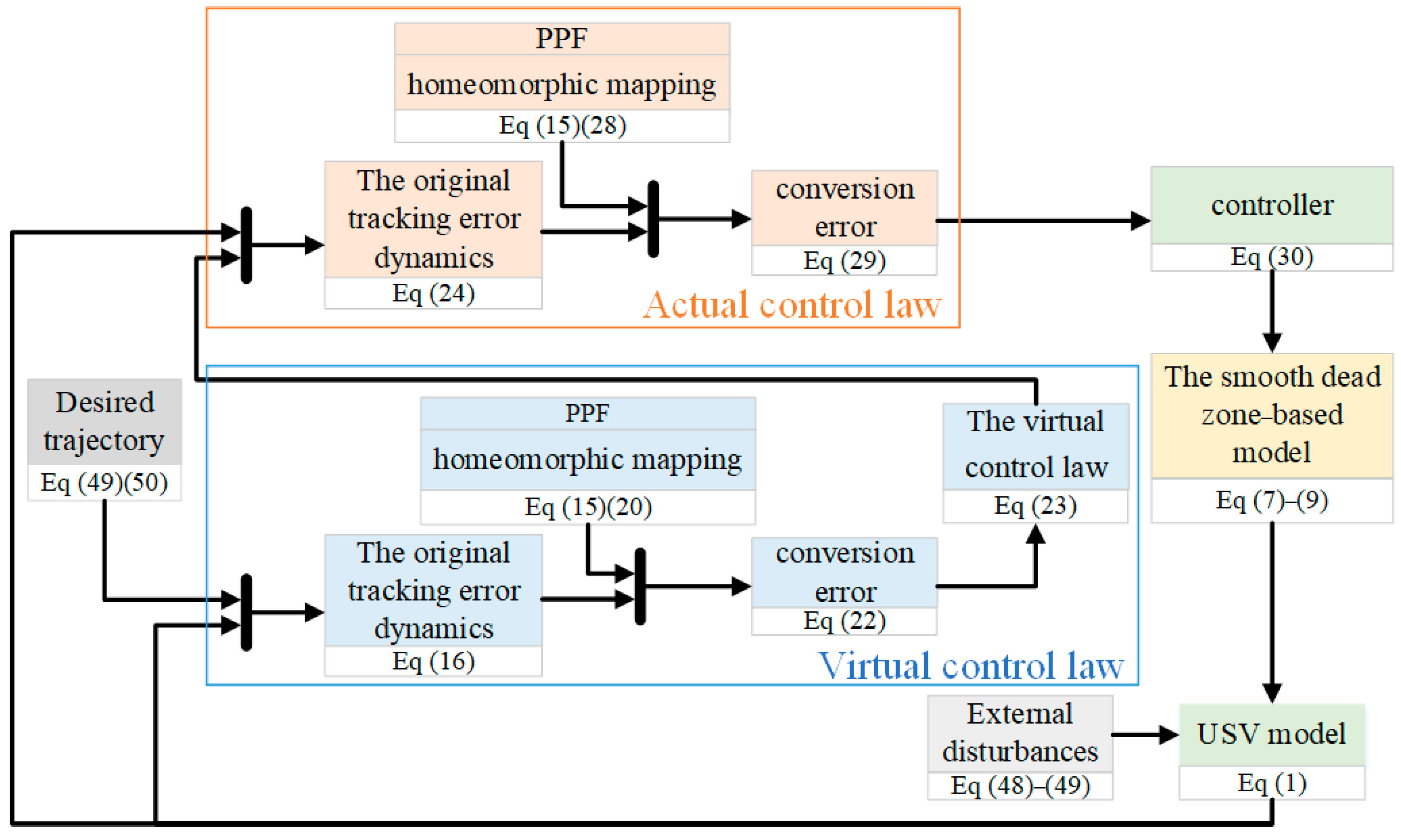
Considering the under-actuated nature of the unmanned vehicle, where there is no independent actuator in the swaying velocity direction, the direct application of feedback linearization becomes challenging. In this paper, a state-extension technique based on coordinate transformation is employed to rewrite the control model. Additionally, the potential negative impact of saturation constraints on control stability is addressed by utilizing a smooth dead-zone-based model instead of the conventional hard saturation model. This approach not only facilitates the subsequent controller design but also ensures the control stability in the presence of saturation constraints;
(2)
In the trajectory tracking control of under-actuated USVs, a model-parameter-free controller is utilized, simplifying the design process by reducing the number of adjustable parameters. By employing the back-stepping control design process, it is demonstrated that the proposed control mechanism performs effectively within the specified performance framework. Moreover, the convergence time can be specified, allowing for the desired control performance to be achieved within a predefined timeframe.
The content in this document is arranged as follows: The corresponding mathematical models for the USV and saturation constraint are presented in Section 2. The design of a model-free parameter controller is presented in Section 3, together with the accompanying stability proofs using the initial value theorem, Lyapunov’s second method, and the proof by contradiction. Comparative simulation outcomes are shown in Section 4. Section 5 provides a conclusion to the essay.

2. Problem Formulation

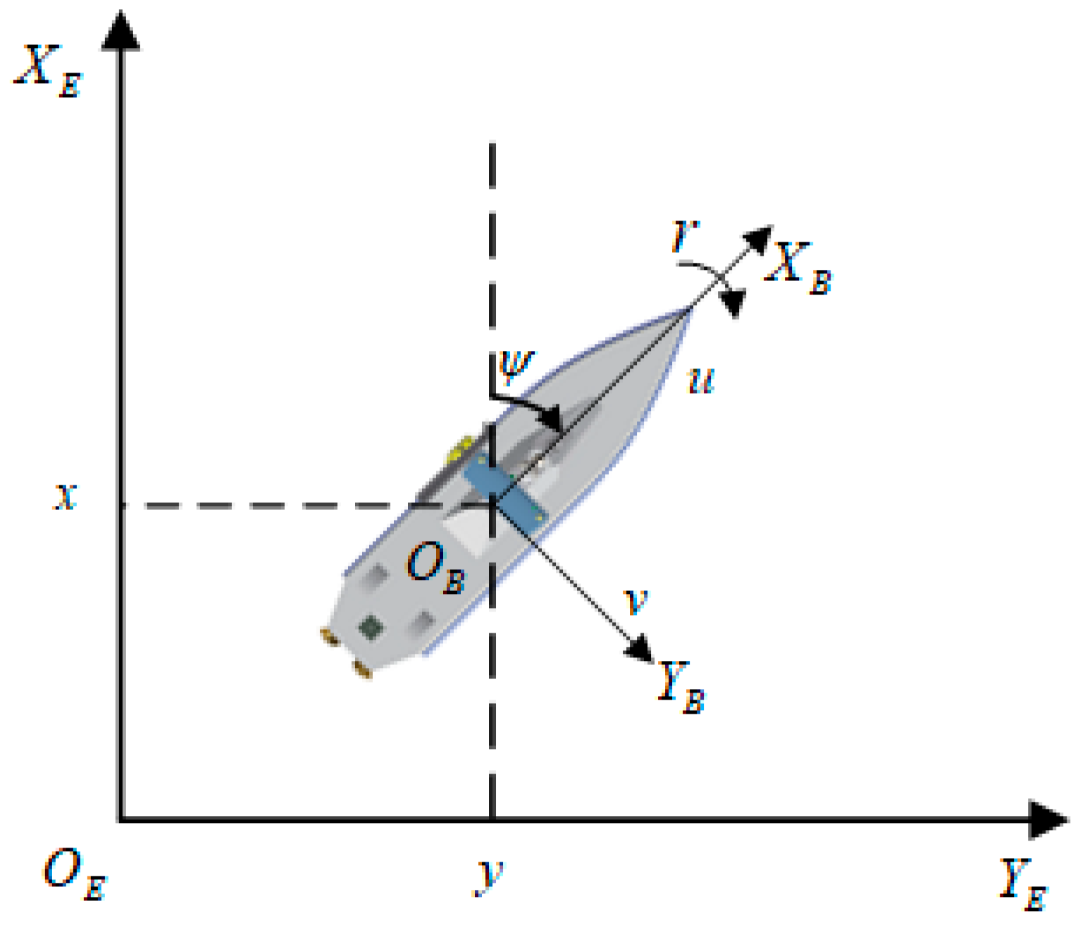
2.1. Dynamics of Under-Actuated USV

In order to express the motion of USV, two coordinates frame  X E O E Y E and  X B O B Y B are illustrated in Figure 1.
The entire system is provided for an under-actuated USV subject to saturation constraints, time-varying disturbances, and parametric uncertainties.
x ˙ y ˙ ψ ˙ = cos ψ sin ψ 0 sin ψ cos ψ 0 0 0 1 u v r
m 11 0 0 0 m 22 0 0 0 m 33 u ˙ v ˙ r ˙ + 0 0 m 22 v 0 0 m 11 u m 22 v m 11 u 0 u v r + d 1 u h 1 d 2 v h 2 d 3 sgn r r h 3 = τ u 0 τ r + τ d u τ d v τ d r
where  x , y represents the position of USV in the earth-fixed frame  X E O E Y E , and  ψ represents the yaw angle;  u stands for the surge velocity,  v stands for the sway velocity, and  r stands for the angular velocity;  d i a g m 11 , m 22 , m 33 represents the inertia mass,  d 1 u h 1 , d 2 v h 2 , d 3 sgn r r h 3 T represents the hydrodynamics damping term, and  d i , h i i = 1 , 2 , 3 are nonlinear damping parameters;  τ u and  τ r denote the control force/torque generated by the propeller, taking into account input saturation constraints;  τ d i i = u , v , r denotes the external lumped disturbances. For more information about this model, please refer to ref. [35].
The system kinematics are now rewritten by a state extension based on coordinate transformation, which is different from the commonly used origin point of the body-fixed frame. For the under-actuated USV, a new vector is defined as follows [36]:
ζ 1 = x + l cos ψ ζ 2 = y + l sin ψ
where  l is the designed parameter.
Remark 1.
In the original 3-degree-of-freedom trajectory tracking system for the under-actuated USV, two control inputs were used to control the tracking errors in the x-direction, y-direction, and heading. By introducing a state extension based on coordinate transformation, the x-direction tracking error and y-direction tracking error now incorporate the heading angle. As a result, it becomes possible to control both the x-direction tracking error and y-direction tracking error using only two control inputs while also achieving control over the heading angle. It is important to note that the method may introduce additional coupling effects due to the offset. Therefore, choosing an appropriate designed parameter  l should be considered in the controller design to ensure satisfactory control performance of the heading angle.
For convenience, we set  ζ = ζ 1 , ζ 2 T and  σ = ζ ˙ 1 , ζ ˙ 2 T . By taking the derivative of Equation (3) and combining it with Equation (1), we obtain the following result:
ζ ˙ = σ σ ˙ = Λ τ + Γ + Λ d
with  τ = τ u , τ r T d = τ d u , τ d r T ,
Λ = cos ψ m 11 l sin ψ m 33 sin ψ m 11 l cos ψ m 33 ,   f u = m 22 / m 11 v r d 1 u h 1 / m 11 f v = m 11 / m 22 u r d 2 v h 2 / m 22 f r = m 11 m 22 / m 33 u v d 3 sgn r r h 3 / m 33
Γ = f u cos ψ u r sin ψ v r cos ψ f v + τ d v / m 22 sin ψ f u sin ψ + u r cos ψ v r sin ψ + f v + τ d v / m 22 cos ψ + l f r sin ψ + l r 2 cos ψ l f r cos ψ l r 2 sin ψ
The following theorem is made to simplify the design process.
Theorem 1.
The time-varying disturbances and their first derivatives are bounded;  τ d i τ ¯ d i τ ˙ d i τ ˙ ¯ d i , and  i = u , v , r , and  τ ¯ d i  and  τ ˙ ¯ d i  are constants. This assumption is frequently used in the literature [37,38] when designing controllers.
Remark 2.
In practice, the control torque and the speed of the USV cannot be infinite, and there must be corresponding upper bounds, combined with the condition that the time-varying external disturbances are bounded in Assumption 1, so the terms  Λ and  Γ are both bounded.

2.2. Saturation Constraints

Here, we take into consideration the output limitations of the USV’s actuator, specifically the propeller. Particularly during the initial stages of tracking the desired trajectory, there may be larger control commands that the propeller cannot accommodate, resulting in the occurrence of saturation constraints.
Consider the actuator of under-actuated USV with saturation constraints; the control vector  τ i is defined as follows [39]:
τ i = sign τ i c min τ i c , τ i max
where  τ i c is the command input, and  τ i max is the maximum allowable control force and moment of the corresponding input. It is indifferentiable at  τ i = τ i max from the expression of saturation constraints (7). Thus, a smooth dead-zone-based model (8)–(10) is used as a limiting filter to guarantee the desired control accuracy while the USV model is affected by saturation constraints [40].
φ τ c i = n i τ c i g i ,   i = u , r
g i = 0 α i l i β z τ c i , β d β ,   i = u , r
z τ c i , β = max τ c i β , min 0 , τ c i + β
where  n i = 0 α i l i β d β is a positive constant with  α i > 0 is a parameter to be designed;  𝓁 l i β ,   i = u , r is a density function satisfying  l i β 0 ; note that  g i is bounded, and this property will be confirmed in the proof of Lemma 1.
Lemma 1.
There always exists a density function  l i β  such that the following equation applies for any maximum permitted control input  τ i max :
τ i max = lim τ c i φ τ c i = 0 α i β l i β d β
Proof. 
From our definition of  z τ c i , β , we can derive the following:
lim τ c i z τ c i , β = τ c i β
Further, by substituting the Formulas (9) and (11) into the Formula (7), we can obtain the following:
lim τ c i φ τ c i = n i τ c i 0 α i τ c i l i β d β + 0 α i β l i β d β
Based on the definition of  n i and Equation (8), Equation (11) can be derived. Additionally, from Formula (13), it can be inferred that  φ τ c i must be bounded because it is a continuous function, so  g i is also bounded. The curve defined by saturation constraints remains smooth in Equations (8)–(10), as depicted in Figure 2. In contrast, the traditional method (7) is deemed less optimal. □
The saturation constraint of actuator ultimately is modified as follows based on (8)–(10):
τ = n τ c g + δ
where  n = d i a g n u , n r g = [ g u , g r ] T , and  δ = [ δ u , δ r ] T are the parameters.  δ = τ i φ τ c i is the filtering error. It is evident that although this term  δ is unknown, Lemma 1 implies that it is bounded. Combining Equations (4) and (14), we obtain the following model:
ζ ˙ = σ σ ˙ = Λ n τ c + Γ + Θ
where  Θ = Λ d g + δ .
The model-parameter-free control architecture is described in Section 3; however, it should be noted that  Γ and  Θ include the USV-related parameters, which are both unavailable to the designer here.
Remark 3.
The dead-zone-based model (14), as defined in [40], effectively captures the saturation limits in various scenarios. Moreover, the linearity of the system enables the application of robust and adaptive control techniques.

2.3. Prescribed Time–Prescribed Performance Function

The following definition is given to show the criterion of PPF:
Definition 1
([41]). A continuous function  ρ t : 0 , + +  will be called as the PPF if it satisfies the following:
(1) 
For any  t > 0 ,  ρ t  is a positive function;.
(2) 
The function  ρ t  is monotonic decreasing on the interval  0 , T p ;
(3) 
The equation  ρ t ρ > 0  holds  t > T p .
By referring to [20], a piecewise function is given:
ρ t = csc π ( t + c ) 2 t t ρ _ ρ ¯ t + t p t p 1 1 γ + ρ ¯ ,   0 t < t t c t + t p t p 1 1 γ ρ _ ρ ¯ + ρ ¯ ,   t t c t < t p ρ ¯ ,   t t p
where  c is a positive constant;  γ is between zero and one, which influences the PPF’s rate of decline;  t t ( c , t p ) represents the transition time; and  t p stands for the settling time. The PTPPF ensures that the tracking error converges to the stable domains within the stable time  t p while also maintaining it within the defined performance limitations. It is evident that Equation (16) satisfies Definition 1.
Remark 4.
The detailed proof of the reasonableness of the PTPPF can refer to the work [20]. Two parameters related to time constraints are introduced in (16), the user-defined settling time  t t  and the transition time  t p . According to the different requirements,  t p  is selected as the allowable error convergence time, and  t s  should be less than the time when the error enters the range contained in the prescribed performance function. Making a decision about the balance between the two parameters is important since lower  t t  and  t p  result in a shorter stable time and a stronger control signal.

2.4. Control Objective

To proceed, we define  ζ d = x d , y d T as the desired trajectory in the frame  X E O E Y E , so the error variable  ζ e can be defined as follows:
ζ e = ζ ζ d
Therefore, the goal of control is to design the controller  τ such that the closed-loop error system satisfies the prescribed performance.
Assumption 1.
The trajectory  ζ d  is a user-designed function, so  ζ d  and  ζ ˙ d  are bounded, and  ζ ¯ d  and  ζ ˙ ¯ d  are constants.

3. Model-Parameter-Free Controller Design

Firstly, similar to the design steps in the literature [42], the normalized tracking error is defined as given:
e 1 = ζ e / ρ 1
where  e 1 = e 1 u , e 1 r T , and  e 1 i 0 < 1 . As a result, it is implied that the tracking error  e 1 always remains exactly inside the acceptable performance limit and at the prescribed time.
The derivative of (18) yields the following:
e ˙ 1 = ρ 1 2 ζ ˙ e ρ 1 ζ e ρ ˙ 1
By employing (17) and (18), Equation (18) can be obtained:
e ˙ 1 = ρ 1 1 σ ρ 1 1 ζ ˙ d ρ 1 2 ζ e ρ ˙ 1
The constraint-free tracking error is derived by applying homeomorphic mapping:
w 1 = 1 2 ln 1 + e 1 1 e 1
Based on (19) and (20), the derivative of (21) yields the following:
w ˙ 1 = e ˙ 1 1 e 1 2 = ζ ˙ e ρ 1 ρ ˙ 1 ζ e ρ 1 2 ζ e 2 = ρ 1 2 e ˙ 1 ρ 1 2 ζ e 2
Then, we have the following:
ζ e = ρ 1 t tanh w 1
If  w 1 is bounded, we have  ζ e < ρ 1 t t > 0 with the application of the  tanh · function. Then the first virtual control law is designed:
σ d = k 1 w 1
where  σ d = σ d u , σ d r T k 1 = d i a g k 1 u , k 1 r ,   k 1 i > 0 , and  w 1 = w 1 u , w 1 r T .
Then we define another tracking error as given:
σ e = σ σ d
where  σ e = σ e u , σ e r T . Then, an auxiliary variable is defined as follows:
e 2 = σ e / ρ 2
where  e 2 = e 2 u , e 2 r T , and the derivative of (26) according to time yields the following:
e ˙ 2 = ρ 2 2 σ ˙ σ ˙ d ρ 2 σ σ d ρ ˙ 2
By employing (15), (25), and (26), Equation (27) can be obtained:
e ˙ 2 = ρ 2 1 Λ n τ c + Γ + Θ ρ 2 1 σ ˙ d ρ 2 1 e 2 ρ ˙ 2
The error transformation mapping is obtained as given:
w 2 = tan π 2 e 2
where  w 2 = w 2 u , w 2 r T , which is a smooth and invertible function. From the inverse transformations of  w 2 , one can derive the following:
σ e = 2 π ρ 2 arctan w 2
If  w 2 is bounded, then applying the  arc tan · function results in  σ e < ρ 2 t t > 0 , which indicates that the error  σ e strictly grows inside the specified performance threshold.
The model-parameter-free control law based on the modified back-stepping control design process is designed:
τ c = k 2 n 1 Λ 1 W T w 2
W = 2 π diag w 2 u σ e u , w 2 r σ e r ,   w 2 i σ e i = π 2 ρ 2 i cos 2 π 2 e 2 i 1 , i = u , r w 2 T W = tan π 2 e 2 / ρ 2 cos 2 π 2 e 2
Remark 5.
The term  k 2 W T w 2  in model-parameter-free control law (31) is introduced to enforce the stability of the error transformation Equation (29) and make sure that the variable  w 2  in Equation (28) remains within the desired performance boundaries. It is important to note that our controller is model- parameter-free and does not require complex computations. The absence of system parameters in the controller’s expression enhances its simplicity and flexibility in practical applications.
To continue, a vital definition and lemmas are given:
Definition 2.
Consider the initial value problem:
μ ˙ t = y t , μ t , μ 0 Ω μ
where  Ω μ R n  is a non-empty open set, and  y : Ω μ × R + , 0 R n  is a locally integrable function. If a solution to the initial value issue (33) is also a solution to (33) and has no correct extension, then it is maximum.
Lemma 2.
Based on Definition 2, assume that  y  is continuous and locally integrable on  t  for each fixed  μ Ω μ , and  h  is locally Lipschitz on  μ . Then, there exists a unique maximal solution  μ t Ω μ  in the domain  0 , T  of the system with  T > 0  such that all solutions for any  t  belongs to  0 , T  are on the set  Ω μ .
Lemma 3.
Assume that the hypotheses of Theorem 2 hold. For a unique maximal solution,  μ Ω μ  is defined in the domain  0 , T . If  T < + , then for any compact set  Ω μ Ω μ , there exists a time instant  t * 0 , T  such that  μ t * Ω μ .
For the sake of conciseness, the extensive proofs that are provided in [43] are omitted in this study.
Following the virtual control laws (24), the derivative of  e 1 finally yields the following:
e ˙ 1 = ρ 1 1 σ e k 1 w 1 ρ 1 1 ζ ˙ d ρ 1 1 e 1 ρ ˙ 1
According to the above analysis and design, we know that  ρ 1 ρ ˙ 1 , and  e 1 are continuous and locally integrable on  t . Furthermore,  e 1 < 1 is locally Lipschitz over  Ω e 1 = 1 , 1 if we choose a small  l . As a result, we can assert there exists  e 1 Ω e 1 for any  t that belongs to  0 , T of system (34). We know that the terms  ζ e and  ζ ˙ e are bounded for  t 0 , T , and we have the following:
ρ 1 , t ρ 1 t csc π l 1 2 t t 1 ρ 1 , 0 csc π l 1 2 t t 1 π cot π l 1 / 2 t t 1 2 t t 1 1 t p 1 1 γ 1 ρ 1 , 0 ρ 1 , ρ ˙ 1 t 0
Differentiating  σ d and substituting (22), we have the following:
σ ˙ d = k 1 ρ 1 ρ 1 2 ζ e 2 ζ ˙ e e 1 ρ ˙ 1
One can easily argue that  σ ˙ d is bounded for  t 0 , t max . As a result, we can claim that there exists  e 2 Ω e 2 for any  t 0 , T of the system (28),  Ω e 2 = 1 , 1 .
Then, we have the following:
V 1 = w 1 w 1 T / 2
Substituting (22) and (34) into (37), one can derive the following:
V ˙ 1 = w 1 1 ρ 1 1 e 1 2 σ e + σ d ζ ˙ d e 1 ρ ˙ 1
Utilizing the definition of  σ e in Equation (25) and the fact that  1 / 1 e 1 2 1 , we have  max σ e ζ ˙ d e 1 ρ ˙ < Δ 1 , t 0 , t max . For any  t , we can obtain the following:
V ˙ 1 w 1 1 ρ 1 1 e 1 2 Δ 1 k 1 w 1
Therefore, we know that  V ˙ 1 0 when  Δ 1 k 1 w 1 < 0 and can subsequently infer the following:
V 1 max V 1 0 , Δ 1 2 2 i = 1 2 k 1 2 ,   t [ 0 , T ) max w 1 i i = 1 2 max w 1 i 0 , 2 Δ 1 λ min K 1
Then, we choose the following:
V 2 = 1 π w 2 T w 2
Substituting (26) and (31) into (41), one can derive the following:
V ˙ 2 = 2 π w 2 T π 2 ρ 2 cos 2 π 2 e 2 1 Λ n τ c + Γ + Θ σ ˙ d e 2 ρ ˙ 2 ρ 2 1 = w 2 T W Λ n τ c + Γ + Θ σ ˙ d e 2 ρ ˙ 2 ρ 2 1 w 2 T W Γ + Θ e 2 ρ ˙ 2 ρ 2 1 + σ ˙ d k 2 w 2 T W W T w 2
With (31), we can obtain the following:
w 2 T W 2 max ρ 2 i 2 0 i = 1 2 tan 2 π 2 e 2 i
According to Remark 1 and the above analysis, we can conclude the term in Formula (41)  Λ g + Γ + Θ σ ˙ d e 2 ρ ˙ 2 is bounded:
Γ + Θ e 2 ρ ˙ 2 + σ ˙ d < Δ 2 , t 0 , T
And (42) can be further rewritten as given:
V ˙ 2 w 2 T W k 2 w 2 T W + Δ 2 , t 0 , T
From (45), we can conclude that  V ˙ 2 is negative for any  w 2 T W 2 > Δ 2 / k 2 . Then, we can obtain the following:
V 2 t max V 2 0 , Δ 2 2 π i = 1 2 k 2 2 , t [ 0 , T ) w 2 max π V 2 0 , 2 Δ 2 λ min K 2 ,   t [ 0 , T )
On the basis of the stability analysis, it is obvious that  Ω e 1 × Ω e 2 1 , 1 ; if we assume that  T is less than positive infinity, a time instant  t ¯ belongs to  0 , T exists such that  e i t ¯ Ω e 1 × Ω e 2 , which is contradictory to what is expressed in Definition 2, and then, we can conclude that  T = + . As a consequence, in the presence of saturation constraints, the system’s tracking errors converge within the given time to satisfy the performance requirements. Additionally, Figure 3 shows a schematic of the model-parameter-free controller.

4. Simulations

We utilized MATLAB 2022a and Simulink for numerical simulations, which were conducted to testify the correctness of the proposed control scheme.
To proceed, an under-actuated unmanned surface vessel was chosen as the simulation model, whose length is 0.45 m and weight is 1.614 kg. The model parameters are given as follows [35]:  m 11 = 1.956 m 22 = 2.405 m 33 = 0.043 d 1 = 2.436 d 2 = 12.992 d 3 = 0.0564 h 1 = 2.51 h 2 = 2.747 , and  h 3 = 2.592 . Furthermore, the parameter of Formula (3) was chosen as  l = 0.01 . Three different disturbances of the time-varying ocean are shown:
Case 1:
τ d = 3 100 sin ( 1 2 t ) cos ( 1 2 t ) 1 5 cos ( t ) cos 1 2 t 3 10 1 100 sin 1 10 t 6 100 sin 11 10 t cos ( 3 10 t )
Case 2:
τ d = 0.2 sin π / 3 + 0.2 π t cos ( 0.1 t ) 0.05 sin 0.5 π t 0.3 0.12 sin 1.1 π t + π / 5   i f   t 20 s sin 0.2 π t cos 0.5 t 1.9 + 0.1 cos 0.5 t 0.6 sin 0.9 π t π / 6   i f   20 s < t 40 s 1.5 cos 0.2 π t + 0.4 0.2 cos 0.5 t 0.6 sin 0.9 t cos π t   i f   t > 40 s
Case 3:
ζ ˙ 1 i = ζ 2 i ζ ˙ 2 i = μ i 2 ζ 1 i 2 ƛ i κ i ζ 2 i + σ i α i d i = ζ 2 i
where  κ i = 0.8976 ƛ = 0.1 ,and  σ i = 1.0 .
The actuators’ maximum allowable force and torque were chosen as  τ i max = 4 N and  i = u , r . The density function was chosen as  l β = max χ i sign α i β , 0 with  α i = 8 and  χ i = 0.125 .
To ensure that the system performance converged within a specified time, the parameters of the prescribed performance function were selected as  ρ _ = 4 ρ ¯ = 0.08 γ = 0.5 c = 0.01 , and  t t = 8 t p = 10 , and the control gains are  k 1 = d i a g 3.5 , 3.5 and  k 2 = 0.5 .

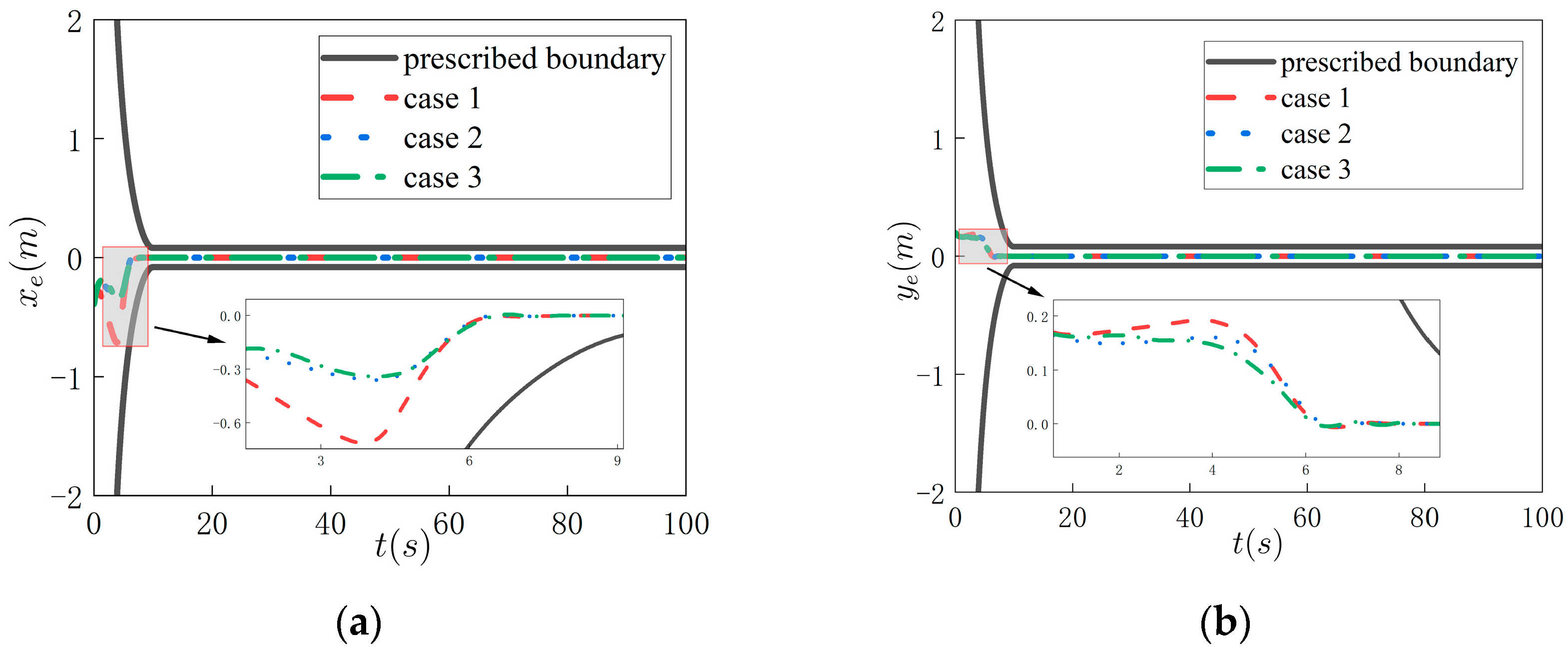
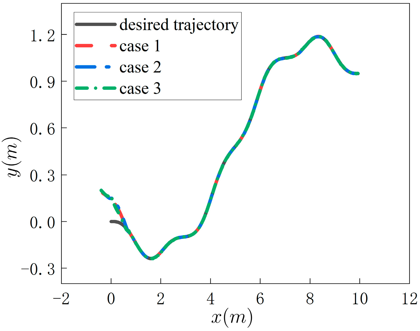
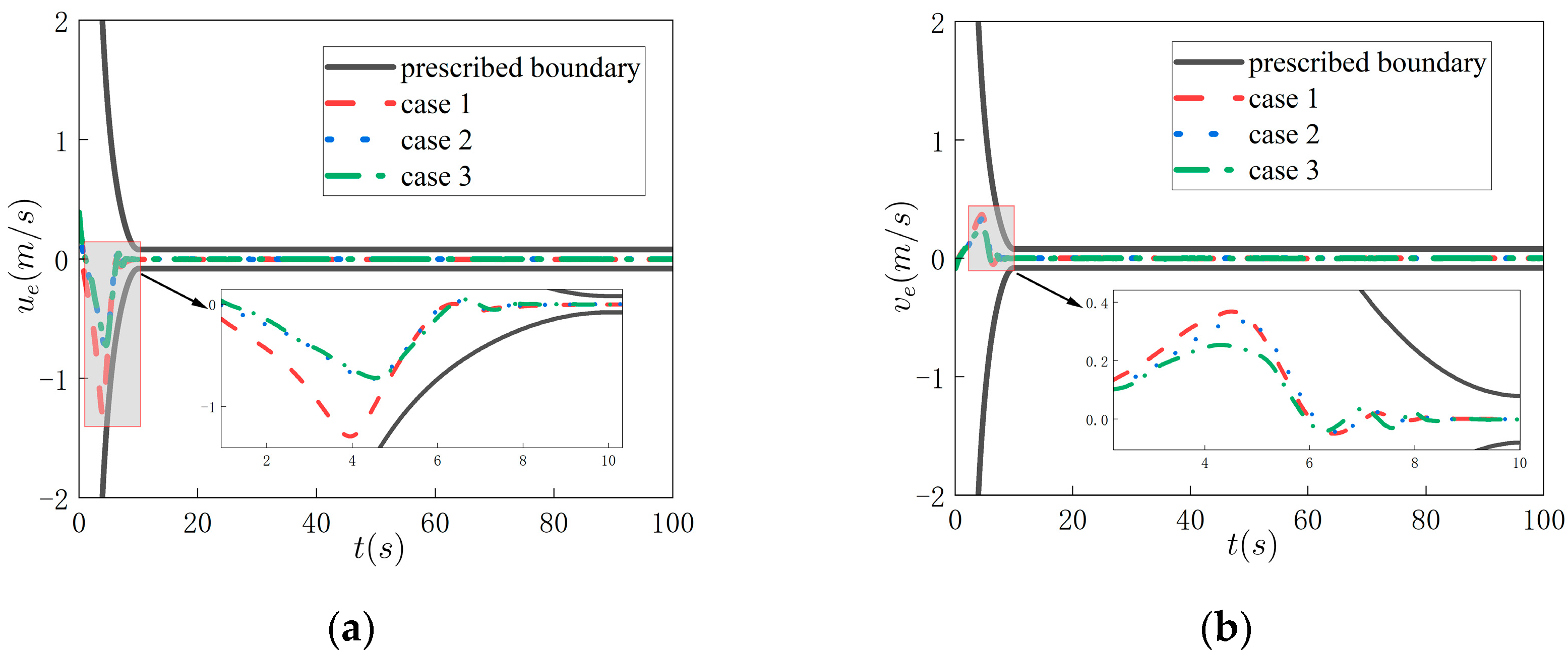
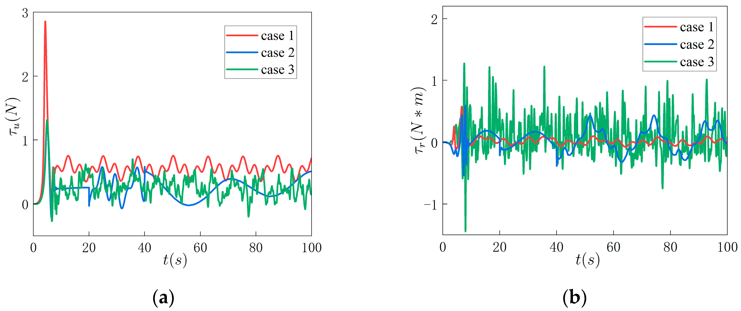
4.1. Robustness Verification

The first numerical simulation aimed to validate the robustness of the presented control approach in the presence of diverse current and wave scenarios. The desired trajectory is defined:
η ˙ d = cos ψ d sin ψ d 0 sin ψ d cos ψ d 0 0 0 1 u d v d r d
where  u d = 0 t 0.001 cos 0.15 π t d t v d = 0 t 0.005 sin 0.1 π t d t , and  r d = 0 t 0.001 cos 0.02 π t d t are user-defined velocities, and the initial states are set as  η 0 = 0.4 , 0.2 , π / 18 T u 0 = 0.8 v 0 = 0.1 , and  r 0 = 0.05 .
Remark 6.
The selection of a curved trajectory (49) aligns with the practical requirements of unmanned boat operations and provides a realistic representation of the challenges faced in ocean scenarios. Furthermore, it allows for a comprehensive assessment of the controller’s performance in a dynamic environment. The chosen trajectory serves as an appropriate benchmark to assess the effectiveness and robustness of the proposed controller in tracking complex.
The simulation results under three cases are shown in Figure 4, Figure 5, Figure 6 and Figure 7. Figure 4 illustrates the trajectory of the USV under these three cases. The tracking errors  x e , y e , u e , v e are shown in Figure 5 and Figure 6, respectively. It can be observed from the partially enlarged detail in the figures that the tracking errors converged within the prescribed boundaries with satisfactory convergence speed. The evolution of control inputs is displayed in Figure 7. Under the same control settings, it is evident that the magnitude of the input was influenced by high-frequency and greater external disturbances. In these figures, the high-precision performance of the controller is guaranteed.

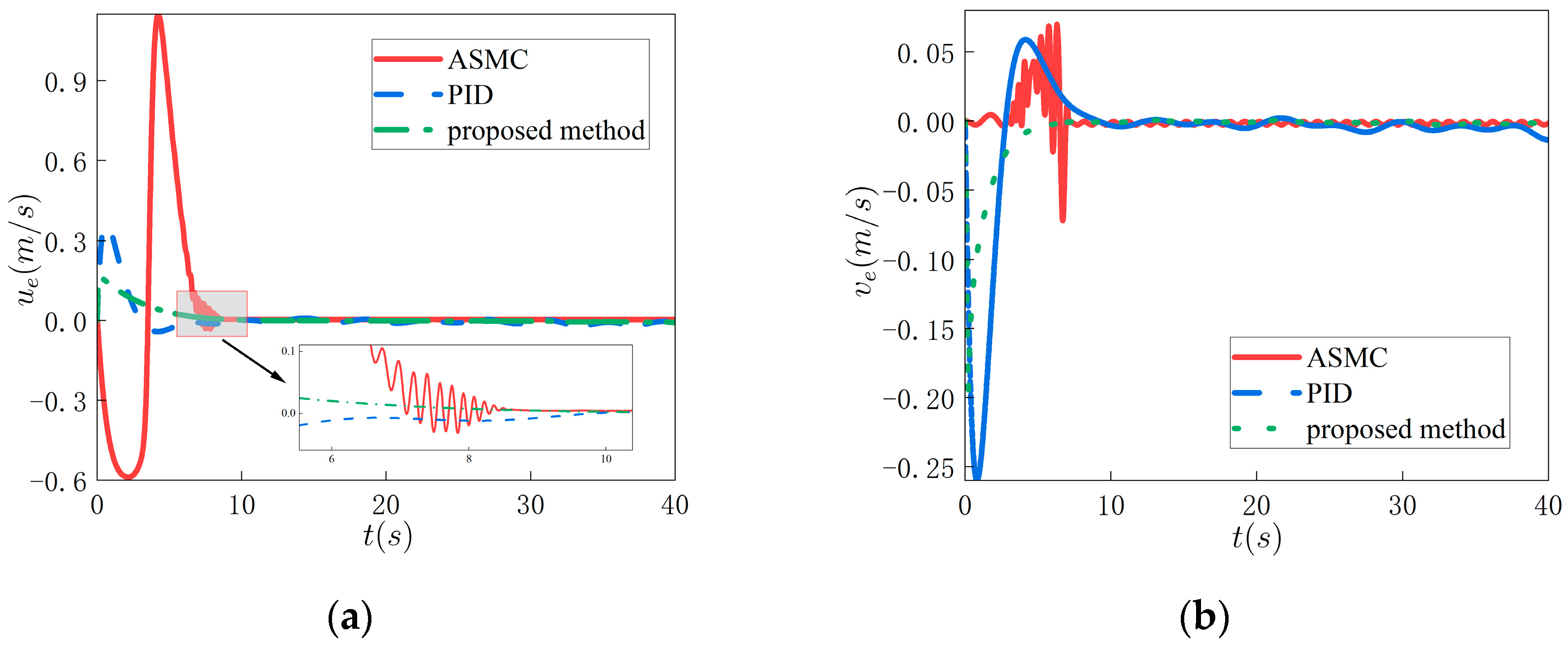
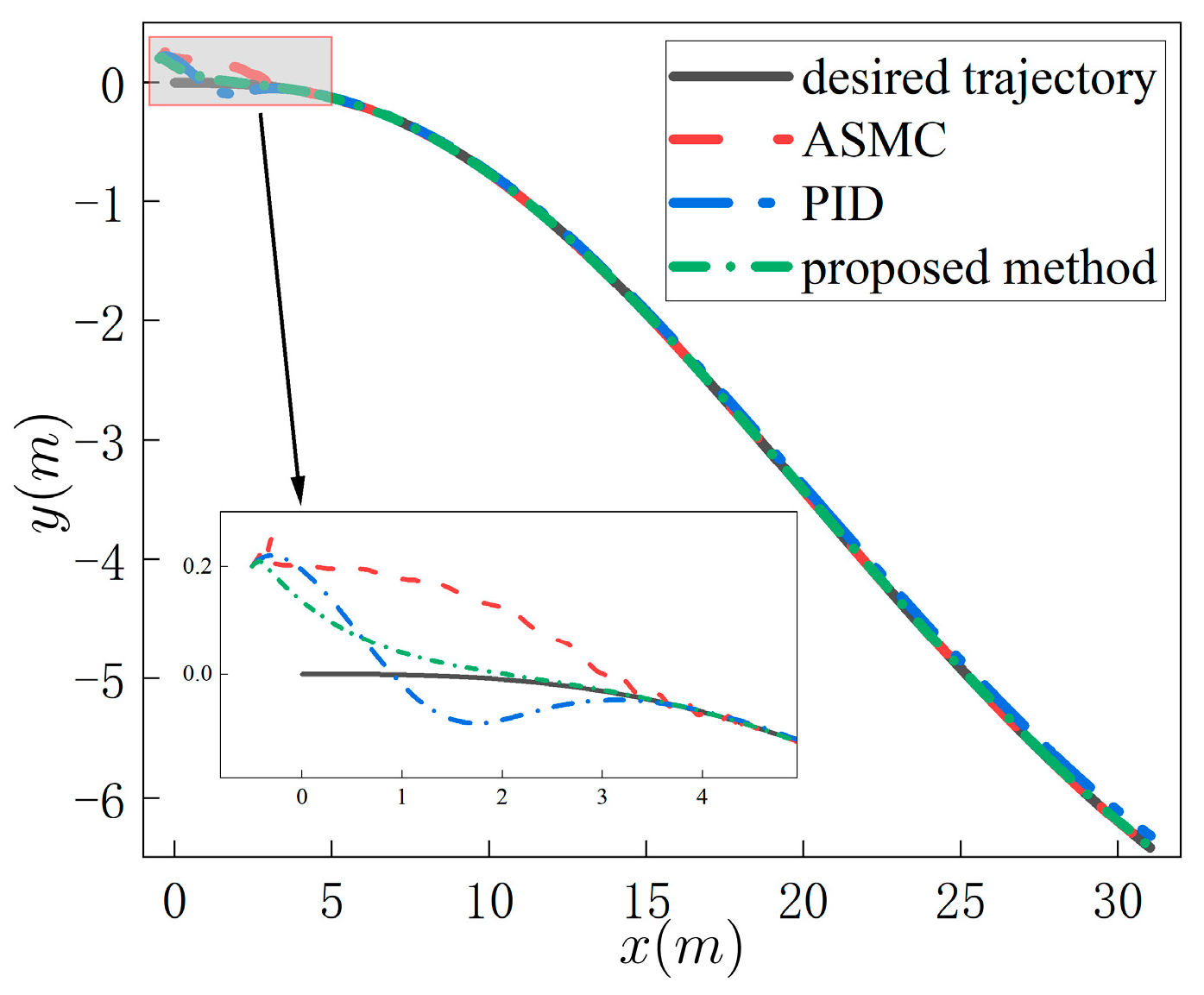
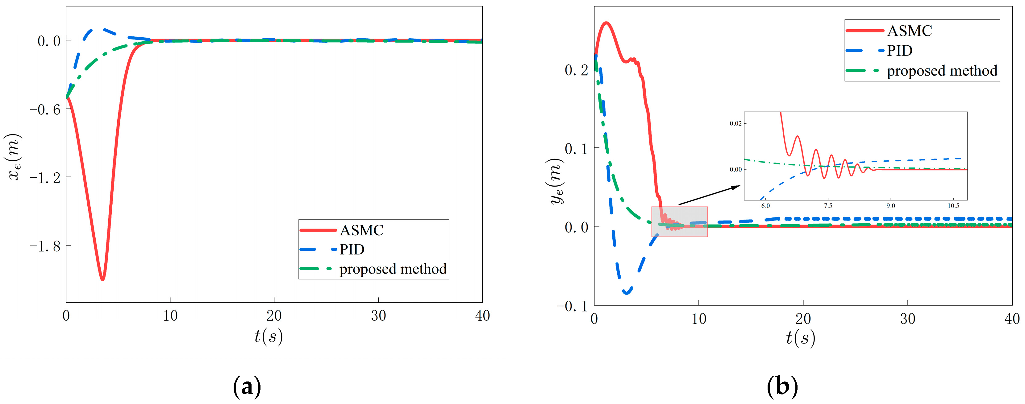
4.2. Advantages Highlight

To provide a comprehensive evaluation of the designed control strategy and showcase its superiority, we conducted additional numerical simulations in this subsection. Specifically, we compared the performance of the designed control strategy with that of the PID controller and ASMC controller. Appendix A contains detailed descriptions of these two control schemes, including their comprehensive formulations and the selected parameters.
The desired trajectory is same as Formula (50), and the desired velocity are given by  u d = 0 t 0.01 cos 0.015 π t d t v d = 0 t 0.05 sin 0.01 π t d t , and  r d = 0 t 0.01 cos 0.002 π t d t . Here,  η 0 was set as  0.5 ,   0.2 ,   0 T , and  υ 0 = 0.5 ,   0.0 ,   0.0 T . We chose  h 1 = 0 h 2 = 0 , and  h 3 = 0 .
From Figure 8, it can be observed that the USV, under the influence of different control strategies, effectively tracked the desired trajectory with good accuracy. The USV maintained stable motion throughout the entire trajectory, accurately following the desired trajectory.
From Figure 9a,b, it is evident that the tracking errors under the influence of the three different controllers exhibited distinct characteristics. Specifically, under the proposed controller, the initial tracking errors were effectively maintained within a relatively small range. On the other hand, the remaining two controllers demonstrated comparatively large initial errors, this observation means that these controllers tend to output larger forces or torques during the initial stage of operation, which can potentially lead to more pronounced deviations from the desired trajectory.
Figure 10 provides the velocity tracking errors under the influence of the three different controllers. Notably, when the proposed controller was employed, the velocity error remained relatively stable, which ensured satisfactory tracking performance. However, when the PID controller was utilized, a small amount of initial overshoot was observed during the early stages, which can impact the transient response of the system. Under the influence of the ASMC controller, a certain degree of chattering was observed as the USV approached the desired trajectory. While this chattering may introduce some deviation from the desired trajectory, it is important to note that the system still exhibited an overall robustness.
Moreover, to enhance the precision and clarity of our analysis, we provide a comprehensive quantitative comparison in Table 1. It becomes evident that the proposed control algorithm demonstrates superior performance and outperforms the other considered controllers in terms of stability and tracking accuracy.

5. Conclusions

In this paper, we studied the anti-saturation prescribed performance tracking control problem of USVs subject to model uncertainties, time-varying external disturbances, and actuator saturation.
First, for the under-actuated USV, we employed a coordinate transformation-based state-extension method. By offsetting the center of gravity of the USV, we incorporated the influence of the heading angle into the tracking errors in the x- and y-directions. This offset resulted in a redefinition of the tracking errors, allowing us to use the same two control inputs to simultaneously control the position tracking errors and the heading angle without requiring additional control inputs. This method provides a concise and efficient solution for the trajectory tracking of under-actuated USVs.
Second, we addressed the trajectory tracking problem of the USV under external disturbances and saturation constraints. By combining PTPPC with the back-stepping method, we reduced the complexity of the controller design and ensured satisfactory control performance within the specified performance framework. Additionally, we achieved the desired convergence time. This integrated control strategy offers a feasible and effective solution for trajectory tracking of USVs in practical applications where disturbances and constraints are present.
However, the limitations of this study are that our research primarily focused on theoretical developments and simulation validation to demonstrate the effectiveness of our approach. Conducting experimental tests on USVs involves significant logistical challenges, but such experiments could enhance the value of our research. Therefore, future research directions could involve designing under-actuated USV controllers and conducting experimental validation, particularly in scenarios involving actuator failures. This would contribute to a more comprehensive evaluation and validation of the performance and robustness of our approach in practical applications.

Author Contributions

Conceptualization, Y.R., L.Z., and Y.Y.; software, Y.Y. and L.Z.; validation, Y.R., L.Z., and S.L.; investigation, Y.R. and Y.T.; methodology, Y.R. and L.Z.; data curation, S.L. and Y.T.; writing—original draft preparation, Y.R.; writing—review and editing, L.Z. and Y.Y.; visualization, Y.Y. and S.L. All authors have read and agreed to the published version of the manuscript.

Funding

This research was funded by Excellent Youth Foundation of Heilongjiang Province of China, grant number YQ2021E013 and The National Key Research and Development Program of China, grant number 2021YFC2803400.

Institutional Review Board Statement

Not applicable.

Informed Consent Statement

Not applicable.

Data Availability Statement

Access to the data will be considered upon request by the authors.

Conflicts of Interest

The authors declare no conflict of interest.

Appendix A

  • PID control scheme
We adopted the PID controller as one of the comparative methods; the PID controller has been extensively researched and applied in many fields, making it a common benchmark for comparison with our designed control strategy. Thus, the controller is given as follows:
τ = G 1 α 1 ζ e + α 2 0 t ζ e d t + α 3 ζ ˙ e
where  α 1 α 2 , and  α 3 are the control gains. Here, we selected  α 1 = 15 α 2 = 10 , and  α 3 = 15 .
2.
Adaptive SMC control scheme
We used the ASMC (adaptive sliding mode control) method proposed in the work [44] as one of the comparative methods in our simulation study. Regarding the parameter selection, we sought guidance from the referenced paper, which provides a detailed explanation of the parameter selection process and the underlying rationale.
The following controller is given:
τ = M R 1 u R ˙ v + C v + D v u = η d + H η ˜ ˙ k 1 k 2 e 0.1 t η ˜ ˙ H η ˜ η ˜ ˙ H η ˜
where  H k 1 , and  k 2 are the control gains. In the present case, the gains we selected as  H = d i a g 0.3 , 0.3 , 0.5 k 1 = 0.205 , and  k 2 = 1.205 .

References

  1. Abrougui, H.; Nejim, S.; Hachicha, S.; Zaoui, C.; Dallagi, H. Modeling, parameter identification, guidance and control of an unmanned surface vehicle with experimental results. Ocean Eng. 2021, 241, 110038. [Google Scholar] [CrossRef]
  2. Liu, Z.; Zhang, Y.; Yu, X.; Yuan, C. Unmanned surface vehicles: An overview of developments and challenges. Annu. Rev. Control 2016, 41, 71–93. [Google Scholar] [CrossRef]
  3. Manley, J.E. Unmanned Maritime Vehicles, 20 years of commercial and technical evolution. In Proceedings of the OCEANS 2016 MTS/IEEE Monterey, Monterey, CA, USA, 19–23 September 2016; pp. 1–6. [Google Scholar]
  4. Zhu, C.; Huang, B.; Lu, Y.; Li, X.; Su, Y. Distributed Affine Formation Maneuver Control of Autonomous Surface Vehicles With Event-Triggered Data Transmission Mechanism. IEEE Trans. Control Syst. Technol. 2023, 31, 1006–1017. [Google Scholar] [CrossRef]
  5. Chen, D.; Zhang, J.; Li, Z. A Novel Fixed-Time Trajectory Tracking Strategy of Unmanned Surface Vessel Based on the Fractional Sliding Mode Control Method. Electronics 2022, 11, 726. [Google Scholar] [CrossRef]
  6. Chen, X.; Zhou, D.; Liu, Z.; Zhang, J.; Wang, L. Adaptive sliding-mode trajectory tracking control of underactuated unmanned surface vessels. Guofang Keji Daxue Xuebao/J. Natl. Univ. Def. Technol. 2018, 40, 127–134. [Google Scholar] [CrossRef]
  7. Dong, J.; Zhao, M.; Cheng, M.; Wang, Y. Integral terminal sliding-mode integral backstepping adaptive control for trajectory tracking of unmanned surface vehicle. Cyber-Phys. Syst. 2023, 9, 77–96. [Google Scholar] [CrossRef]
  8. Guo, H.; Chen, M.; Jiang, Y.; Lungu, M. Distributed Adaptive Human-in-the-Loop Event-Triggered Formation Control for QUAVs With Quantized Communication. IEEE Trans. Ind. Inform. 2023, 19, 7572–7582. [Google Scholar] [CrossRef]
  9. Dong, Z.; Wan, L.; Li, Y.; Liu, T.; Zhang, G. Trajectory tracking control of underactuated USV based on modified backstepping approach. Int. J. Nav. Archit. Ocean Eng. 2015, 7, 817–832. [Google Scholar] [CrossRef]
  10. Van, M.; Do, V.-T.; Khyam, M.O.; Do, X.P. Tracking control of uncertain surface vessels with global finite-time convergence. Ocean Eng. 2021, 241, 109974. [Google Scholar] [CrossRef]
  11. Bechlioulis, C.P.; Rovithakis, G.A. Robust Adaptive Control of Feedback Linearizable MIMO Nonlinear Systems With Prescribed Performance. IEEE Trans. Autom. Control. 2008, 53, 2090–2099. [Google Scholar] [CrossRef]
  12. Elhaki, O.; Shojaei, K. Neural network-based target tracking control of underactuated autonomous underwater vehicles with a prescribed performance. Ocean Eng. 2018, 167, 239–256. [Google Scholar] [CrossRef]
  13. Guo, Z.; Oliveira, T.R.; Guo, J.; Wang, Z. Performance-Guaranteed Adaptive Asymptotic Tracking for Nonlinear Systems With Unknown Sign-Switching Control Direction. IEEE Trans. Autom. Control 2023, 68, 1077–1084. [Google Scholar] [CrossRef]
  14. Yuhan, Z.; Kun, W.; Wei, S.; Zhou, L.; Zhongzhong, Z.; Hao, J.G. Back-Stepping Formation Control of Unmanned Surface Vehicles With Input Saturation Based on Adaptive Super-Twisting Algorithm. IEEE Access 2022, 10, 114885–114896. [Google Scholar] [CrossRef]
  15. Li, J.; Xiang, X.; Dong, D.; Yang, S. Saturated-command-deviation based finite-time adaptive control for dynamic positioning of USV with prescribed performance. Ocean Eng. 2022, 266, 112941. [Google Scholar] [CrossRef]
  16. Chen, B.; Tan, L. Adaptive Anti-saturation Tracking Control with Prescribed Performance for Hypersonic Vehicle. Int. J. Control Autom. Syst. 2020, 18, 394–404. [Google Scholar] [CrossRef]
  17. Ik Han, S.; Lee, J. Finite-time sliding surface constrained control for a robot manipulator with an unknown dead-zone and disturbance. ISA Trans. 2016, 65, 307–318. [Google Scholar] [CrossRef] [PubMed]
  18. Wu, X.; Zheng, W.; Zhou, X.; Shao, S. Adaptive dynamic surface and sliding mode tracking control for uncertain QUAV with time-varying load and appointed-time prescribed performance. J. Frankl. Inst. 2021, 358, 4178–4208. [Google Scholar] [CrossRef]
  19. Fan, Y.; Jing, W.; Bernelli-Zazzera, F. Nonlinear Tracking Differentiator Based Prescribed Performance Control for Space Manipulator. Int. J. Control Autom. Syst. 2023, 21, 876–889. [Google Scholar] [CrossRef]
  20. Zhu, C.; Zhang, E.; Li, J.; Huang, B.; Su, Y. Approximation-free appointed-time tracking control for marine surface vessel with actuator faults and input saturation. Ocean Eng. 2022, 245, 110468. [Google Scholar] [CrossRef]
  21. Mishra, P.K.; Jagtap, P. Approximation-Free Prescribed Performance Control With Prescribed Input Constraints. IEEE Control Syst. Lett. 2023, 7, 1261–1266. [Google Scholar] [CrossRef]
  22. Wu, Y.; Li, B.; Du, H.; Zhang, N.; Zhang, B. Fault-tolerant prescribed performance control of active suspension based on approximation-free method. Veh. Syst. Dyn. 2022, 60, 1642–1667. [Google Scholar] [CrossRef]
  23. Cao, G.; Yang, J.; Qiao, L.; Yang, Z.; Zhang, W. Adaptive output feedback super twisting algorithm for trajectory tracking control of USVs with saturated constraints. Ocean Eng. 2022, 259, 111507. [Google Scholar] [CrossRef]
  24. Qin, H.; Li, C.; Sun, Y. Adaptive neural network-based fault-tolerant trajectory-tracking control of unmanned surface vessels with input saturation and error constraints. IET Intell. Transp. Syst. 2020, 14, 356–363. [Google Scholar] [CrossRef]
  25. Trakas, P.S.; Bechlioulis, C.P. Robust Adaptive Prescribed Performance Control for Unknown Nonlinear Systems with Input Amplitude and Rate Constraints. IEEE Control. Syst. Lett. 2023, 7, 1801–1806. [Google Scholar] [CrossRef]
  26. Guo, G.; Zhang, P. Asymptotic Stabilization of USVs with Actuator Dead-Zones and Yaw Constraints Based on Fixed-Time Disturbance Observer. IEEE Trans. Veh. Technol. 2020, 69, 302–316. [Google Scholar] [CrossRef]
  27. Deng, Y.; Zhang, X.; Im, N.; Zhang, G.; Zhang, Q. Adaptive fuzzy tracking control for underactuated surface vessels with unmodeled dynamics and input saturation. ISA Trans. 2020, 103, 52–62. [Google Scholar] [CrossRef] [PubMed]
  28. Xiaodong, S.; Qinglei, H.; Yang, S.; Boyan, J. Fault-Tolerant Prescribed Performance Attitude Tracking Control for Spacecraft Under Input Saturation. IEEE Trans. Control Syst. Technol. 2020, 28, 574–582. [Google Scholar] [CrossRef]
  29. Rodrigues, V.H.P.; Hsu, L.; Oliveira, T.R.; Fridman, L. Adaptive sliding mode control with guaranteed performance based on monitoring and barrier functions. Int. J. Adapt. Control Signal Process. 2022, 36, 1252–1271. [Google Scholar] [CrossRef]
  30. Li, L.; Dong, K.; Guo, G. Trajectory tracking control of underactuated surface vessel with full state constraints. Asian J. Control. 2021, 23, 1762–1771. [Google Scholar] [CrossRef]
  31. Alvaro-Mendoza, E.; Gonzalez-Garcia, A.; Castaneda, H.; De Leon-Morales, J. Novel adaptive law for super-twisting controller: USV tracking control under disturbances. ISA Trans. 2023, 139, 561–573. [Google Scholar] [CrossRef]
  32. Fan, Y.; Qiu, B.; Liu, L.; Yang, Y. Global fixed-time trajectory tracking control of underactuated USV based on fixed-time extended state observer. ISA Trans. 2023, 132, 267–277. [Google Scholar] [CrossRef] [PubMed]
  33. Wu, G.X.; Ding, Y.; Tahsin, T.; Atilla, I. Adaptive neural network and extended state observer-based non-singular terminal sliding mode tracking control for an underactuated USV with unknown uncertainties. Appl. Ocean Res. 2023, 135, 103560. [Google Scholar] [CrossRef]
  34. Lv, C.; Yu, H.; Chen, J.; Zhao, N.; Chi, J. Trajectory tracking control for unmanned surface vessel with input saturation and disturbances via robust state error IDA-PBC approach. J. Frankl. Inst. 2022, 359, 1899–1924. [Google Scholar] [CrossRef]
  35. Ashrafiuon, H.; Muske, K.; McNinch, L.; Soltan, R. Sliding-Mode Tracking Control of Surface Vessels. Ind. Electron. IEEE Trans. 2008, 55, 4004–4012. [Google Scholar] [CrossRef]
  36. Zhang, L.; Zheng, Y.; Huang, B.; Su, Y. Finite-time trajectory tracking control for under-actuated unmanned surface vessels with saturation constraint. Ocean Eng. 2022, 249, 110745. [Google Scholar] [CrossRef]
  37. Lamraoui, H.C.; Qidan, Z.; Bouzid, Y. Improved active disturbance rejecter control for trajectory tracking of unmanned surface vessel. Mar. Syst. Ocean Technol. 2022, 17, 18–26. [Google Scholar] [CrossRef]
  38. Yao, Q.; Jahanshahi, H.; Liu, C.; Alotaibi, A.; Alsubaie, H. Disturbance Attenuation Trajectory Tracking Control of Unmanned Surface Vessel Subject to Measurement Biases. Axioms 2023, 12, 361. [Google Scholar] [CrossRef]
  39. Shan, Q.; Wang, X.; Li, T.; Chen, C.L.P. Finite-time control for USV path tracking under input saturation with random disturbances. Appl. Ocean Res. 2023, 138, 103628. [Google Scholar] [CrossRef]
  40. Mousavi, S.H.; Khayatian, A. Dead Zone Model Based Adaptive Backstepping Control for a Class of Uncertain Saturated Systems. IFAC Proc. Vol. 2011, 44, 14489–14494. [Google Scholar] [CrossRef]
  41. Sun, R.; Na, J.; Zhu, B. Robust approximation-free prescribed performance control for nonlinear systems and its application. Int. J. Syst. Sci. 2018, 49, 511–522. [Google Scholar] [CrossRef]
  42. Ding, Z.; Wang, H.; Sun, Y.; Qin, H. Adaptive prescribed performance second-order sliding mode tracking control of autonomous underwater vehicle using neural network-based disturbance observer. Ocean Eng. 2022, 260, 111939. [Google Scholar] [CrossRef]
  43. Bechlioulis, C.P.; Rovithakis, G.A. A low-complexity global approximation-free control scheme with prescribed performance for unknown pure feedback systems. Automatica 2014, 50, 1217–1226. [Google Scholar] [CrossRef]
  44. Hsu, L.; Oliveira, T.R.; Cunha, J.P.V.S.d.; Yan, L. Adaptive unit vector control of multivariable systems using monitoring functions. Int. J. Robust Nonlinear Control 2018, 29, 583–600. [Google Scholar] [CrossRef]
Figure 1. Position of USV in two coordinates.
Jmse 11 01717 g001
Figure 2. Comparison of two saturation constraints by using corresponding models. (Plot the condition of  τ c i = 5 sin 1.5 t ,   α i = 10 ,   χ i = 0.16 ).
Jmse 11 01717 g002
Figure 3. Diagram of the proposed control architecture.
Jmse 11 01717 g003
Figure 4. Trajectory tracking under three different disturbances.
Jmse 11 01717 g004
Figure 5. Position tracking errors ((a) the tracking error in the x direction and (b) the tracking error in the y direction).
Jmse 11 01717 g005
Figure 6. Velocity tracking errors ((a) the surge speed error  u e and (b) the sway speed error  v e ).
Jmse 11 01717 g006
Figure 7. Time evolution of control inputs under three different disturbances ((a) the control force  τ u and (b) the control torque  τ r ).
Jmse 11 01717 g007
Figure 8. Time responses of position trajectory.
Jmse 11 01717 g008
Figure 9. Position tracking errors ((a) the tracking error along X axis  x e and (b) the tracking error along Y axis    y e ).
Jmse 11 01717 g009
Figure 10. Velocities tracking errors ((a) the surge speed  u and (b) the sway speed  v ).
Jmse 11 01717 g010
Table 1. Quantitative Analysis of Tracking Error (RMSE).
Control SchemeSteady-State Error
  x e   y e   u e   v e
Proposed method0.00310.00320.00250.0026
ASMC0.00350.00370.00310.0032
PID0.00400.00400.00270.0031
Disclaimer/Publisher’s Note: The statements, opinions and data contained in all publications are solely those of the individual author(s) and contributor(s) and not of MDPI and/or the editor(s). MDPI and/or the editor(s) disclaim responsibility for any injury to people or property resulting from any ideas, methods, instructions or products referred to in the content.

