Dynamic Response Analysis of Submarines Based on FEM-ALE Coupling Method in Floating Ice Conditions

Abstract

To address global challenges, research on the safety of polar navigation is indispensable. However, most of studies focus on traditional surface vessels, with few research studies on submarine. The dynamic response of submarine during surface navigation in floating ice channels under special conditions is studied in this work. Firstly, a model of the submarine incorporating an intact internal frame was established. Subsequently, the FEM-ALE coupled method was employed to simulate the structure-ice interaction, and the obtained results was verified by the Colbourne method. Then, the parametric study (navigation speed, ice thickness, and floating ice size) were analyzed from the perspectives of ice resistance, stress and plastic strain. Finally, an empirical equation suitable for the interaction between submarine and floating ice during surface navigation is improved based on the Colbourne method.

1. Introduction

With the increasing degree of globalization and the ever-growing energy shortage problem, the Arctic region harbors paramount developmental significance [1]. The Arctic region has a transcontinental route linking Asia and Europe, and it contains a large amount of untapped resources [2]. However, numerous natural obstacles, such as floating ice, layer ice, and ridges, as well as extreme environmental conditions, pose a serious threat to the safety of polar navigation. Therefore, safety assessments of structures such as icebreakers, commercial vessels, and submarines that navigate in the Arctic region are particularly important [3]. Current researches mainly focuses on traditional surface vessels, such as icebreakers and commercial vessels, with limited research on submarines.

The dynamic response during ship-ice interaction process is affected by the shape of the ship, structural strength, and ice properties [4]. Analytical methods that are conventional have difficulty comprehensively considering multiple factors. Therefore, researchers commonly use empirical equation methods, simulation methods, and experimental methods. The experimental method can be divided into full-scale ship tests and model tests, which yield more accurate results but are costly and time consuming. Empirical equations are derived from the summary and integration of data from considerable of tests, and often apply only to a certain type of operating condition. A relatively lower cost is associated with the simulation method, rendering it applicable to a majority of operational conditions [5].

In the early nineteenth century, experimental methods were primarily employed for the accumulation of a significant volume of crucial data, from which empirical equations were derived. The earliest ice resistance equation, presented by Runeberg [6], took into consideration the influences of frictional forces and bow trim angles. Ship design parameters were initially considered by Shimanskii [7], while Kashteljan [8] pioneered the partitioning of ice resistance into breaking resistance, overturning and submergence resistance, and damaged floating ice resistance. Jones [9] introduced semi-empirical methods into the study of continuous ice breaking. Based on the aforementioned research and the accumulation of a substantial amount of data, numerous empirical equations with notable effectiveness were developed. For level ice conditions, methods such as the Lindqvist [10] approach, which incorporated considerations of friction and ship hull geometry, as well as the Riska [11] method derived from the modified Lindqvist approach, had been established. Conversely, for floating ice conditions, the relevant empirical equations were predominantly compiled and summarized from experimental data. Examples include the Bronnikov method [12] based on ship tests and the Mellor method based on the Mohr-Coulomb failure criterion [13].

In the experimental aspect, Daley [14] conducted observations on the failure process of the ice layer through full-scale and model-scale experiments and proposed a contact model for the ice layer’s edge. Jeong [15] conducted ice tank experiments with square-shaped floating ice in three different channel widths and analyzed the impact of ice size on resistance, while proposing a rapid method for calculating ice concentration. Kim [16] conducted model-scale ice resistance experiments in a simulated ice environment using triangular ice elements made of paraffin instead of real ice. Several operating conditions were set based on different velocities, ice concentration, and ship hull waterline entry angles. The experimental results were compared with numerical simulation results. Jeong [17] and others conducted model-scale ship tests in a frozen ice region at the MOERI ice tank, resulting in the prediction of planar ice resistance for various thicknesses and bending strengths.

With the advancement of computer technology and numerical simulation methods, researchers have begun to employ simulation techniques to study the physical processes and mechanical characteristics of ice collisions. Among these, FEM, SPH, DEM, and their combined usage are the most common research approaches employed today.

The application of the FEM to simulate ice loads was pioneered by Määttänen and Hoikkanen in 1990, while Evgin et al. subsequently successfully utilized the DEM for icebreaking simulations [18]. Munjiza [19] proposed the FEM-DEM method, which integrated the advantages of both approaches, using FEM to simulate ice fracture and DEM to simulate ice accumulation. Huang et al. [20] based on the combination of CFD and DEM methods, investigated fragmented ice channels and discovered a linear relationship between the thickness and diameter of floating ice and ice resistance. Based on the ice shell collision mechanism and fundamental icebreaking characteristics, Karl [21] introduced a simplified numerical model to predict the ice impact forces acting on the vessel under horizontal ice conditions. The model addresses two critical failure modes, namely local crushing and flexural fracture. Andrei [22] constructed a CFD numerical model based on the DEM-BEM theory, suitable for simulating the interaction between floating structures and fragmented ice. The potential flow theory was employed to predict the flow field around the ship hull and the surrounding fragmented ice. Finally, the computational results were compared with the ice tank test results.

Zhang [23] performed numerical simulations of the collision between a vertical cylindrical structure and layered ice by utilizing LS-DYNA finite element software. Two different thicknesses of cohesive element ice models were constructed, and the S-ALE fluid–structure coupling method was employed. Song, Kim, and others [24] utilized the ALE method within the LS-DYNA finite element software to simulate the mutual interaction between floating ice and marine structures. They accounted for the fluid–structure interaction problem and validated the correctness of the ALE method and the coupling algorithm in the interaction between fluid, ice, and structures.

Apart from those, Su [25] incorporated numerical models to investigate the overall and local ice loads on ship structures. Through two case studies, simulated ice loads on the vessel were examined, analyzing ship performance, statistical framework loads induced by ice, and the spatial distribution of ice loads around the ship. A comparison with field measurements was conducted as well. Chai [26] applied probability methods and models to seek the correlation between ice-induced load statistics and major ice conditions in the field of ship and ocean engineering. Zhao [27] performed the probability-based fatigue damage assessment of vessels traversing horizontal ice fields. A novel procedure utilizing numerical simulation had been developed for the evaluation of fatigue damage, and the process was demonstrated through a hypothetical scenario involving the icebreaking vessel Snow Dragon 2. The sensitivity of the procedure to key analysis parameters, such as sample size and initial crack size, was also taken into consideration by Zhao [28]. The impact of low temperature on the computational results was analyzed as well.

The icebreaking research mentioned above primarily focuses on surface vessels, with limited experimental studies and insufficient available data conducted on submarines, thus few related empirical equations have been proposed for the ice resistance of submarines. However, they may encounter collisions with small-scale floating ice when they need to surface during certain special emergency tasks. This paper aims to investigate the dynamic response of submarines navigating through the surface of floating ice-field using the FEM-ALE coupling approach. The effects of navigation speed, ice thickness, and floating ice size on the polar navigation safety of submarines are studied. Special emphasis is placed on the ice resistance force-time history, as well as the stress–strain distribution on both the surface and interior of the structures, to propose a reference condition for safe navigation. The novelty of this study lies in the fact that the submarines are not modeled as empty shells, but as fully integrated bow structures with internal plates, frames, and trusses. Based on the numerical results, critical conditions and empirical equations are proposed.

2. Theoretical Background

2.1. The Theory of Ship-Ice Interaction

The collision between ships and ice involves a significant amount of non-linear behaviors, such as material non-linearity, geometric non-linearity, and contact non-linearity. Material non-linearity refers to the complex stress–strain relationship of sea ice material, which is influenced by multiple factors. Geometric non-linearity refers to the large deformation of sea ice, which is not suitable for the small deformation principle. Contact non-linearity refers to the unstable contact between two substances, resulting in a large number of non-linear changes. In this work, comprehensive consideration is given to the three non-linearities, where both the sea ice and structure are simplified as elastic-plastic materials, and the contact is computed using an automatic face-to-face contact algorithm. In terms of the algorithm, the simulation calculation of the ship collision process essentially involves the numerical solution of collision equations, which is accomplished using the explicit central difference method [29].

When the results of 0, …, $t_n$, time steps are known:

$$M\stackrel{··}{U}(t_n)=P(t_n)-F^{\mathrm{int}}(t_n)+H(t_n)-C\stackrel{·}{U}(t_n)$$

(1)

where: $P(t)$—external force vector;

$F^{\mathrm{int}}(t_n)$—internal force vector;

$F^{\mathrm{int}}(t_n)={\displaystyle \sum {\displaystyle \underset{\Omega }{\int }{B}^T{\sigma }_{n}d\Omega +F^{contact}}}$, Nodal element internal force;

$H(t_n)$—hourglass resistance.

Inverting the equation, it can get:

$$\stackrel{··}{U}(t_n)=M^{-1}[P(t_n)-F^{\mathrm{int}}(t_n)+H(t_n)-C\stackrel{·}{U}(t_n)]$$

(2)

According to the definition of finite difference method, the displacement, velocity, and acceleration at time $t_{n+1}$ can be solved by the following equation:

$$\stackrel{·}{U}(t_{n+\frac{1}{2}})=\stackrel{·}{U}(t_{n-\frac{1}{2}})+\stackrel{··}{U}(t_n)\mathsf{\Delta }{t}_n$$

(3)

$$U\left(t_{n+1}\right)=U\left(t_n\right)+\stackrel{·}{U}(t_{n+\frac{1}{2}})\mathsf{\Delta }{t}_{n+\frac{1}{2}}$$

(4)

where: $\mathsf{\Delta }{t}_{n+\frac{1}{2}}=\frac{\mathsf{\Delta }{t}_n+\mathsf{\Delta }{t}_{n+1}}{2}$, $\mathsf{\Delta }{t}_{n-\frac{1}{2}}=\frac{\mathsf{\Delta }{t}_n+\mathsf{\Delta }{t}_{n-1}}{2}$.

After a series of calculations, the mass influence coefficients are transformed into a diagonal matrix, achieve decoupling, and enable independent computations. In this calculation process, the influence of the stiffness matrix is assumed to be neglected, and only the central single-point integration is considered, significantly reducing the computational steps and decreasing computation time.

2.2. The Material Model

Sea ice is a typical nonlinear material whose physical properties are influenced by various factors, including load strain, temperature, ice age, and salinity. Describing the constitutive model of sea ice accurately in simulation calculations is challenging, and existing research often replaces sea ice materials with ice load models.

At present, there is no perfect ice material model due to the complex physical properties and microstructure of ice. Based on experimental and simulation results, researcher [30] have proposed several reliable ice load models, including elasto-plastic models based on plasticity theory, viscoplastic models, improved models, anisotropic failure models, and visco-elastic-plastic models based on the particle flow theory of sea ice, as well as crushable foam models.

For the elastic-plastic model [31], it is assumed that the material undergoes only elastic deformation when the stress is relatively low. However, when the stress exceeds the yield stress, the stress–strain curve deviates from the elastic stage and becomes a sloping line. Once the yield stage is reached, the material starts exhibiting irreversible plastic deformation, and as the stress continues to increase, the material may fail and undergo damage.

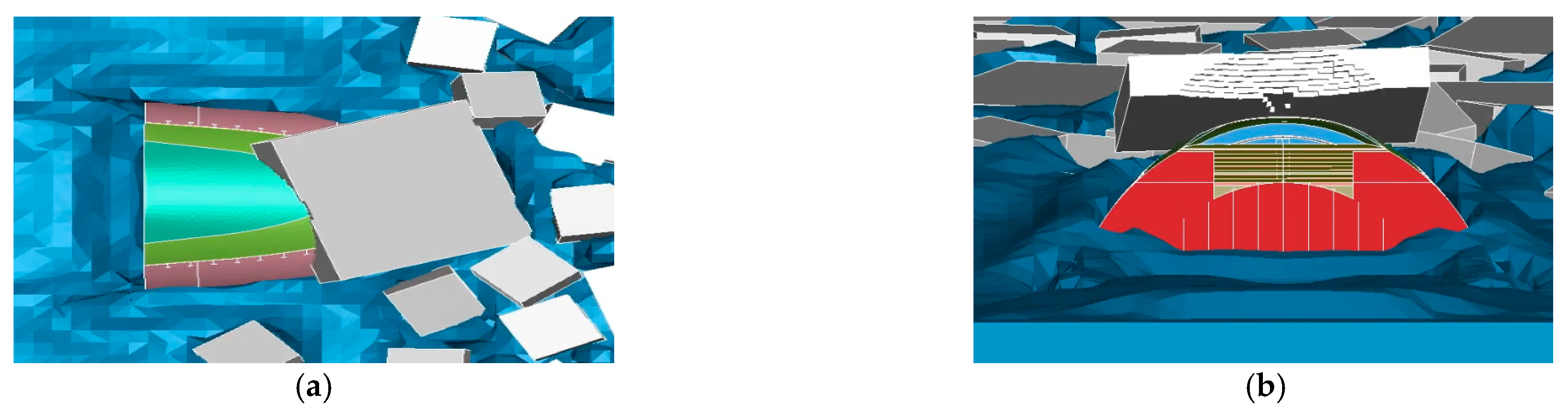
Based on the existing experiments, the stress-strain curve of ice floe is shown in red line in Figure 1. However, elastoplastic models are often used instead of actual ice floes in the simulation of structure-ice interaction. The curve is approximated as two straight lines, the former part is the elastic stage, and the latter part is the plastic stage. The failure modes of sea ice can be simplified into four types: local fragmentation caused by compression failure, instability caused by buckling failure, cracks generated by shear failure, and fractures caused by bending failure. This study focuses on maximum floating ice sizes of only 6 m × 6 m, which are relatively small and rarely experience the latter three failure modes. Typically, only compression failure occurs, specifically in the parts directly in contact with the structure. In this work, the elastic-plastic model is utilized, which effectively captures most properties of the floating ice and enables failure simulation through mesh removal.

2.3. FEM-ALE Coupling Method

Finite element method includes Lagrangian, Eulerian, and ALE methods [32]. In the Lagrangian method, element points are identical to material points, and the element is fixed to the object, moving along with the model nodes. In the Eulerian method, element points are spatial points, and the element is fixed in space, unaffected by the movement of material points. In the ALE description, a reference configuration independent of the actual and initial configurations is introduced, with element points as reference points. The motion of the element in space is arbitrary, independent of the Lagrangian and Eulerian coordinate systems, and can be chosen as needed. When the element motion velocity is reasonable, this method can accurately simulate object deformation and track object motion, making it suitable for modeling nonlinear and large deformation changes, particularly in fluid domains. As shown in Figure 2, A, B and C are grid movements of Lagrangian, Euler, and ALE methods respectively.

In the traditional Eulerian conservation equations, the conventional terms have been replaced by relative velocity yielding the conservation equations in an arbitrary Lagrangian form, as expressed below [33]:

Mass conservation equation:

$$\frac{\partial \rho }{\partial t}\left|{}_x\right.+c·\nabla \rho =-\rho \nabla ·v$$

(5)

Momentum conservation equation:

$$\rho \left(\frac{\partial \rho }{\partial t}\left|{}_x\right.+\left(c·\nabla \right)\nu \right)=\nabla ·\sigma +\rho b$$

(6)

Energy conservation equation:

$$\rho \left(\frac{\partial \rho }{\partial t}\left|{}_x\right.+c·\nabla E\right)=\nabla ·(\sigma ·v)+v·\rho b$$

(7)

Internal energy conservation equation:

$$\rho \left(\frac{\partial \rho }{\partial t}\left|{}_x\right.+c·\nabla e\right)=\sigma ·{\nabla }^S\nu$$

(8)

At each computational instant, two distinct stages are encompassed. In the first stage, material does not flow across the boundaries of the grid, and there is no material overflow throughout the entire calculation process, ensuring mass conservation. In the second stage, material flows across the edges of the elements, referred to as convection. The ALE method computes the transport quantities, internal energy, and momentum of the various physical properties as the material passes through the element boundaries. Unlike the first stage of the Lagrangian method, the second stage involves the generation of an independent motion in the grid, separate from the material. The grid’s independent relative motion allows it to return to its original position or any other position that facilitates more accurate calculations. ALE does not support implicit time integration, dynamic relaxation, and contact. However, large deformation motion can be well described by ALE, which is applicable for fluid–structure interaction in fluid dynamics.

The main models in this work includes the submarine, floating ice, and fluid domains, with defined contacts between floating ice and the submarine, and coupling between each model and the fluid domain. Both floating ice and structures use an elastoplastic material model, representing contact between structures and floating ice as contact between elastic bodies. A penalty function algorithm is employed for contact, which checks if nodes penetrate the master surface at each time step and applies a large interface contact force at the penetrated locations. The magnitude of this force is proportional to the penetration depth and the stiffness of the master surface, ensuring high efficiency and applicability.

The collision between the ship and ice in this work is highly complex and involves erosion double-sided contact, where the structure and floating ice act as master and slave surfaces, respectively [34]. The fluid–structure interaction utilizes a penalty function algorithm, and the ALE moving mesh method is employed to calculate fluid motion. Due to the LS-DYNA explicit integration scheme utilizing the central difference method, the accuracy of calculations is affected by the hourglass deformation of quadrilateral meshes. For fluids, hourglass control based on a viscous equation is applied to suppress hourglass deformation, while for solids, hourglass control based on a stiffness equation is used to counteract hourglass deformation by deforming in the opposite direction.

2.4. Colbourne Method

The maximum ice resistance is often employed for evaluating structural strength, whereas the average ice resistance is generally utilized for calculating economic benefits. The validation of the maximum ice resistance results is carried out in this work. The Colbourne method [35], which treats the ice resistance as a unified entity by disregarding infrequent ice fracture occurrences, is adopted to validate the predicted maximum ice resistance based on the numerical simulation. This approximation aligns with the simulation settings in the computational software. According to Colbourne method the total resistance is divided into open water resistance and ice resistance, as expressed by the following equation:

$$\begin{array}{l}{R}_{OW}=C_{OW}{V}^2\\ R_P=C_P{\rho }_{i}gB{h}_i{V}^2{C}^n\end{array}$$

(9)

where:

$C_{OW}$—the open water resistance coefficient,

$C_P$—the drag coefficient of ice floe,

${\rho }_i$—the density of ice,

$h_i$—the ice thickness,

$g$—the acceleration of gravity,

$V$—the ship speed,

$C$—the concentration of ice floe.

The drag coefficient of floating ice is a dimensionless value, defined as follows:

$$C_P=\frac{R_P}{{\rho }_{i}gB{h}_i{V}^2{C}^n}$$

(10)

where:

B—maximum beam for the structure

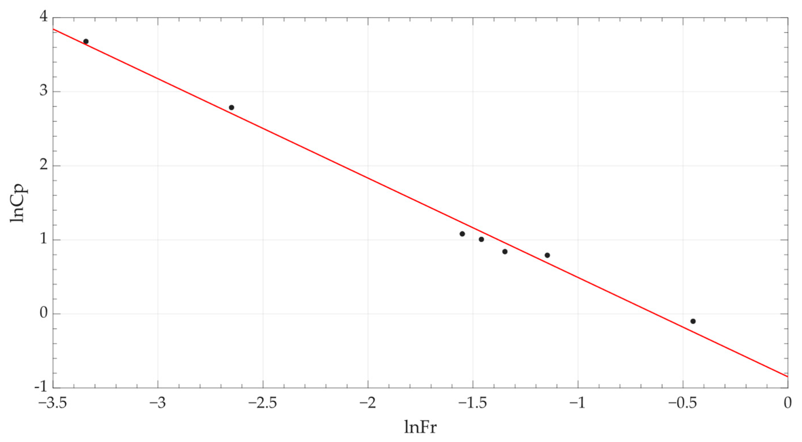
Similarly, the non-dimensionalization of navigation speed is also performed in the Colbourne method. It is considered that the Froude number is related to the ice concentration. The ice Froude number is defined as follows:

$$F{r}_P=\frac{V}{\sqrt{g{h}_{i}C}}$$

(11)

Based on the Colbourne method, it is considered that there exists a linear relationship between the natural logarithm of Cp and the natural logarithm of Fr_p. However, in the case of this study, the structure is unique and lacks relevant experimental data for validation. Therefore, utilizing multiple simulated data obtained from our own simulations, the natural logarithm of Cp and the natural logarithm of Fr_p are calculated, and a corresponding curve can be plotted. The study aims to evaluate the accuracy by inversely verifying the error in the resistance results based on this curve.

3. The Interaction between Submarine and Floating Ice

3.1. The Numerical Setup

A typical submarine is chosen for the structure-ice interaction in this work. To simplify the computational process and ensure accuracy, only the bow part which includes an internally intact plate-frame structure, is utilized for collision analysis, The length of the bow of the structure is 9.2 m, the width is 7.8 m, the height above water is 2.1 m, and the height below water is 6.7 m.

The collision between the structure and the floating ice primarily occurs with the first ice floe. To reduce computational time while maintaining accuracy, the mesh size of the first ice floe is refined to 0.1 m × 0.1 m × 0.1 m, while the remaining ice floes have a mesh size of 0.2 m × 0.2 m × 0.2 m. The ice concentration is set at 50%, and several rectangular ice floes with cross-sectional dimensions of 6 m × 6 m, 4 m × 4 m, and 2 m × 2 m are considered. The structure-ice interaction model and the investigated operating conditions are presented in Figure 3 and

Table 1. Working condition parameter.

No.	Speed (kn)	Ice Thickness (m)	The Size of the First Floating Ice (m × m)
1	6	1.2	6 × 6
2	4	1.2	6 × 6
3	2	1.2	6 × 6
4	1	1.2	6 × 6
5	6	1.0	6 × 6
6	6	0.8	6 × 6
7	6	0.5	6 × 6
8	6	1.2	4 × 4
9	6	1.2	2 × 2

, respectively.

3.2. The Material Parameters

3.2.1. The Fluid Domain

The fluid domain (sea water and air) adopts the null hydrodynamic material type in LS DYNA. The related parameters are given in

Table 2. The material parameters for the fluid domain.

	Density (kg/m3)	Cut off Pressure (Pa)	Viscosity Coefficient (Pa·s)
Sea water	1.03	−1000	1.79 × 10−3
Air	1018	−100	1.75 × 10−5

.

The effects of seawater on the behavior of the ship and ice can be considered by application of the ALE method. In LS-DYNA, the computation of fluids necessitates the definition of materials and EOS. An EOS such as the Gruneisen model is suggested to simulate water in the current FEM solver. The Gruneisen EOS with cubic shock velocity-particle velocity defines the pressure for a compressed material.

$$P=\frac{{\rho }_0{C}^2\mu \left[1+\left(1-\frac{{\gamma }_0}{2}\right)-\frac{\alpha }{2}{\mu }^2\right]}{{\left[1-\left(S_1-1\right)\mu -S_2\frac{{\mu }^2}{\mu +1}-S_3\frac{{\mu }^3}{{\left(\mu +1\right)}^2}\right]}^2}+\left({\gamma }_0+\alpha \mu \right)E_0$$

(12)

where:

$E$—the internal energy per initial volume,

$C$—the intercept of the ${\mu }_s-{\mu }_p$ curve (speed of sound in water),

$S_1$, $S_2$ and $S_3$—the coefficients of the slope of the ${\mu }_s-{\mu }_p$ curve,

${\gamma }_0$—the Gruneisen gamma parameter,

$\alpha$—the first-order volume correction to ${\gamma }_0$.

The seawater characteristics based on the relevant parameters are given in

Table 3. The EOS parameters for sea water.

	C	S1	S2	GAMAO	E0 (J)	V0 (m3)
Sea water	1480.000	1.920	−0.096	0.350	2.895 × 105	1.000

.

The air domain adopts the linear equation EOS, and the specific equation is shown in Equation (13). The related parameters are given in

Table 4. Table The EOS parameters for air.

	C0	C1	C4	C5	E0 (J)	V0 (m3)
Air	0.000	0.000	0.400	0.400	2.530 × 105	1.000

.

$$P=C_0+C_1\mu +C_2{\mu }^2+C_3{\mu }^3+\left(C_4+C_5\mu +C_6{\mu }^2\right)E$$

(13)

3.2.2. The Material Parameters for Submarines

In this work, an elastic-plastic model more suitable for high-strength steel is adopted which defines the structural deformation during the collision process of structures. Related material parameters are given in

Table 5. The material parameters for submarines.

Density (kg/m3)	Elastic Modulus (Pa)	Possion’s Ratio	Yield Strength (Pa)	Tangent Modulus (Pa)	SRC	SRP	Plastic Failure Strain
7850.0000	2.060 × 1011	0.300	3.900 × 108	1.180 × 109	3200	5.00	0.28

Where: SRC—Strain rate parameter C; SRP—Strain rate parameter p.

.

3.2.3. The Material Parameters for Floating Ice

The ice material employed in this work utilizes the previously mentioned isotropic elastic failure model. This model exhibits elastic deformation when subjected to low stress levels. However, plastic deformation occurs when the stress exceeds the yield strength. In the event that the plastic strain surpasses 0.002, the corresponding mesh elements are automatically deleted due to failure. The related parameters of the model are given in

Table 6. The material parameters for floating ice.

Density (kg/m3)	Tangent Modulus (Pa)	Yield Strength (Pa)	Hardening Modulus (Pa)	Plastic Failure Strain	Failure Pressure (Pa)	Bulk Modulus (Pa)
920.00	2.20 × 109	2.12 × 106	4.26 × 109	0.002	−4.00 × 106	5.26 × 109

.

3.3. The Verification for Numerical Model

3.3.1. The Verification for Pressure Gradient with Single Floating Ice

Before the numerical simulation of structure-ice interaction, it is necessary to validate the stability of the fluid pressure and the ability of a single ice floe to float stably. The air pressure validation is conducted by examining the variations in air pressure gradient and the temporal changes in air pressure at monitored nodes, as shown in Figure 4.

It can be seen from Figure 4 that the pressure gradually increases with depth, and the pressure at the nodes, showing in color lines, remains stable. A floating ice floe is placed within the region, and the results animation is observed and the time history of the ice floe’s acceleration is shown in Figure 5. As shown in Figure 5, the acceleration of the individual ice gradually stabilizes around zero, indicating floating stability.

3.3.2. The Verification for Ice Resistance

There are four different navigation speeds considered in this research, i.e., 1 knot, 2 knots, 4 knots, and 6 knots. In the numerical calculation, a 120-core parallel computation is employed, and the 1 kn working condition requires approximately 36 h. The simulation results provide ice resistance data, excluding the open water resistance. The specific data is shown in

Table 7. The numerical results based on structure-ice interaction.

Navigation Speed (kn)	1	2	4	6
Maximum ice resistance (N)	2.44 × 105	4.00 × 105	4.01 × 105	6.54 × 105

.

By substituting the average ice resistance into Equations (10) and (11), lnFr_p and lnCp can be obtained, as shown in

Table 8. lnFr_p and lnCp data.

Navigation Speed (kn)	1	2	4	6
lnCp	3.679	2.787	1.403	1.081
lnFrp	−1.551	−0.858	−0.165	0.241

.

The relation between Fr_p and lnCp is presented in Figure 6. Based on the least squares method, the trendline equation is derived as lnCp= −1.526lnFr_p + 1.3474. Applying the operating conditions of a velocity of 6 knots, ice thickness of 1.2 m, and the dimensions of the initial ice floe as 6 m × 6 m, the ice Froude number is obtained. Then, the natural logarithm of Cp is obtained. Finally, the theoretical ice resistance is calculated, resulting in a value of 5.91 × 10⁵ N. In comparison, the simulation yields a predicted resistance of 6.54 × 10⁵ N, indicating a discrepancy of 10.65%. Therefore, the obtained results are deemed reliable.

4. Results and Discussion

4.1. The Structural Response of Structure-Ice Interaction

The work conditions in the previous section are subjected to in-depth analysis. Combined with the animation and time history curve, some mechanism of submarine collisions with ice floes was discovered. Different from traditional icebreakers due to the similar size between the submarine and the ice floes, the submarine almost only collides with the first ice floe, and the remaining floes are pushed aside without accumulating. Following impact, the ice floe momentarily attains higher velocity than the structure due to the latter’s significantly greater mass, subsequently decelerating until the next impact occurs, as shown in Figure 7. This repetitive loading–unloading process leads to multiple peaks in the response. The location where the structure encounters collisions and the internal circular plate experience significant stress, making them susceptible to plastic deformation.

4.2. The Parametric Study of Structure-Ice Interaction

4.2.1. The Effect of Ship Speed on Structural Response

To study the effect of navigation speed on ice resistance, the ice thickness is maintained at 1.2 m, and the dimensions of the initial ice floe remain constant at 6 m × 6 m. The results are computed for velocities of 6 knots, 4 knots, 2 knots, and 1 knot, respectively. The corresponding results are shown in Figure 8 and Figure 9.

It can be seen from Figure 8 that when the structure is moving at a speed of 1 knot, a small amount of fragmentation occurs in the first ice floe, and it is predominantly translating along the x-direction. As the submarines move forward, the ice resistance acting on the structure gradually decreases. When the structure sails at speeds of 2 knots, 4 knots, and 6 knots the arc surface at the head of the structure causes the ice floe to turn over, thereby affecting the load characteristics. The maximum and average values of the ice resistance over time are extracted and listed in

Table 9. The ice resistance at different navigation speeds.

Navigation Speed (kn)	Average Ice Resistance (N)	Maximum Ice Resistance (N)
1	1.376 × 104	2.44 × 105
2	6.154 × 104	4.00 × 105
4	1.329 × 105	4.01 × 105
6	2.306 × 105	6.54 × 105

.

With the increase in navigation speed, both the average and maximum ice resistance increase. Specifically, there is a slight difference in the maximum ice resistance between 4 knots and 2 knots. It can be seen from Figure 8 that there is a direct connection between the relative position of interaction between ice resistance and structural response in the floating ice field.

The navigation speed can affect the motion of ice floe, especially the first floe. There is some overturning of ice floe that can be observed at 1 knot and 2 knots. When the speed exceeds 4 knots, the ice floe flips upward, reaching the top of the structure, resulting in a significantly different form of interaction compared to the previous two scenarios.

Furthermore, the effective stresses and plastic strains of the structure at different navigation speeds are shown in Figure 10.

The plastic strains occur can be found in Figure 10. Both effective stress and structural deformation increase as the vessel speed increases. Although the maximum ice resistance is similar at 2 knots and 4 knots, plastic deformation occurs when the speed exceeds 4 knots, while no plastic deformation occurs when the speed is below 2 knots. Thus, when navigating in icy waters with ice floe sizes not smaller than 6 m × 6 m and ice thicknesses not less than 1.2 m, it is recommended to maintain a navigation speed below 4 knots.

4.2.2. The Effect of Ice Floe Size on Structural Response

To study the influence of ice floe size with an ice thickness of 1.2 m and a vessel speed of 6 knots, the first ice floe is modeled in three different sizes: 6 m × 6 m, 4 m × 4 m, and 2 m × 2 m. Related results are shown in Figure 11.

It can be seen from Figure 11 and Figure 12 that at speed of 6 knots, all three sizes of ice floes experience upturning, indicating a similar mode of motion. The unloading time is influenced by the size of the floating ice. After the collision, smaller ice floes attain higher velocities, leading to easy detachment from the structure, and the subsequent re-contact occurs later. The ice resistances with different ice floe sizes are shown in

Table 10. The ice resistances with different ice floe size.

Ice Floe Size (m × m)	2 × 2	4 × 4	6 × 6
Maximum ice resistance (N)	2.01 × 105	4.9 × 105	6.54 × 105
Average ice resistance (N)	2.755 × 104	9.845 × 104	2.306 × 105

.

It can be seen from Table 10 that as the ice floe size increase, both the maximum ice resistance and average ice resistance increase. For the structural stress and plastic deformation, it is observed from Figure 13 that plastic deformation only occurs in the 6 m × 6 m size scenario, while the other two scenarios do not exhibit plastic deformation. Therefore, when the structure is sailing at a speed of 6 knots with an ice thickness of 1.2 m, collisions with ice floes of size 6 m × 6 m should be avoided as much as possible.

4.2.3. The Effect of Ice Thickness on Structural Response

When studying the influence of ice thickness, while maintaining a vessel speed of 6 knots and a first ice floe size of 6 m × 6 m, the results are calculated for ice thicknesses of 0.5 m, 0.8 m, 1.0 m, and 1.2 m, as shown in Figure 14 and Figure 15.

The process of structure-ice interaction with thicknesses of 0.8 m, 1.0 m, and 1.2 m is similar. However, when the ice thickness is 0.5 m, the ice floes are light and easily flip to the top of the structure, undergoing multiple impacts and rebounds. Combined with the analysis of Figure 15, the influence of ice thickness is similar to that of ice floe size, whereby a smaller ice thickness results in a longer duration of separation from contact after impact. The extracted the ice resistance data are shown in

Table 11. The ice resistance at different ice thickness.

Ice Thickness (m)	Average Ice Resistance (N)	Maximum Ice Resistance (N)
0.5	9.922 × 104	4.18 × 105
0.8	1.555 × 105	3.43 × 105
1.0	1.913 × 105	5.06 × 105
1.2	2.306 × 105	6.54 × 105

.

The structure-ice interaction at the four ice thicknesses shows similar behavior. When the ice thickness increases, both the maximum ice resistance and average ice resistance gradually increase. By extracting the structural stress and plastic deformation data, it is observed from Figure 16 that plastic deformation only occurs when the ice thickness is 1.2 m, while the other three scenarios do not exhibit plastic deformation. Therefore, when the structure is sailing at a speed of 6 knots with a floe size of 6 m × 6 m, collisions with ice floes of 1.2 m thickness should be avoided as much as possible.

4.3. The Updated Ice Resistance Method

The effect of three factors (navigation speed, ice floe size, ice thickness) on the interaction between submarine and floating ice was studied in this work. The employed Colbourne method, which is only suitable for floating ice conditions, is solely dependent on navigation speed, ice thickness, and ice concentrations, disregarding the size of the floating ice, which is inconsistent with reality and contradicts the simulation results. This work attempts to incorporate the parameter S to represent the size of the floating ice cross-sectional area and introduces a new ice Fourier number, denoted as Equation (14).

$$F{r}_p=\frac{V}{\sqrt{g{h}_{i}CS}}$$

(14)

where, S—the size of the floating ice cross-sectional area

The definition of Cp remains unchanged. Condition 3 represents the critical scenario of both flipped and unflipped floating ice, exhibiting a complex behavior. Condition 7 involves thinner floating ice that flips upwards and undergoes multiple loading–unloading events, where the ice in contact with the bow is not solely limited to the initial ice floe. By excluding the data from these two particular scenarios, the results for the remaining seven conditions are calculated and plotted in Figure 17 and

Table 12. Ice resistance results after equation improvement.

Number	Case Condition	Ice Resistance Based on Numerical Simulation	lnFrp	lnCp	Ice Resistance Based on the Updated Method	Error
1	6 kn, 6 × 6, 1.2 m	6.54 × 105 N	−1.551	1.081	7.60 × 105 N	13.99%
2	1 kn, 6 × 6, 1.2 m	2.44 × 105 N	−3.343	3.679	2.33 × 105 N	−4.42%
3	2 kn, 6 × 6, 1.2 m	4.00 × 105 N	−2.650	2.787	3.69 × 105 N	−8.45%
6	6 kn, 6 × 6, 0.8 m	3.43 × 105 N	−1.348	0.841	3.87 × 105 N	11.19%
7	6 kn, 6 × 6, 1.0 m	5.06 × 105 N	−1.460	1.007	5.61 × 105 N	9.76%
8	6 kn, 2 × 2, 1.2 m	2.01 × 105 N	−0.452	−0.099	1.74 × 105 N	−15.41%
9	6 kn, 4 × 4, 1.2 m	4.90 × 105 N	−1.146	0.792	4.41 × 105 N	−11.02%

Where, Error = (theoretical − simulation)/theoretical × 100%.

, yielding the following outcomes:

To verify the rationality of the updated ice resistance method, this study computes the case where the initial ice floe size is 5 m × 5 m, navigation speed is 6 knots, and ice thickness is 1.2 m. The maximum ice resistance obtained is 5.43 × 10⁵ N, while the theoretical value calculated using the equation is 5.95 × 10⁵ N, resulting in an error of 8.80%, which falls within an acceptable range. Based on these results, an updated ice resistance method is proposed in this work, which takes into account parameters such as navigation speed, ice thickness, and floating ice size comprehensively, making it a suitable empirical equation for this submarine.

5. Conclusions

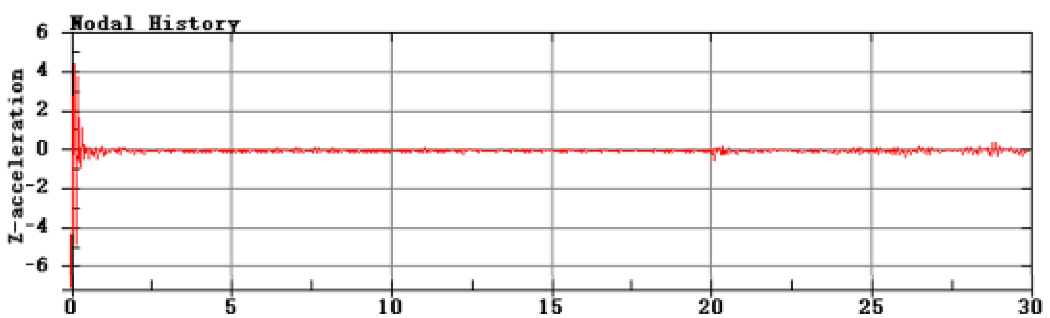
In this work, the dynamic response of submarines navigating in floating ice field was conducted based on the FEM-ALE coupled method. Different from traditional icebreakers, the submarine almost only collides with the first ice floe, and the remaining floes are pushed aside without accumulating. The collision is a continuous loading–unloading process, and its frequency is negatively correlated with the three working condition factors. The intensity of dynamic response of the submarine is generally positively correlated with the three working condition factors, but it is locally influenced by the relative position of the collision. All three working condition factors affect the degree of ice floe flipping, thereby influencing the relative collision position.

In this work, plastic deformation of the structure only occurred under the conditions of an ice thickness of 1.2 m, floating ice size of 6 m by 6 m, and navigation speeds of 6 knots and 4 knots. Therefore, it is recommended that the structure should try to avoid more severe conditions than an ice thickness of 1.2 m, a floating ice size of 6 m by 6 m, and a navigation speed of 4 knots when navigating on floating ice field. Based on the simulation results in this paper, an updated ice resistance method was developed by introducing the floating ice size to the Colbourne method, which was validated using a 5 m × 5 m condition.

Due to the extensive computational time required for each scenario in this study, the mechanism of the impact of floating ice flipping on collisions was not quantitatively investigated. The critical working conditions currently proposed are estimated values that require further refinement into more accurate values through additional research. The empirical equation improvement scheme presented in this paper, based on simulation results, needs to be validated through model tests.

References

1. Huang, L.; Li, Z.; Ryan, C.; Ringsberg, J.W.; Pena, B.; Li, M.; Ding, L.; Thomas, G. Ship resistance when operating in floating ice floes: Derivation, validation, and application of an empirical equation. Mar. Struct 2021, 79, 103057. [Google Scholar] [CrossRef]
2. Ghosh, S.; Rubly, C. The emergence of Arctic shipping: Issues, threats, costs, and risk-mitigating strategies of the Polar Code. Aust. J. Marit. Ocean Aff. 2015, 7, 171–182. [Google Scholar] [CrossRef]
3. Xue, Y.; Liu, R.; Li, Z.; Han, D. A review for numerical simulation methods of ship-ice interaction. Ocean Eng. 2020, 215, 107853. [Google Scholar] [CrossRef]
4. Li, F.; Huang, L. A review of computational simulation methods for a ship advancing in broken ice. J. Mar. Sci. Eng. 2022, 10, 165. [Google Scholar] [CrossRef]
5. Huang, L.; Li, M.; Igrec, B.; Cardiff, P.; Stagonas, D.; Thomas, G. Simulation of a ship advancing in floating ice floes. In Proceedings of the Port and Ocean Engineering under Arctic Conditions (POAC), Delft, The Netherlands, 9–13 June 2019. [Google Scholar]
6. Runeberg, R. On steamers for winter navigation and ice-breaking (including plates at back of volume) Minutes of the Proceedings. Thomas Telford 1889, 97, 277–301. [Google Scholar]
7. Shimansky, J.A. Conditional standards of ice qualities of a ship. ISA Trans. 1938, 130, 1–381. [Google Scholar]
8. Kashteljan, V.I.; Poznjak, I.I.; Ryvlin, A.J. Ice Resistance to Motion of a Ship; Sudostroenie: Leningrad, Russia, 1969. [Google Scholar]
9. Jones, S.J. Ships in ice-a review. In Proceedings of the 25th Symposium on Naval Hydrodynamics, Washington DC, USA, 8–13 August 2004; National Academies Press: Washington, DC, USA, 2004; Volume 3, pp. 78–85. [Google Scholar]
10. Lindqvist, G. A straightforward method for calculation of ice resistance of ships. In Proceedings of the POAC, Luleå, Sweden, 12–16 June 1989; pp. 722–735. [Google Scholar]
11. Riska, K. Performance of Merchant Vessels in Ice in the Baltic; Sjafartsverket: Norrköping, Sweden, 1997. [Google Scholar]
12. Bronnikov, A.V. Analysis of resistance of cargo ships going through pack ice. Trans. Leningr. Shipbuild. Inst. 1959, 24, 13. [Google Scholar]
13. Mellor, M. Ship resistance in thick brash ice. Cold Reg. Sci. Technol. 1980, 3, 305–321. [Google Scholar] [CrossRef]
14. Daley, C.G. Ice Edge contact-A brittle failure process model. Loads 1991, 144, 1–92. [Google Scholar]
15. Cho, S.R.; Jeong, S.Y.; Lee, S. Development of effective model test in pack ice conditions of square-type ice model basin. Ocean Eng. 2013, 67, 35–44. [Google Scholar] [CrossRef]
16. Kim, M.C.; Lee, W.J.; Shin, Y.J. Comparative study on the resistance performance of an icebreaking cargo vessel according to the variation of waterline angles in pack ice conditions. Int. J. Nav. Archit. Ocean Eng. 2014, 6, 876–893. [Google Scholar] [CrossRef] [Green Version]
17. Jeong, S.Y.; Choi, K. A review on ice resistance prediction equation for icebreaking vessels. In Proceedings of the 19th International Offshore and Polar Engineering, Conference, Chennai, India, 20–24 September 2009; pp. 587–592. [Google Scholar]
18. Wang, C.; Sun, W. A review of the resistance forecast method of icebreaker. Ship Sci. Technol. 2015, 37, 1–8. [Google Scholar]
19. Xiang, J.; Munjiza, A.; Latham, J.P.; Guises, R. On the validation of DEM and FEM-DEM models in 2D and 3D. Eng. Comput. 2009, 26, 673–687. [Google Scholar] [CrossRef]
20. Huang, L.; Tuhkuri, J.; Igrec, B.; Li, M.; Stagonas, D.; Toffoli, A.; Cardiff, P.; Thomas, G. Ship resistance when operating in floating ice floes: A combined CFD&DEM approach. Mar. Struct. 2020, 74, 102817. [Google Scholar]
21. Zhang, M.; Garme, K.; Burman, M.; Zhou, L. A Numerical Ice Load Prediction Model Based on Ice-Hull Collision Mechanism. Appl. Sci. 2020, 10, 692. [Google Scholar] [CrossRef] [Green Version]
22. Tsarau, A.; Lubbad, R.; Løset, S. A numerical model for simulation of the hydrodynamic interactions between a marine floater and broken sea ice. Cold Reg. Sci. Technol. 2014, 103, 1–14. [Google Scholar] [CrossRef]
23. Ji, H.; Zhang, J. Fluid-structure interaction method for ice-column collision based on cohesive element method. Shock Vib. 2023, 42, 41–47+74. [Google Scholar]
24. Song, M.; Kim, E.; Amdahl, J.; Greco, M.; Souli, M. Numerical Investigation of Fluid-Ice-Structure Interaction During Collision by an Arbitrary Lagrangian Eulerian Method. In Proceedings of the International Conference on Ocean, Offshore and Arctic Engineering Omae, Busan, Republic of Korea, 18–24 June 2016. [Google Scholar]
25. Su, B.; Riska, K.; Moan, T. Numerical study of ice-induced loads on ship hulls. Mar. Struct. 2011, 24, 132–152. [Google Scholar] [CrossRef]
26. Chai, W.; Leira, B.J.; Naess, A. Short-term extreme ice loads prediction and fatigue damage evaluation for an icebreaker. Ships Offshore Struct. 2018, 13 (Suppl. S1), 127–137. [Google Scholar] [CrossRef]
27. Zhao, W.; Leira, B.J.; Kim, E.; Feng, G.; Sinsabvarodom, C. A probabilistic framework for the fatigue damage assessment of ships navigating through level Ice fields. Appl. Ocean Res. 2021, 111, 102624. [Google Scholar] [CrossRef]
28. Zhao, W.; Leira, B.J.; Feng, G.; Gao, C.; Cui, T. A reliability approach to fatigue crack propagation analysis of ship structures in polar regions. Mar. Struct. 2021, 80, 103075. [Google Scholar] [CrossRef]
29. Zheng, Y. Research on Calculation Method of Ice Load for Polar Heavy Icebreaker. Ph.D. Thesis, Harbin Engineering University, Harbin, China, 2019. [Google Scholar]
30. Gao, Y. An Elastic-Plastic Ice Material Model and Iceberg Shape Sensitivity Analysis for Ship-Iceberg Collision Scenario. Ph.D. Thesis, Shanghai Jiao Tong University, Shanghai, China, 2015. [Google Scholar]
31. Lu, S.; Shen, H.T. Constitutive laws for river ice dynamics. Ice Surf. Wate 1998, 32, 109–116. [Google Scholar]
32. Mao, F. Study on the Bow Configuration of Polar Sailing Ship Based on Icebreaking Capacity. Master’s Thesis, Harbin Engineering University, Harbin, China, 2017. [Google Scholar]
33. Zhang, X. Numerical Simulation of Fluid-Structure Interaction Arising from Bottom Slamming. Master’s Thesis, Dalian University of Technology, Dalian, China, 2007. [Google Scholar]
34. Ni, B.Y.; Huang, Q.; Chen, W.S. Numerical simulation of ice resistance of ship turning in level ice zone considering fluid effects. J. Ship Res. 2020, 15, 1–7. [Google Scholar]
35. Colbourne, D.B. Scaling pack ice and iceberg loads on moored ship shapes. Ocean. Eng. Int. 2000, 4, 39–45. [Google Scholar]
Figure 1. Simplified schematic diagram of elastic-plastic model [31].
Jmse 11 01560 g001
Figure 2. Schematic diagram of mesh movement.
Jmse 11 01560 g002
Figure 3. The numerical model for structure-ice interaction.
Jmse 11 01560 g003
Figure 4. (a) The distribution of pressure gradient; (b) the pressure at monitored nodes.
Jmse 11 01560 g004
Figure 5. The time history of the ice floe’s acceleration.
Jmse 11 01560 g005
Figure 6. (a) The relation between lnFrp and lnCp; (b) the comparison of ice resistance between theory and numerical simulation.
Jmse 11 01560 g006
Figure 7. (a) loading stage; (b) unloading stage.
Jmse 11 01560 g007
Figure 8. (a) The structure-ice interaction at 6 kn; (b) the structure-ice interaction at 4 kn; (c) the structure-ice interaction at 2 kn; (d) the structure-ice interaction at 1 kn.
Jmse 11 01560 g008
Figure 9. The ice resistance at different navigation speeds.
Jmse 11 01560 g009
Figure 10. (a) The effective stress at 6 kn; (b) the structural deformation at 6 kn; (c) the effective stress at 4 kn; and (d) the structural deformation at 4 kn.
Jmse 11 01560 g010
Figure 11. (a) The structure-ice interaction with size 2 m × 2 m of the ice floe; (b) the structure-ice interaction with size 4 m × 4 m of the ice floe; (c) the structure-ice interaction with size 6 m × 6 m of the ice floe.
Jmse 11 01560 g011
Figure 12. The ice resistance with different ice floe size.
Jmse 11 01560 g012
Figure 13. (a) The effective stress at 6 m × 6 m; (b) the structural deformation at 6 m × 6 m.
Jmse 11 01560 g013
Figure 14. (a) The result animation of 0.5 m working condition t = 1.15 s; (b) the resulting animation of 0.5 m working condition t = 4.40 s.
Jmse 11 01560 g014
Figure 15. The ice resistance at different ice thickness.
Jmse 11 01560 g015
Figure 16. The structural response at different ice thicknesses.
Jmse 11 01560 g016
Figure 17. The relation between lnFrp and lnCp.
Jmse 11 01560 g017