Article

The State of the Hydrographic Survey and Assessment of the Potentially Risky Region for Navigation Safety

1
Faculty of Maritime Studies, University of Split, Ruđera Boškovića 37, 21000 Split, Croatia
2
Plovput d.o.o., Obala Lazareta 1, 21000 Split, Croatia
*
Author to whom correspondence should be addressed.
J. Mar. Sci. Eng. 2023, 11(8), 1498; https://doi.org/10.3390/jmse11081498
Submission received: 5 June 2023 / Revised: 17 July 2023 / Accepted: 23 July 2023 / Published: 27 July 2023
(This article belongs to the Special Issue Recent Research on Sustainable and Safe Maritime Transportation)

Abstract

:
The hydrographic survey is an important technology for improving maritime safety, especially in coastal waters. The accuracy of nautical charts and navigation publications is known to be directly related to hydrographic survey data. Therefore, this paper aims to investigate the status of a hydrographic survey by the International Hydrographic Organization (IHO) regions and identify the potentially risky IHO region for navigation safety. The fundamental step was to obtain the qualitative and quantitative data of the survey. Then, the presented analysis includes investigating the possible relationships between survey status and geographical characteristics by IHO regions. Considering that coastline length and sea surface data have not been calculated by regions, a quantum geographic information system was used to extract data. Using the presented methodology, the case study analyzes the data of stranded ships from 2010 to 2021 by IHO regions, estimates coastline length and sea surface by regions, and establishes the relationships between the coastline length, sea surface, and stranded ships. The results point out the need for improvement in the state of the hydrographic survey in almost all IHO regions and show a correlation between the sea surface and an adequate survey, as well as the coastline length and stranded ships. Hence, this research indicates the possibility of rationalizing the distribution of the IHO region concerning the sea surface and coastline length.

1. Introduction

A hydrographic survey is a procedure for surveying marine waters and underwater topography to ensure the safety of navigation [1]. It is carried out according to the standards and specifications defined by the International Hydrographic Organization (IHO) [2,3]. The IHO divided the world into 15 regions and encouraged the establishment of Regional Hydrographic Commissions (RHCs) to coordinate hydrographic activity and cooperation at the regional level [4]. The RHCs are made up of IHO member states, together with other regional states that wish to participate. Therefore, the task of the RHCs task is to complement the work of the IHO at the regional level. It is well-known that the importance of hydrographic surveys is related to obtaining accurate data. Also, it is to make nautical charts and navigation publications with particular emphasis on the possibilities that may affect the safety of navigation [5,6]. Navigation charts are essential tools for marine navigation, especially when it is known that more than 80% of international world trade occurs at sea [7,8].
Despite all the efforts of the IHO to improve the state of implementation of hydrographic surveys in the world, the problem of accuracy and coverage of the survey still exists. In the last few decades, the need for adequate coverage of hydrographic surveys and the production of nautical charts and navigation publications has increased [9]. Some of the critical factors that influenced this were the increasing number of very large crude carriers with extremely large drafts, the need to protect the marine environment, changes in maritime trade patterns, the increasing importance of seabed resources, etc.
A large percentage of the world’s seas, straits, and ports do not have adequate nautical chart coverage. Many nautical charts that were accurate and reliable in previous years do not represent today’s real situation. Most charts contain a mixture of surveys of differing quality or rely on data from hydrographic survey methods that were limited. Although current technical and technological solutions for implementing a hydrographic survey demonstrate high development, they are incomplete and inaccurate [3,10,11,12].
A lack of relevant hydrographic survey information can lead to maritime accidents and hinder maritime trade development [13]. Maritime causalities often result from several factors, and it is very difficult to conclude whether this situation is caused solely by inadequate hydrographic data. It can be concluded that incomplete and inaccurate hydrographic data are one of the causes of maritime accidents that can result in shipwrecks.
In the present study, the main contribution is to identify the potential risk regions for navigation and point out the possibility of rationalizing the distribution of the IHO region concerning the sea surface and coastline length. Therefore, the aim of this study is to investigate the quantitative and quality status of hydrographic surveys in IHO regions, to analyze the data of stranded ships from 2010 to 2021 by IHO regions, to estimate coastline length and sea surface by regions, and to establish relationships between the coastline length, sea surface, and stranded ships.
The rest of the paper is arranged in the following manner. Section 2 presents a literature review. Section 3 describes and discusses the methodology utilized in this study. The case study results are presented and discussed in Section 4. Section 5 presents the limitations of the study. Finally, Section 6 concludes the study and provides recommendations for future studies.

2. Literature Review

Based on previous research, the authors’ points of interest can generally be divided into traditional and modern or remote hydrographic survey techniques. The importance of accurate bathymetric and hydrographic data is recognized. The authors of [14,15,16,17,18,19] proposed and analyzed methods and algorithms that will make it easier to recognize the data obtained by using multi-beam echosounder datasets. Onwards, new correction methods were researched and proposed to obtain data using air and satellite platforms [20,21,22,23,24,25]. Additionally, the impact of new technologies and computational techniques, such as deep learning and artificial intelligence, is investigated [26,27,28,29,30,31,32,33].
Within the hydrographic and bathymetric survey field, some studies were based on the methodology of survey planning [10,34,35,36]. They emphasized the importance of defining priorities that would ultimately reduce risks and increase hydrographic surveying [35,36]. The problem with some areas, such as the Arctic, Antarctic, and some tropical areas, is due to the fact that they are under pressure to increase vessel transits, as well as tourism and exploration of natural resources, as recognized in [37]. They are relatively unknown in terms of hydrographic surveys and nautical chart content.
The importance of safe maritime transport, quantifying the risk level of the operating world fleet, and developing a risk management process has become the focus of some authors. Statistical analysis regarding the main causes for major types of collision, contact, stranding, fire, explosion, and failure of machinery equipment is presented in [38]. A chronological overview of the contribution of ship stranding frequency is presented in [39]. The stranding, causes, and risk assessments are investigated and discussed in [40,41]. The authors of [42,43,44] presented a statistical analysis of ship accidents and the relationship between accident rates and ship age. Onwards, risk estimation based on accident analysis is performed by [45,46]. Most of the literature investigates the main factors influencing maritime accidents, including labor conditions, seafarer competence, situation awareness, and so on [47,48,49,50,51]. Extensive and detailed research on the risk indicators in maritime accidents and how they are considered in reporting maritime accidents are presented in [52].
To improve maritime safety, the state of hydrographic surveying, and nautical chart accuracy, the IHO divided the world into regions. It has to be pointed out that, from the available literature, the geographical disparity between IHO regions has not been explored so far. Some authors recognized the importance of the coastline for various applications, such as coastal zone management, navigation safety, etc. [53,54,55,56]. Geographical information system (GIS) technology is used to extract coastlines and analyze the changes. A dedicated geographic information system (GIS) for satellite-based bathymetry estimation is represented in [57].
Based on the available literature and from everything presented, it is reasonable to investigate the proposed research and aims.

3. Methodology

Considering the aim of the study and that the riskiness of a particular region for navigation is closely related to the state of the hydrographic survey, we propose the methodological framework as shown in Figure 1. Also, the potential problem of the survey state in some regions can be influenced by the dimensions of important geographical characteristics, for instance, coastline length and sea surface.
Figure 1 shows that the presented methodology consists of five stages, which are explained in detail in the next sections.

3.1. Stage 1: Analysis of the Current State of the Hydrographic Survey by IHO Regions

This stage consists of obtaining information on the current status of the hydrographic survey. The main source of hydrographic survey data is the IHO Publication C-55 [58]. The publication’s content is maintained in a database on the IHO website and includes data for 90% of the world’s coastal states. It should be noted that each member state entered the data into its designated area. Furthermore, to obtain the status of the hydrographic survey by the IHO regions, the following procedure is proposed, as shown in Figure 2.
As shown in Figure 2, the represented procedure consists of three steps. The first step, data collection, includes loading the data from IHO Publication C-55 into the database. The second step, data analysis, is divided into three parts: grouping of data by the IHO region, grouping of data by the state of the hydrographic survey, and calculating the arithmetic mean from the data, considering every IHO region, using Equation (1) [59]:
x ¯ = x 1 + x 2 + + x i N = 1 N i = 1 n x i
where x i is the single value of the variable and N is the total number of data.
Finally, the third step is reserved for the results and interpretation. The final step includes data visualization and knowledge extraction.

3.2. Stage 2: Determining Coastline Length and Sea Surface by IHO Regions

The coastline length and sea surface are among the country’s most important geographical characteristics [60]. To the best of our knowledge, these mentioned characteristics have never been calculated for the IHO regions. These calculations were performed in this study using the quantum geographic information system QGIS software. QGIS is an open-source geographic information system licensed under the GNU general public license. QGIS allows the capture, storage, query, analysis, and display of geospatial data [61,62]. The general framework for QGIS is shown in Figure 3.
QGIS has a built-in function and algorithms to calculate various properties based on the feature’s geometry, such as line length and area. The coastline length and sea surface of each IHO region were calculated via automation, which was designed in a QGIS environment with an integrated approach involving several procedures. The methodology details are represented in the process flowchart in Figure 4.
IHO regional boundaries were extracted from existing data from the “IHO web catalogue” [63] and georeferenced with data from “IHO world seas” data [64]. Georeferencing requires using QGIS software to assign new coordinates according to the shapefile by applying a geometric transformation. The affine transformation function is used and can be represented as expression (2) [65]:
x = A x + B y + C y = D x + E y + F
where x and y are the coordinates of the input layer; x and y are the transformed coordinates; A ,   B ,   C ,   D ,   E ,   a n d   F are determined by comparing the locations of the source and destination control points.
The IHO coastline was extracted from the “IHO world seas” data. Since polygons represent the seas, it was necessary to convert them into lines to get the shape line of the world’s coastline. The boundaries of the IHO regions and IHO coastlines were made and extracted in the new shapefiles to the reference input data. The new shapefiles are created for each feature: the points, polylines, and polygons, and they need to be georeferenced to the reference data.
The coastline length of each IHO region was obtained using a vector geometry tool to reference the input data. Every point P x , y in R 2 can be represented by its point vector, as shown in expression (3) [66,67]:
P = x y
The length of a vector in R 2 is defined using (4):
P = x 2 + y 2
Polylines within the boundaries of IHO regions that correspond to the region’s coastline have been calculated for length using the QGIS vector geometry tool. From the gained boundaries, polygons of the IHO regions were made. The surfaces of these polygons that correspond to the sea surface of a given region were calculated using vector geometry algorithms embedded in QGIS tools.

3.3. Stage 3: Calculating the Correlation between Hydrographic Survey Status and Geographical Characteristics between IHO Regions

Various techniques can be used to analyze the correlation relationships in the dataset. Furthermore, the Pearson correlation has been adopted to identify the impact of coastline length and sea surface on the status and quality of the hydrographic survey. This is a statistical analysis of the colinear relationships between variables and represents the most common method for numerical variables [68]. Pearson’s correlation coefficient, considering two variables, can be calculated using Equation (5) [69]:
C A , B = C o v a r i a n c e ( A , B ) σ A σ B
where C A , B is the correlation coefficient,  C o v a r i a n c e ( A , B ) is the covariance, and σ A and σ B are the standard deviations of variables A and B.
The correlation coefficient for a dataset of two sets, a 1 , a 2 , , a n and b 1 , b 2 , , b n , can be calculated using Equation (6) [69,70]:
C = i = 1 n ( a i a ¯ ) ( b i b ¯ ) i = 1 n ( a i a ¯ ) 2 i = 1 n ( b i b ¯ ) 2
where n is the sample size, a i and b i are the ith data values, and a ¯ , b ¯ are the mean values.
It is well known that the Pearson correlation coefficient value changes between −1 and 1 [71,72,73]. The value of the correlation coefficient from 0 to 1 is positive, indicating the proportional growth of values in both datasets. A correlation coefficient value from 0 to −1 indicates a negative correlation, i.e., a rise in the value of one variable that is proportional to a decline in the value of the other. The strength of the association for different ranges of the coefficient is shown in Table 1 [73].

3.4. Stage 4: Analysis of Stranded Ships by IHO Regions

Under the Safety of Life at Sea (SOLAS) regulation and marine pollution (MARPOL) international convention, the IMO requires respective nation-states to submit accident casualty reports to their global integrated shipping information system (GISIS) [52]. In this stage, publicly available stranded ship reports submitted to the IMO from 2010 to 2021 were used as the data source. The obtained data are classified according to the IHO regions with regard to the known position of the stranding, which has never been performed before.
In order to examine the relationships between coastline length and sea surface with respect to the number of stranded ships by the IHO regions, the correlation is calculated.

3.5. Stage 5: Results and Conclusions

This stage is the final part of the proposed methodology. In addition, the results are obtained and analyzed. The conclusions are presented and explained.

4. Results and Discussion

The case study of this paper is composed of two main parts. The first part includes the hydrographic survey results, coastline length, and sea surface of the IHO regions. The second relates to the data of stranded ships from 2010 to 2021 by the IHO regions and establishes relationships between the coastline length, sea surface, and stranded ships.

4.1. The Results of the Hydrographic Survey, Coastline Length, and Sea Surface by IHO Regions

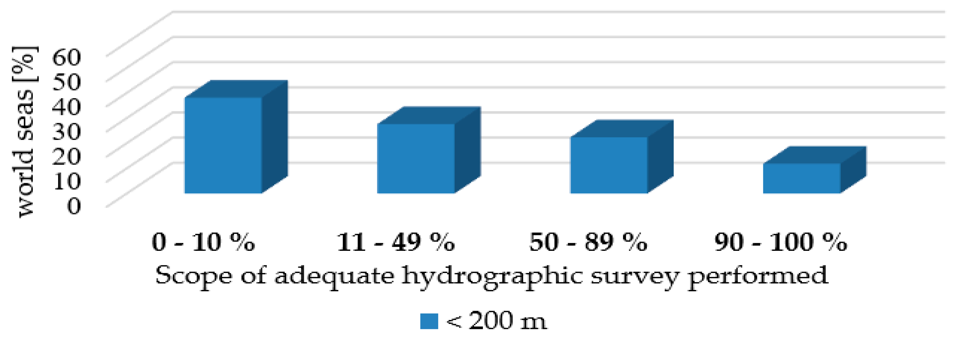
The first study stage involved obtaining information on the current status of the hydrographic survey for depths up to 200 m. This paper did not investigate the depths over 200 m because it is justifiably considered that their influence on the safety of navigation is far less significant. Each member state entered the data in its designated area, which includes the percentages of adequate, resurvey, and unsurveyed coverage. The status of implementing an adequate hydrographic survey at depths up to 200 m in world seas is calculated and shown in Figure 5.
All adequate hydrographic surveys were divided into four categories for better visibility to easier meet the goals of this study. For all of these four categories, we calculated the percentage of the total number of seas listed in [57] that performed an adequate hydrographic survey. The obtained data indicate just about 10% of the total seas performed an adequate hydrographic survey within the scope of 90–100%. Less than 20% of the seas have an adequate hydrographic survey in the scope of more than 50%. About 30% of the total number has conducted an adequate survey in the 11–49% range. Finally, almost 40% of the seas have more than 90% of their territory unsurveyed. The results of the scope of implementation of an adequate hydrographic survey worldwide point to the fact that the state of the survey is generally unsatisfactory.
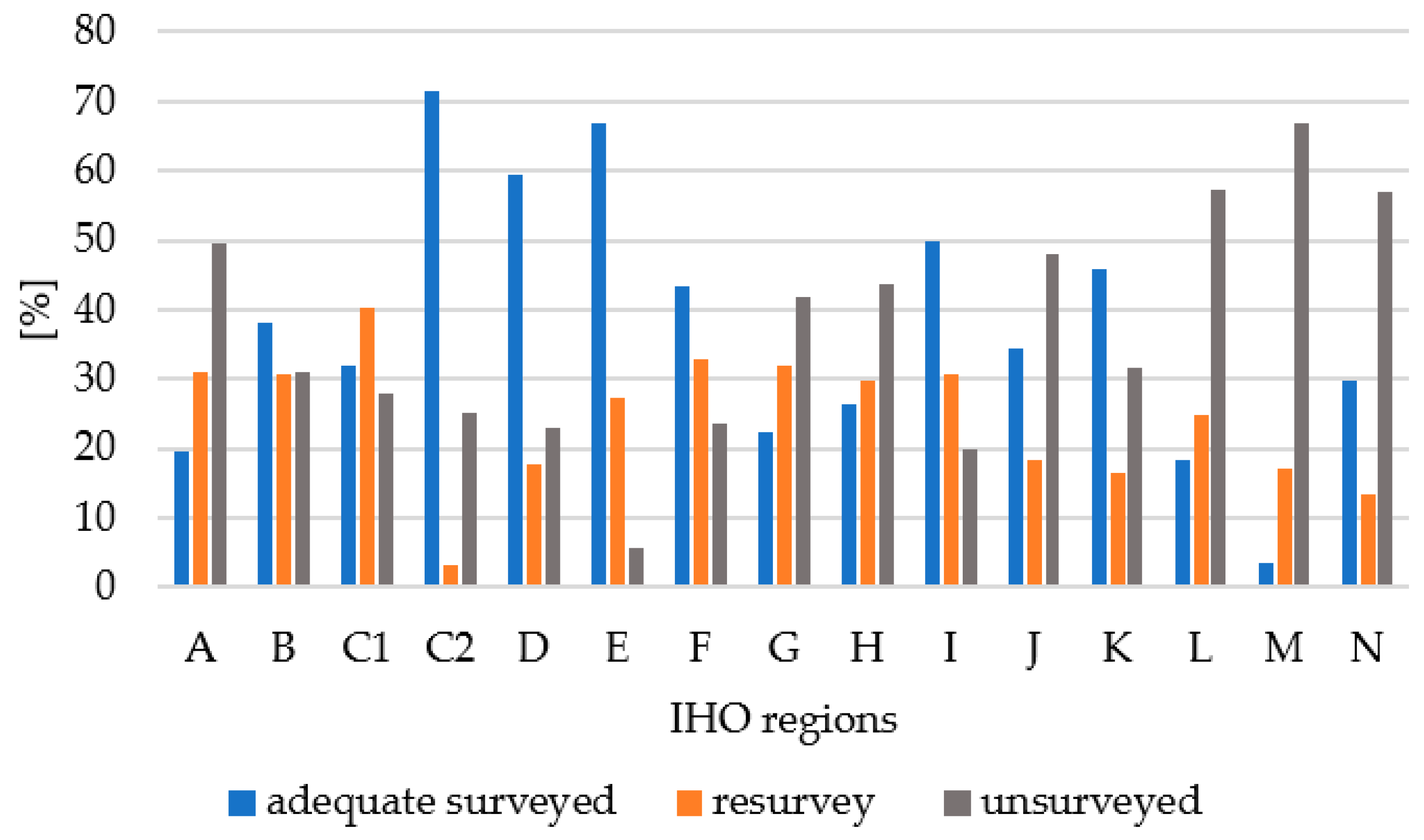
Given that the International Hydrographic Organization divides the world into 15 regions (letters from A to N), to obtain a more precise insight into the coverage of hydrographic surveys worldwide, the data regarding the IHO regions have been obtained and extracted, Figure 6.
According to Figure 6, the status of the hydrographic survey is divided into three categories: an adequate survey area (blue color), an area that needs to be resurveyed (orange color), and an area that has never been surveyed (grey color). An adequate hydrographic survey exceeding 50% of the total water is evident only in regions C2 (Southeast Pacific), D (North Sea), and E (Baltic Sea). The regions A (US/Canada), L (Southwest Pacific), and M have less than 20% of adequately surveyed sea areas. The region where it is necessary to repeat the hydrographic survey, in more than 40% of the total water, is the hydrographic region C1 (Southwest Atlantic). These regions require a resurvey due to outdated data, or the technology is not compliant with IHO standards. In regions A, G (East Atlantic), H (South Africa and Islands), J (North Indian Ocean), L, M, and N, more than 40% of the water surface at depths of up to 200 m has not been surveyed. By observing the ratio of the unsurveyed area, it can be concluded that the worst situation is in region L, except in the pole regions (regions M and N).
It is important to note that the areas that have never been surveyed and those that require a resurvey have unreliable data. Such data directly affect the reliability of nautical charts and navigation publications. Therefore, these IHO regions are potentially dangerous because they can threaten navigation safety.
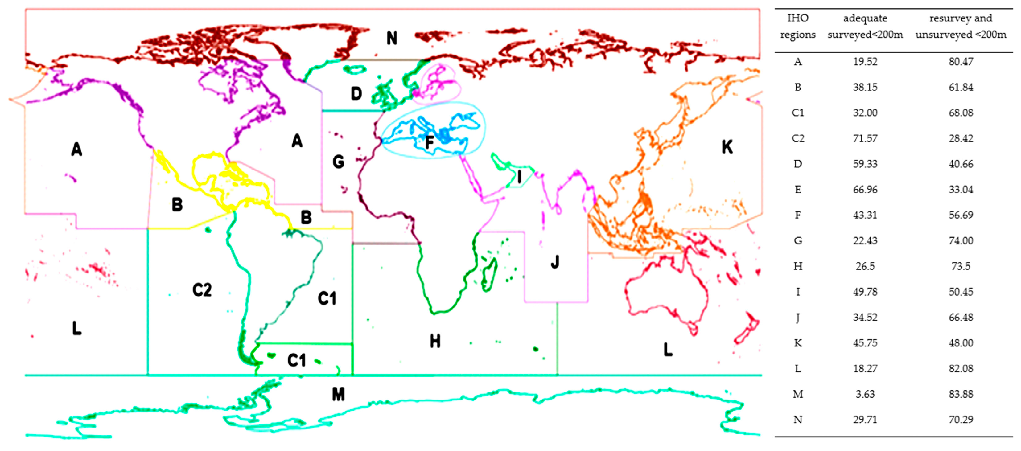
After the analysis of the current state of the hydrographic survey by IHO regions, we investigated the important geographical characteristics of the regions. Since previous research paid no attention to calculating the coastline length and the sea surface by regions, such analysis has become a subject of interest in this paper. The final appearance of the IHO regions made in QGIS, which can be further manipulated to calculate geographical parameters, is shown in Figure 7.
Based on the model in Figure 7, the coastline length and sea surface calculations for the IHO regions have been performed using QGIS algorithms. It is possible to notice the ratio of reliable and unreliable sea areas. The IHO regions with more than 50% of total water not adequately surveyed are A, B (Middle America and Caribbean), C1 (Southwest Atlantic), F (The Mediterranean and the Black Sea), G, H, I (Persian Gulf), J, L, M, and N regions. The mentioned regions represent more than 70% of the total IHO regions. Using this approach, it is possible to assume potentially risky regions. The most challenging situation is in the hydrographic regions A, G, H, L, M, and N, where more than 70% of the total water needs to be adequately surveyed.
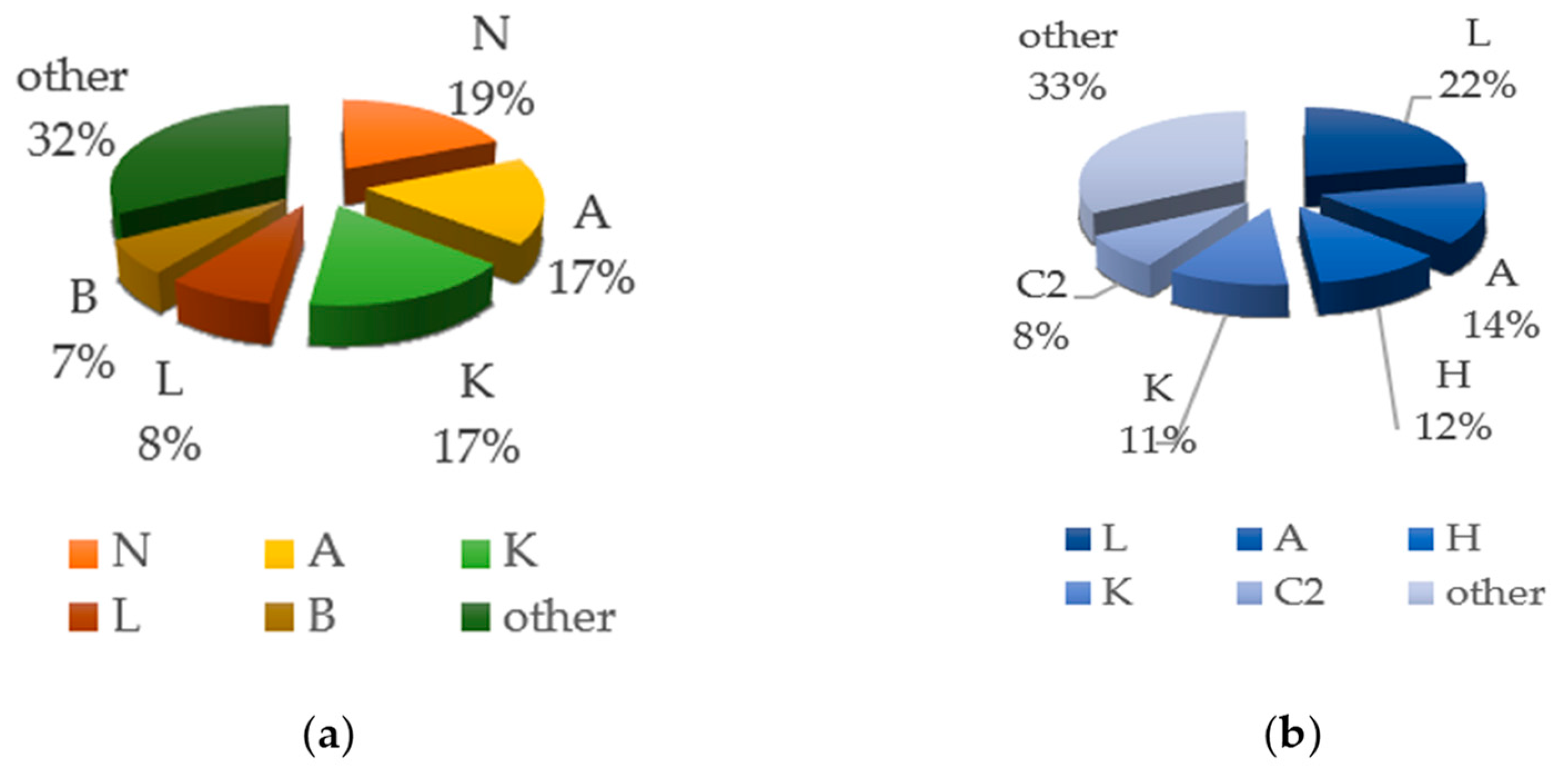
The data relating to the highest values of individual characteristics depending on the IHO regions are presented in Figure 8.
According to Figure 8a, it can be noticed that more than 60% of the world’s sea coastline belongs to four regions, N, A, K, and L. In terms of the sea surface area (Figure 8b), almost 60% belongs to four regions, L, A, H, and K, out of which region L encompasses 22% of the total surface area.
The presented analysis also includes a deeper investigation of a possible relationship between the coastline length, sea surface, and the status of a hydrographic survey by IHO regions. The strength of the relationship between the two variables is determined by performing a Pearson correlation analysis. The six attributes tested for correlation, Table 2, and their graphical reviews are presented in Figure 9.
Table 2 shows the selected attributes, including geographical characteristics by the IHO regions and attributes that determine the status of a hydrographic survey by regions. Geographical characteristic attributes refer to the sea surface and coastline length. The other attributes include adequate survey, need to be resurveyed, unsurveyed, and inaccurate data.
A higher number of coefficients indicates that the two variables have a strong correlation, and a lower value indicates otherwise [69]. Each factor correlates 1 with itself, resulting in a total of 21 possible relationships between factors. Based on Table 2, and regarding the rules from Table 1, the inaccurate data and unsurveyed were strongly positively correlated (C = 0.845). Furthermore, there are two strongly negative correlations: one is between the adequate survey and the unsurveyed (C = −0.865), and the other is between the adequate survey and inaccurate data (C = −0.983). There is a moderately negative association between the sea surface and an adequate survey (C = −0.516). Also, a moderate positive association exists between the sea surface and the unsurveyed (C = 0.631). The correlation between attribute points and coastline length has no significant effect on the status of the hydrographic survey by the IHO regions. The obtained correlation coefficients show that variables with adequate survey, inaccurate data, and unsurveyed variables have very strong relationships. Contrarily, the variable coastline length has weak or non-existent correlations with all other variables, which indicates that the variable is an appropriate choice to investigate the other variables. The sea surface variable has weak to moderate correlations with the other variables and an almost non-existent correlation with the coastline surface variable (C = 0.146). Due to weak or moderate dependence relationships with other variables, variables such as sea surface and coastline length with the stranded ships variable are chosen as variables to identify the potential risk region for navigation and point out the possibility of rationalizing the distribution of the IHO region concerning the sea surface and coastline length.

4.2. Stranded Ships from 2010–2021 by IHO Regions (Case Study Results)

This section presents the proposed methodology using 15 IHO regions with coastlines and sea surfaces. We show the relationships between the coastline length, sea surface, and stranded ships. Table 3 shows the variables from all 15 IHO regions.
In Table 3, three variables are presented for all 15 IHO regions (A–N). The first variable, the sea surface, represents the estimated sea surface area for each IHO region. It is calculated using the methodology described in Section 3.2 and represents the contribution of the proposed paper. The second variable, the coastline length, represents the length that bounds the sea surface for each IHO region. Also, it represents the proposed paper’s contribution and is estimated using the methodology described in Section 3.2. It should be noted that these two variables represent the geographical characteristics of the IHO regions. They are chosen because both variables have non-existent or weak correlations with other variables (Table 2). Finally, the third variable, the stranded ships, represents the number of stranded ships in each IHO region. They were collected between 2010 and 2021. Also, the total number of stranded ships (denoted as Total) is also included in the study as a variable. From the table, it can be observed that the total number of stranded ships from 2010 to 2021 is 593. Further, the number of stranded ships has declined over the years. Also, regions F and K, which cover the Mediterranean and Pacific regions, respectively, had the most stranded ships in the last 12 years: 122 and 111, respectively. Regions M and N, which cover the Artic and Antarctica regions, respectively, had the least number of stranded ships in the last 12 years: 1 and 7. The sea surface variables and coastline length are shown in Figure 8, which shows the percentage coverage for each IHO region.
It can be observed that regions F and K occupy 0.08% and 1.09% of the world’s sea surface, and 3.15% and 16.73% of the coastline length, respectively. Similarly, regions M and N occupy 57.90% and 33.60% of the world’s sea surface, and 2.76% and 18.90% of the coastline length, respectively.
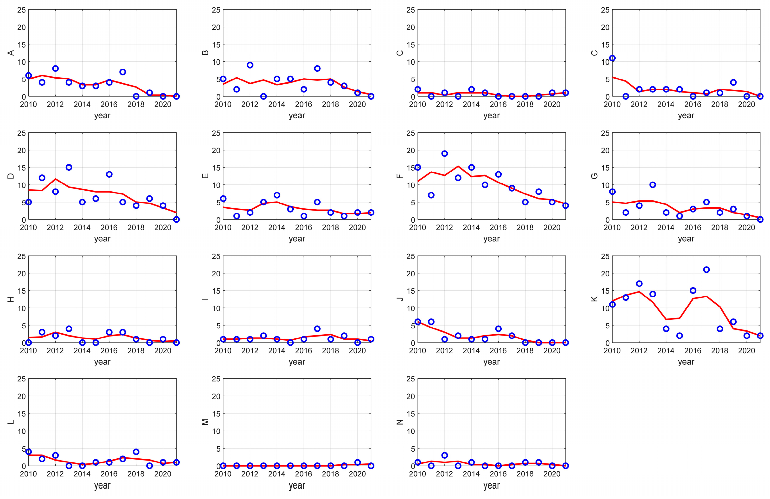
To establish a relationship between coast length, sea surface, and maritime causalities concerning IHO regions and to prove the proposed concept, data obtained from a number of stranded ships are processed in the following procedure. Moving average filtering, with k = 3, is performed to eliminate outliers in the number of stranded ships from 2010 to 2021. Such a procedure is shown in Figure 9.
A weighting method is performed since each IHO region occupies a different sea surface and has a different coastline length, i.e., when performing the correlation analysis, it is necessary to consider such variations. Weights are obtained by transforming the percentage of variables sea surface and coastline length in decimal numbers and multiplying with the variable number of stranded ships, respectively. This provides a weighted number of stranded ships per coastline length and a weighted number of stranded ships per sea surface.
A Smirnov–Kormogolov test was performed on the sea surface, the coastline length, and the number of stranded ship variables to check if the data were normally distributed. The test showed that the variables did not have a normal distribution.
Next, correlation coefficients (5) and (6) were analyzed for the following variables: the number of stranded ships, sea surface, and coastline length, and the results are shown in Table 4.
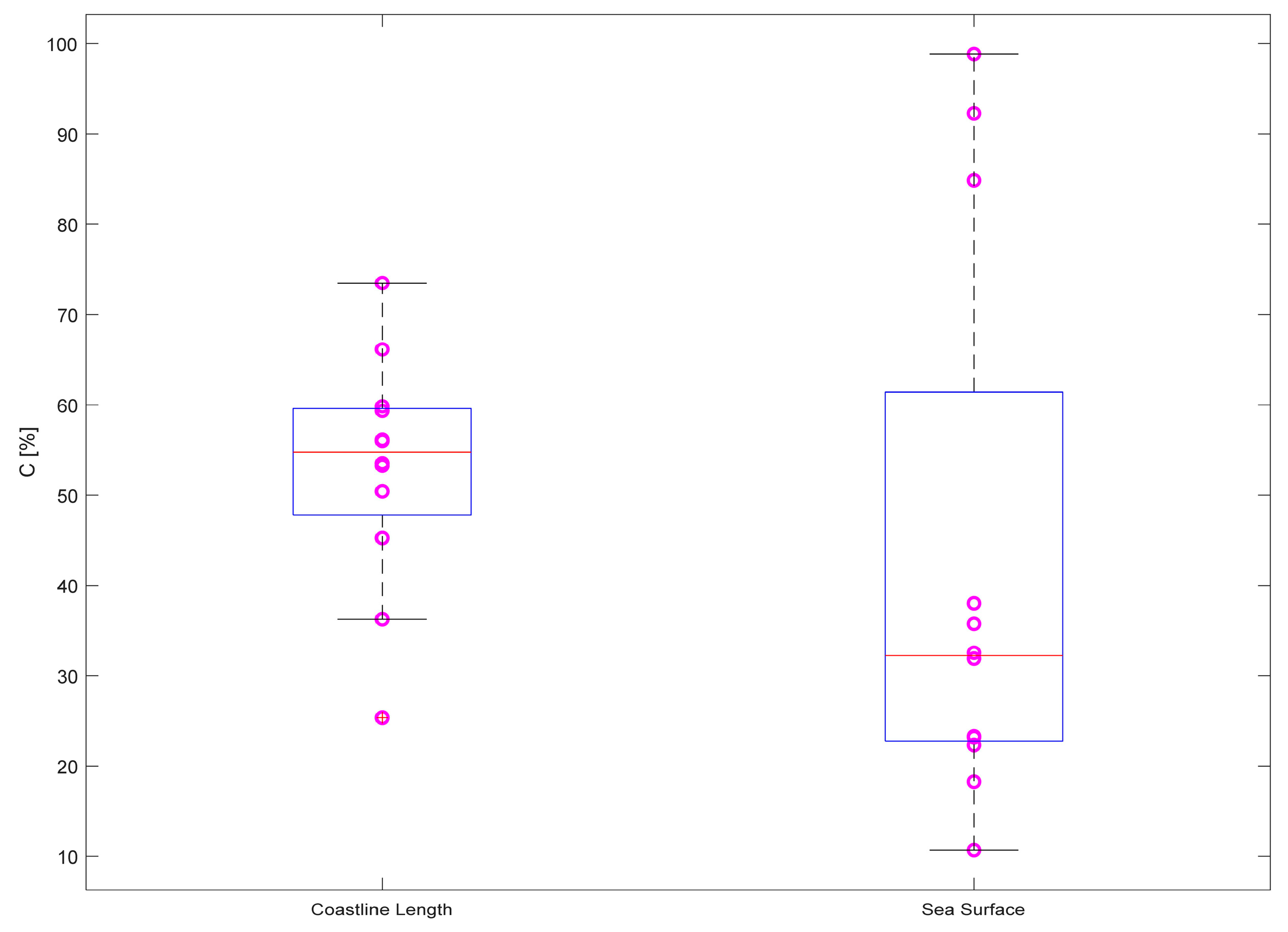
From Table 4., it can be observed that the correlation coefficients between variables, the number of stranded ships, and coastline length are between 67.44% (p < 0.01) and 32.02% (p = 0.244), with an average of 54.77%, which indicates moderate relationships. Also, correlations between the sea surface and the number of stranded ships for 12 years range between 18.24% (p = 0.515) and 98.83% (p < 0.01), with an average of 32.21%, which indicates weak relationships. Furthermore, if two correlations are compared and investigated, the results would be as shown in Figure 10.
Figure 10 shows that the coastline length variable has a higher average correlation coefficient and lower standard deviation than the sea surface variable, which shows that the number of stranded ships has a weaker dependence on the sea surface variable. If we perform a two-sided Wilcoxon rank sum test since the Smirnov–Kormogolov test rejected the null hypothesis that two samples have a normal distribution, we would obtain p = 0.078 (z = 1.7609). This shows that there is no statistical significance between the two analyses. Considering that ship strandings are related to shallow waters and coastlines, the expected results are a weak correlation between stranded ships and the sea surface.

5. Limitations of the Study

The content of IHO publication C-55, which is used as the main source of hydrographic survey data, includes 90% of the data. The most significant gaps, where data are not available for analysis, are found in Central America, the Mediterranean, the Black Sea, some parts of the Indian Ocean and neighboring seas, and the South Chines Sea and neighboring straits and seas [14]. The information provided in C-55 is not entirely accurate since it is left to each state to determine how to use the data to estimate the percentages of adequate survey coverage. Therefore, it is justifiably considered that the state of coverage by adequate measurement covers a smaller area than that shown in the study’s analysis. For the reasons mentioned above, a global picture of the implementation of hydrographic surveys by the IHO regions is provided in this paper.
The data obtained using QGIS related to the coastline length and sea surface by the IHO regions are not entirely accurate. The task of shoreline extraction and the sea surface is very difficult because the coastal area is highly dynamic and environmentally sensitive to many physical processes. The exact extraction requires knowledge of using algorithms and methods. Nevertheless, we acknowledge the importance of obtaining the baseline coastline length and sea surface data. The mentioned data are indicative of the differences between the IHO regions and the comparison analysis performed in this study.

6. Conclusions

The International Hydrographic Organization has adopted standards and recommendations for conducting hydrographic surveys to achieve the maximum standardization of nautical charts, navigation publications, services, and hydrographic surveying practices. Despite many efforts, the state of the hydrographic surveys remains unsatisfactory. The proposed research has exposed, confirmed, and represented this fact. An analysis of the hydrographic survey status in the world seas was conducted using the data acquired from the IHO publication C-55 and standard statistical metrics. Also, at depths of up to 200 m, approximately 10% of the total seas listed in the C-55 performed an adequate hydrographic survey in the 90–100% range.
Furthermore, after the analysis of the global state of the hydrographic survey, data on the status of IHO regions at depths of up to 200 m are also obtained and analyzed. It should be noted that pole regions M, N, and L have the worst situation with unsurveyed areas. The mentioned regions have more than 50% of the total sea area that has never been measured. In addition, areas that have never been surveyed or need to be resurveyed have unreliable data on nautical charts.
The proposed research results have brought to our attention the need to significantly improve the state of the hydrographic survey in almost all IHO regions. The obtained data precisely indicate the persistence of unreliable data on the nautical charts. Irrelevant hydrographic survey information can be closely related to navigation safety. Therefore, the proposed study shows the potentially risky IHO regions for navigational safety.
The results of this study numerically support the observed disparities between regions. It can be observed that more than 40% of the world’s sea coastline and sea surface belong to only three regions: A, K, and L. Comparing the obtained numerical results from QGIS and the results of the status of the hydrographic survey by IHO regions, it is possible to conclude their somewhat mutual correlations. The correlation among attributes indicates that the coastline length attribute has no significant effect on the status of a hydrographic survey by the IHO regions. It was established that a moderately negative association was there between the sea surface and adequate survey. Also, a moderate positive association was found between the sea surface and the unsurveyed.
The proposed case study identified the relationships between the coastline length, sea surface, and stranded ships. It is evident that regions F and K, which cover the Mediterranean and Pacific regions, had the most stranded ships in the last 12 years. The average correlation coefficient between the number of stranded ships and coastline length variables is 54.77%, indicating moderate relationships. Also, the average correlation coefficient between the sea surface and the number of stranded ships is 32.21%, indicating weak relationships. Although the number of stranded ships has a weak dependence on the sea surface variable, there is a moderate association between the sea surface and adequate survey, as well as the unsurveyed variable. Such a result indicates the importance of the sea surface in the context of the status of the hydrographic survey. The coastline has no significant effect on the status of the hydrographic survey, but a connection with the number of stranded ships has been proven.
In this paper, the assumption that a more rational distribution of IHO regions concerning the sea surface and coastline length is needed and can potentially improve the hydrographic survey by regions is mathematically supported. Considering that incomplete and inaccurate hydrographic data are one of the causes of maritime accidents, the proposed results of this case study can be a building block for further study to improve navigation safety.
The study’s results provide perspectives for further research disparity in IHO regions, such as the volume of maritime traffic, development of technical and technological solutions, and available financial budget.

Author Contributions

Conceptualization, I.G.M., I.K. and J.Š.; methodology, I.G.M.; validation, I.G.M., J.Š. and M.M.; formal analysis, I.G.M. and M.M.; resources, I.G.M.; data curation, I.G.M., I.K. and M.M.; writing—original draft preparation, I.G.M., J.Š., I.K. and M.M.; visualization, I.G.M.; supervision, J.Š., I.K. and I.G.M. All authors have read and agreed to the published version of the manuscript.

Funding

This research received no external funding.

Institutional Review Board Statement

Not applicable.

Informed Consent Statement

Not applicable.

Data Availability Statement

Not applicable.

Acknowledgments

The authors are very thankful to Ivan Vučić from the Institute of Oceanography and Fisheries for his help and advice regarding the use of QGIS.

Conflicts of Interest

The authors declare no conflict of interest.

References

  1. Duan, J.; Wan, X.; Luo, J. Research on the hydrographic survey cycle for updating navigational charts. J. Navig. 2021, 74, 750–762. [Google Scholar] [CrossRef]
  2. Kasum, J.; Zec, D.; Bićanić, Z. The compliance of the data of sea charts and navigational publications in comparison to actual state. Int. J. Marit. Sci. Technol. Our Sea 2002, 49, 165–170. [Google Scholar]
  3. International Hydrographic Organisation IHO. The Need for National Hydrographic Services M-2, Version 3.0.7; International Hydrographic Bureau: Monaco, 2018.
  4. Law on Hydrographic Activity, Official Gazette 68/98; 110/98; 163/03, and 71/14. Available online: https://mmpi.gov.hr/sea/hydrographic-activity/22171 (accessed on 7 August 2021).
  5. Golub Medvešek, I. A Method of Hydrographic Survey Technology Selection based on the Decision Tree Supervised Learning. Ph.D. Thesis, University of Split, Faculty of Maritime Studies, Split, Croatia, 2021. [Google Scholar]
  6. Hell, B.; Broman, B.; Jakobsson, M.; Magnusson, A.; Wiberg, P. The Use of Bathymetric Data in Society and Science: A Review from the Baltic Sea. Ambio 2012, 41, 138–150. [Google Scholar] [CrossRef] [Green Version]
  7. United Nations Conference on Trade and Development (UNCTAD). Review of Maritime Transport 2017; United Nations Publication: New York, NY, USA, 2017. [Google Scholar]
  8. Laxian, F.; Zhang, S.; Yin, J. Structural Analysis of Shipping Fleer Capacity. J. Adv. Transp. 2018, 2018, 3854090. [Google Scholar] [CrossRef]
  9. Douglas, C.B.; Nairn, R. The Economic Benefit of Hydrography and Ocean Mapping. In Proceedings of the FIG 6th Regional Conference; San Jose, Costa Rica, 12–15 November 2007, 2009; pp. 2–26. [Google Scholar]
  10. Golub Medvešek, I.; Vujović, I.; Šoda, J.; Krčum, M. A Novel Method on Hydrographic Survey Technology Selection Based on the Decision Tree Supervised Learning. Appl. Sci. 2021, 11, 4966. [Google Scholar] [CrossRef]
  11. Weintrit, A. Accuracy of Bathymetric Data in the Electronic Navigational Charts. Sci. J. Marit. Univ. Szczec. 2018, 127, 60–69. [Google Scholar] [CrossRef]
  12. Wright, R.G. Virtual Aids to Navigation. Ph.D. Thesis, World Maritime University, Malmo, Sweden, 2017. [Google Scholar]
  13. Douglas, C.B.; Nairn, R. Economic: Impact of Hydrographic Surveys. In Proceeding of the XXIV FIG International Congress 2010: Facing the Challenges—Building the Capacity, Sydney, Australia, 11–16 April 2010. [Google Scholar]
  14. Le Deunf, J.; Debese, N.; Schmitt, T.; Billot, R. A Review of Data Cleaning Approaches in a Hydrographic Framework with a Focus on Bathymetric Multibeam Echosounder Datasets. Geosciences 2020, 7, 254. [Google Scholar] [CrossRef]
  15. Wang, S.; Dai, L.; Wu, Z.; Li, J.; Wei, Y. Multibeam Bathymetric Data Quality Control based on Robust Least Square Collocation of Improved Multi-quadric Function. J. Eng. Sci. Technol. Rev. 2018, 11, 139–146. [Google Scholar] [CrossRef]
  16. Ferreira, I.O.; Santos, A.; Oliveira, J.C.; Medeiros, N.; Emiliano, P.C. Spatial outliers detection algorithm (soda) applied to multibeam bathymetric data processing. Bol. De Cienc. Geod. 2019, 25, 1–15. [Google Scholar] [CrossRef]
  17. Masetti, G.; Faulkes, T.; Wilson, M.; Wallace, J. Effective Automated Procedures for Hydrographic Data Review. Geomatics 2022, 2, 338–354. [Google Scholar] [CrossRef]
  18. Wlodarczyk-Sielicka, M.; Blaszczak-Bak, W. Processing of Bathymetric Data: The Fusion of New Reduction Methods for Spatial Big Data. Sensors 2020, 20, 6207. [Google Scholar] [CrossRef] [PubMed]
  19. Deunf, J.L.; Khannoussi, A.; Lecornu, L.; Meyer, P.; Puentes, J. Automatic Data Quality Assessment of Hydrographic Surveys Taking into Account Experts’ Preferences. In Proceedings of the OCEANS 2021, San Diego—Porto, Porto, Portugal, 20–23 September 2021; pp. 1–10. [Google Scholar]
  20. Agrafiotis, P.; Karantzalos, K.; Georgopoulos, A.; Skarlatos, D. Correcting Image Refraction: Towards Accurate Aerial Image-Based Bathymetry Mapping in Shallow Waters. Remote Sens. 2020, 12, 322. [Google Scholar] [CrossRef] [Green Version]
  21. Agrafiotis, P.; Karantzalos, K.; Georgopoulos, A.; Skarlatos, D. Learning from Synthetic Data: En-hancing Refraction Correction Accuracy for Airborne Image-Based Bathymetric Mapping of Shallow Coastal Waters. J. Photogramm. Remote Sens. Geoinf. Sci. 2021, 89, 91–109. [Google Scholar] [CrossRef]
  22. Agrafiotis, P.; Karantzalos, K.; Georgopoulos, A.; Skarlatos, D. DepthLearn: Learning to Correct the Refraction on Point Clouds Derivated from Aerial Imagery for Accurate Dense Shallow Water Bathymetry Based on SVMs—Fusion with LiDAR Point Clouds. Remote Sens. 2019, 11, 2225. [Google Scholar] [CrossRef] [Green Version]
  23. Birkebak, M.; Eren, F.; Pe’eri, S.; Weston, N. The Effect of Surface Waves on Airborne LiDAR Bathymetry (ALB) Measurement Uncertainties. Remote Sens. 2018, 10, 453. [Google Scholar] [CrossRef] [Green Version]
  24. Corcoran, F.; Parrish, C.E. Diffuse Attenuation Coefficient (Kd) from ICESat-2 ATLAS Spaceborne LiDAR Using Random-Forest Regression. Photogramm. Eng. Remote Sens. 2021, 87, 831–840. [Google Scholar] [CrossRef]
  25. Xu, W.; Guo, K.; Liu, Y.; Tian, Z.; Tang, Q.; Dong, Z.; Li, J. Refraction Error Correction of Airborne LiDAR Bathymetry Data Considering Sea Surface Waves. Int. J. Appl. Earth Obs. Geoinf. 2021, 102, 102402. [Google Scholar] [CrossRef]
  26. Maratos, A.; Weintrit, A. The IHO Supporting Maritime Demands—Report on the Occasion of Celebrating the World Hydrography Day with theme for this year: Electronic Navigational Charts (ENCs). an Essential Element of Safety at Sea and Efficient Maritime Operations; In Advances in Marine Navigation and Safety of Sea Transportation. TransNav’2007; Gdynia Maritime University: Gdynia, Poland, 2007; pp. 733–739. [Google Scholar]
  27. Al Najar, M.; El Bennioui, Y.; Thoumyre, G.; Almar, R.; Bergsma, E.W.J.; Benshila, R.; Delvit, J.M.; Wilson, D.G. A combined color and wave-based approach to satellite derived bathymetry using deep learning. Int. Arch. Photogramm. Remote Sens. Spat. Inf. Sci. 2022, 43, 9–16. [Google Scholar] [CrossRef]
  28. Al Najar, M.; Thoumyre, G.; Bergsma, E.W.J.; Almar, R.; Benshila, R.; Wilson, D.G. Satellite derived bathymetry using deep learning. Mach. Learn. 2021, 112, 1107–1130. [Google Scholar] [CrossRef]
  29. Dickens, K.; Armstrong, A. Application of Machine Learning in Satellite Derived Bathymetry and Coastline Detection. SMU Data Sci. Rev. 2019, 2, 4. Available online: https://scholar.smu.edu/datasciencereview/vol2/iss1/4 (accessed on 17 October 2021).
  30. Eugenio, F.; Marcello, J.; Mederos-Barrera, A.; Marqués, F. High-resolution satellite bathymetry mapping: Regression and machine learning-based approaches. IEEE Trans. Geosci. Remote Sens. 2022, 60, 5407614. [Google Scholar] [CrossRef]
  31. Lumban-Gaol, Y.; Ohori, K.A.; Peters, R. Extracting Coastal Water Depths from Multi-Temporal Sentinel-2 Images Using Convolutional Neural Networks. Mar. Geod. 2022, 45, 615–644. [Google Scholar] [CrossRef]
  32. Mudiyanselage, S.; Abd-Elrahman, A.; Wilkinson, B.; Lecours, V. Satellite-derived bathymetry using machine learning and optimal Sentinel-2 imagery in South-West Florida coastal waters. GISci. Remote Sens. 2022, 59, 1143–1158. [Google Scholar] [CrossRef]
  33. Sagawa, T.; Yamashita, Y.; Okumura, T.; Yamanokuchi, T. Satellite Derived Bathymetry Using Machine Learning and Multi-Temporal Satellite Images. Remote Sens. 2019, 11, 1155. [Google Scholar] [CrossRef] [Green Version]
  34. Mallégol, A.; Meyer, P.; Loyer, S. A hydrographic risk assessment methodology integrating the user’s preferences: Application to a use-case in the English Channel. In Proceedings of the 92nd Meeting of the EURO Working Group on Multi-Criteria Decision Aiding (EWG-MCDA 92), Krakow, Poland, 13 September 2021. [Google Scholar]
  35. Chénier, R.; Abado, L.; Martin, H. CHS Priority Planning Tool (CPPT)—A GIS Model for Defining Hydrographic Survey and Charting Priorities. ISPRS Int. J. Geo-Inf. 2018, 7, 240. [Google Scholar] [CrossRef] [Green Version]
  36. Leyzack, A.; Chenier, R.; Hinds, S. Marine Corridors: A Methodology for Planning and Prioritizing Surveys, Products and Services. In Proceedings of the Canadian Hydrographic Conference, St. John’s, NL, Canada, 14–17 April 2014. [Google Scholar]
  37. Wright, R.G.; Baldauf, M. Hydrographic Survey in Remote Regions: Using Vessels of Opportunity Equipped with 3-Dimensional Forward-Looking Sonar. Mar. Geod. 2016, 39, 439–457. [Google Scholar] [CrossRef]
  38. Hamann, R.; Sames, P.C. Updated and expanded casualty analysis of container vessels. Ship Technol. Res. 2022, 69, 158–169. [Google Scholar] [CrossRef]
  39. Galić, S.; Lušić, Z.; Mladenović, S.; Gudelj, A. A Chronological Overview of Scientific Research on Ship Grounding Frequency Estimation Models. J. Mar. Sci. Eng. 2022, 10, 207. [Google Scholar] [CrossRef]
  40. Tang, Y.; Mao, Y.; Wu, M.; Shi, T.; Fan, C. Probability Analysis of Ship Collision and Grounding in Inland Waterway Based on Big Data Analysis. J. Phys. Conf. Ser. 2020, 1486, 052016. [Google Scholar] [CrossRef]
  41. Zhao, C. Use of Fuzzy Fault Tree Analysis and Noisy-OR Gate Bayesian Network for Navigational Risk Assessment in Qingzhou Port. TransNav Int. J. Mar. Navig. Saf. Sea Transp. 2021, 15, 765–771. [Google Scholar] [CrossRef]
  42. Eliopoulou, E.; Alissafaki, A.; Papanikolaou, A. Statistical Analysis of Accidents and Review of Safety Level of Passenger Ships. J. Mar. Sci. Eng. 2023, 11, 410. [Google Scholar] [CrossRef]
  43. Eliopoulou, E.; Papanikolaou, A.; Voulgarellis, M. Statistical analysis of ship accidents and review of safety level. Saf. Sci. 2016, 85, 282–292. [Google Scholar] [CrossRef]
  44. Ventikos, N.P.; Papanikolaou, A.D.; Louzis, K.; Koimtzoglou, A. Statistical Analysis and Critical Review of Navigational Accidents in Adverse Weather Conditions. Ocean. Eng. 2018, 163, 502–517. [Google Scholar] [CrossRef]
  45. Vassalos, D.; Luhmann, H.; Cardinale, M.; Hamann, R.; Papanikolaou, A.; Paterson, D. A Multi-Level Approach for Flooding Risk Estimation and Assessment of Passenger Ships. In Proceedings of the SNAME Maritime Convention 2022, Houston, TX, USA, 26–29 September 2022. [Google Scholar]
  46. Melnyk, O.; Bychkovsky, Y.; Shumylo, O.; Onyshchenko, S.; Onishchenko, O.; Voloshyn, A.; Cheredarchuk, N. Study of the Risk Assessment Quality Dependence on the Ships Accidents Analysis. Sci. Bull. Nav. Acad. 2022, 25, 136–146. [Google Scholar] [CrossRef]
  47. Wang, Y.; Zhang, F.; Yang, Z.; Yang, Z. Incorporation of deficiency data into the analysis of the dependency and interdependency among the risk factors influencing port state control inspection. Reliab. Eng. Syst. Saf. 2021, 213, 206. [Google Scholar] [CrossRef]
  48. Yim, J. A study on the analysis and identification of seafarers’ skill-rule-knowledge inherent in maritime accidents. J. Korean Soc. Mar. Environ. Saf. 2017, 23, 224–230. [Google Scholar] [CrossRef]
  49. Wang, Z.; Yin, J. Risk assessment of inland waterborne transportation using data mining. Marit. Policy Manag. 2020, 47, 633–648. [Google Scholar] [CrossRef]
  50. Grech, M.R.; Horberry, T.; Smith, A. Human Error in Maritime Operations: Analyses of Accident Reports Using the Leximancer Tool. In Proceedings of the Human Factors and Ergonomics Society Annual Meeting; Sage Publications: Los Angeles, CA, USA, 2020; Volume 46, pp. 1718–1721. [Google Scholar]
  51. Stratmann, T.C.; Boll, S. Demon Hunt—The Role of Endsley’s Demons of Situation Awareness in Maritime Accidents. In Human-Centered and Error-Resilient Systems Development, Lecture Notes in Computer Science; Springer International Publishing: Berlin/Heidelberg, Germany, 2016; Volume 9856, pp. 203–212. [Google Scholar] [CrossRef] [Green Version]
  52. Dominguez-Péry, C.; Tassabehji, R.; Corset, F.; Chreim, Z. A holistic view of maritime navigation accidents and risk indicators: Examining IMO reports from 2011 to 2021. J. Shipp. Trd. 2023, 8, 11. [Google Scholar] [CrossRef]
  53. Yasir, M.; Hui, S.; Binghu, H.; Rahman, S.U. Coastline extraction and land use change analysis using remote sensing (RS) and geographic information system (GIS) technology—A review of the literature. Rev. Environ. Health 2020, 35, 453–460. [Google Scholar] [CrossRef]
  54. Cenci, L.; Disperati, L.; Persichill, M.G.; Oliveira, E.R.; Alves, F.; Phillips, M. Integrating remote sensing and GIS techniques for monitoring and modeling shoreline evolution to support coastal risk management. GISci. Remote Sens. 2017, 55, 355–375. [Google Scholar] [CrossRef]
  55. Matin, N.; Hasan, G. A quantitative analysis of shoreline changes along the coast of Bangladesh using remote sensing and GIS techniques. Catena 2021, 201, 105185. [Google Scholar] [CrossRef]
  56. Ghorai, D.; Mahapatra, M. Extracting Shoreline from Satellite Imagery for GIS Analysis. Remote Sens. Earth Syst. Sci. 2020, 3, 6061. [Google Scholar] [CrossRef]
  57. Kulawiak, M.; Chybicki, A. Application of Web-GIS and geovisual analytics to monitoring of seabed evolution in South Baltic Sea coastal areas. Mar. Geod. 2018, 41, 405–426. [Google Scholar] [CrossRef]
  58. International Hydrographic Organization. IHO C-55: Publication C-55—Status of Hydrographic Surveying and Charting Worldwide; International Hydrographic Bureau: Monaco, 2020; Available online: https://iho.int/uploads/user/pubs/cb/c-55/c55.pdf (accessed on 28 October 2022).
  59. Pavlić, I. Statistička Teorija i Primjena; Tehnička Knjiga: Zagreb, Croatia, 1988. [Google Scholar]
  60. Stanchev, H.; Palazov, A.; Stancheva, M.; Apostolov, A. Determination of the Black Sea coastline length/area using GIS methods and LandSat 7 Satellite Images. Geo-Eco-Marina 2011, 17, 27–31. [Google Scholar] [CrossRef]
  61. Chang, K.T. Geographic Information System. In International Encyclopedia of Geography: People, the Earth, Environment and Technology; John Wiley & Sons: Hoboken, NJ, USA, 2016; pp. 1–10. [Google Scholar]
  62. QGIS. Quantum Geographic Information System. Available online: www.qgis.org (accessed on 22 August 2002).
  63. IHO Web Catalogue. Available online: http://chart.iho.int:8080/iho/main.do (accessed on 22 August 2002).
  64. IHO World Seas. Available online: https://marineregions.org/download_file.php?name=World_Seas_IHO_v3.zip (accessed on 22 August 2002).
  65. Owen, B.; Lazebnik, F.; Smeltzer, D.L. Methods for Euclidean Geometry; The Mathematical Association of America: Washington, DC, USA, 2010; ISBN 978-0-88385-763-2. [Google Scholar]
  66. Wolfgang, K. The Mathematics of GIS; University of Vienna: Vienna, Austria, 2010. [Google Scholar]
  67. Brown, W.A. Matrices and Vector Spaces; Dekker: New York, NY, USA, 1991; ISBN 978-0-8247-8419-5. [Google Scholar]
  68. Nettleton, D. Chapter 6—Selection of Variables and Factor Derivation. In Commercial Data Mining; David, N., Morgan, K., Eds.; Elsevier: Amsterdam, The Netherlands, 2014; pp. 79–104. ISBN 9780124166028. [Google Scholar] [CrossRef]
  69. Kumar, S.; Ilyoung, C. Correlation Analysis to Identify the Effective Data in Machine Learning: Prediction of Depressive Disorder and Emotion States. Int. J. Environ. Res. Public Health 2018, 15, 2907. [Google Scholar] [CrossRef] [PubMed] [Green Version]
  70. Kotu, V.; Deshpande, B. Data Science, Concept and Practice, 2nd ed.; Elsevier: Amsterdam, The Netherlands, 2015; pp. 257–273. ISBN 978-0-12-814761-0. [Google Scholar]
  71. Liu, H.; Chen, C.; Li, Y.; Duan, Z.; Li, Z. Chapter 7—Monitoring and Spatial Prediction of Multidimensional Air Pollutants. In Smart Metro Station Systems; Hui, L., Chao, C., Yanfei, L., Zhu, D., Ye, L., Eds.; Smart Metro Station Systems; Elsevier: Amsterdam, The Netherlands, 2022; pp. 171–200. ISBN 9780323905886. [Google Scholar] [CrossRef]
  72. Dancey, C.P.; Reidy, J. Statistics without Maths for Psychology; Pearson Education: Harlow, UK, 2007. [Google Scholar]
  73. Colton, T. Statistics in Medicine; Little Brown and Company: New York, NY, USA, 1974. [Google Scholar]
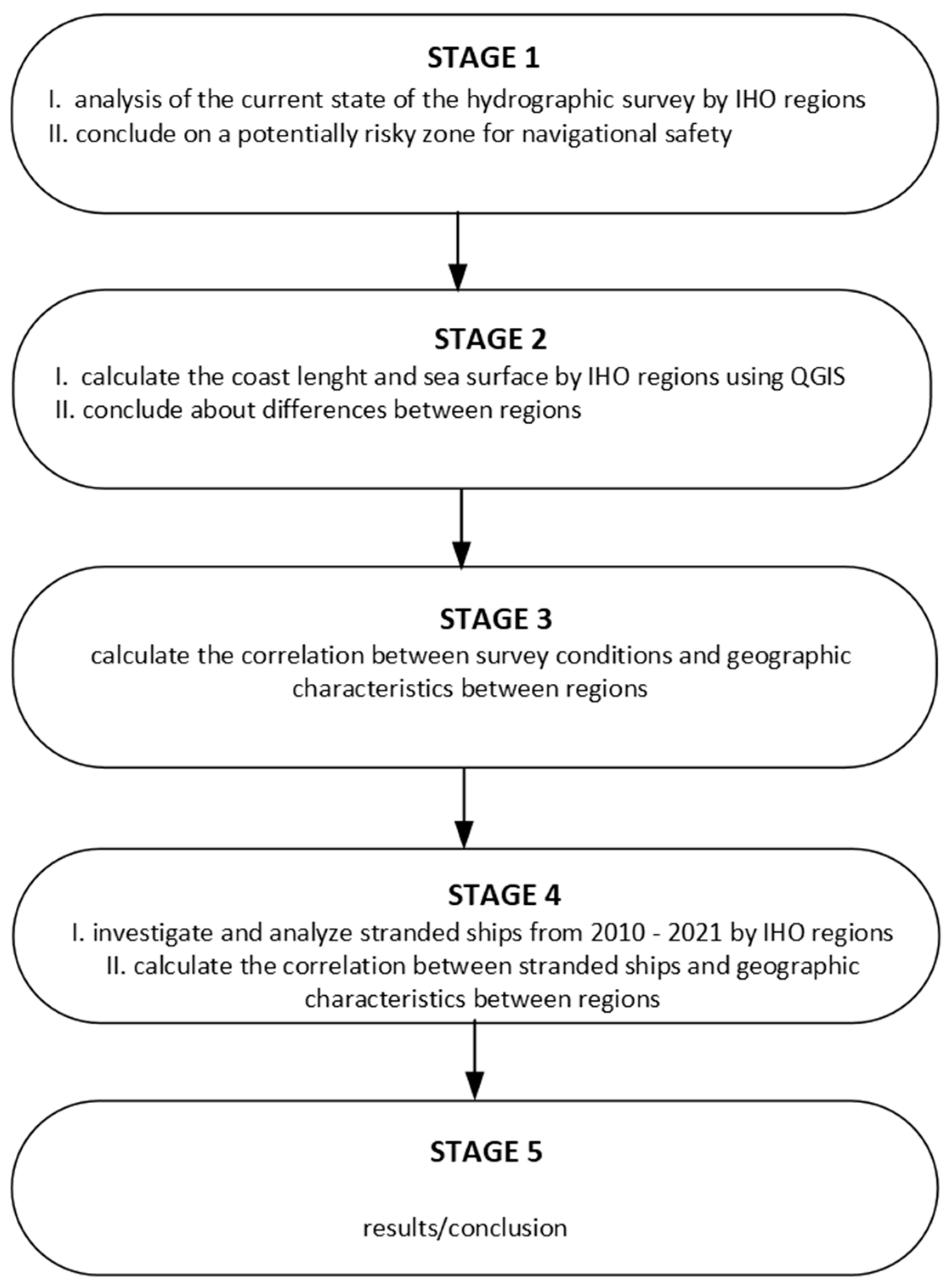
Figure 1. The integrated approach of determining potentially risky IHO regions.
Jmse 11 01498 g001
Figure 2. The procedure to obtain the status of the hydrographic survey by IHO regions.
Jmse 11 01498 g002
Figure 3. A general framework for QGIS.
Jmse 11 01498 g003
Figure 4. Model for calculating coastline length and sea surface by IHO region using QGIS.
Jmse 11 01498 g004
Figure 5. The status of implementation of the adequate hydrographic survey in world seas.
Jmse 11 01498 g005
Figure 6. The state of the hydrographic survey by IHO regions at depths up to 200 m.
Jmse 11 01498 g006
Figure 7. IHO regions with coastlines and boundaries made in QGIS.
Jmse 11 01498 g007
Figure 8. The relationship of the investigated parameters by IHO regions: (a) coastline length; (b) sea surface.
Jmse 11 01498 g008
Figure 9. Graphical representation of the stranded ships from 2010 to 2021 concerning IHO zones. (Note: The blue dots represent the actual values (Table 3) of the number of stranded ships, whereas the red line represents the values of the number of stranded ships after moving average filtering. Also, all graphs have the same y-axis.).
Jmse 11 01498 g009
Figure 10. Graphical representation between correlations of coastline length and sea surface concerning the number of stranded ships.
Jmse 11 01498 g010
Table 1. Strength of association for different ranges of the coefficient.
RangeStrength of Association
0No association
0 to ±0.25Negligible association
±0.25 to ±0.50Weak association
±0.50 to ±0.75Moderate association
±0.75 to ±1Very strong association
±1Perfect association
Table 2. Correlation matrix between attributes.
AttributesSea SurfaceCoastline LengthAdequate SurveyNeed to be ResurveyedUnsurveyInaccurate Data
Sea Surface10.146−0.516−0.3530.6310.408
Coastline Length 1−0.162−0.2990.3510.171
Adequate Survey 1−0.291−0.865−0.983
Need to be resurveyed 1−0.1980.358
Unsurvey 10.845
Inaccurate Data 1
Table 3. Sea surface, coast length for each IHO region, and maritime causalities from 2010 to 2021.
RegionsSea Surface (km2)Coast Length (NM)Number of Stranded Ship’s in IHO Regions through the Years
201020112012201320142015201620172018201920202021Total
A51,227,091.1179,87564843347010040
B17,593,21471,01252905528431044
C118,347,282.633,2852010210000118
C229,173,572.149,303110222201140025
D5,394,984.5756,47851281556135464083
E410,040.8534,17061257315212237
F2,986,455.3833,696157191215101395854122
G14,776,171.630,830824102135231041
H43,040,129.924,05203240033101017
I1,050,337.5511,73411121014120115
J22,245,978.846,37966121142000023
K40,773,776.2179,220111317144215214622111
L79,721,336.489,25642300112401119
M2,163,382,64529,5190000000000101
N1,246,495,013202,4141030100011007
Total3,736,618,0291,071,223815380704835607229351911593
Table 4. Establishing the relationships between the proposed variables.
The Number of Stranded Ships
201020112012201320142015201620172018201920202021Total
Coastline
Length
C
[%]
61.9767.4462.2965.1556.2958.0958.3758.1560.1252.2747.7332.0260.99
p-value0.0140.0060.0130.0090.0290.0230.0220.0230.0180.0460.0720.2450.016
Sea SurfaceC
[%]
18.2435.7532.5338.0023.2923.18−22.3210.6831.8992.2698.8384.8554.94
p-value0.5150.1910.2370.1620.4040.4060.4240.7050.2470.0000.0000.0000.034
Disclaimer/Publisher’s Note: The statements, opinions and data contained in all publications are solely those of the individual author(s) and contributor(s) and not of MDPI and/or the editor(s). MDPI and/or the editor(s) disclaim responsibility for any injury to people or property resulting from any ideas, methods, instructions or products referred to in the content.