Differing Aspects of Free and Bound Waves in Obtaining Orbital Velocities from Surface Wave Records

Abstract

In coastal zones, the accurate calculation of orbital particle velocities from surface wave measurements is quite important for estimating sediment transport, which is essentially controlled by the near-bottom velocity field. The main difficulty in obtaining orbital velocities from surface wave profiles is associated with the simultaneous existence of free and bound waves of the second harmonic with the same frequencies but different wave numbers. In a laboratory experiment, a discrepancy between the orbital velocities measured at different depths and the velocities obtained from synchronous wave records with the widely used transfer function of the linear theory was shown. The main reason for this was the different attenuations of free and bound waves with depth. Modeling with high spatial resolution made it possible to separate the free and bound waves and confirm this finding. It was found that free wave amplitudes decay with depth in exact accordance with the linear theory, while bound wave amplitudes decay much faster than the linear wave and Stokes theories predict. This difference and the unknown law of bound waves’ attenuation can lead to the inference of inaccurate orbital velocities from free surface elevations.

1. Introduction

Waves are among the main factors determining the dynamics of shelf and coastal zones. They can lead to coastal erosion and dangerous situations for maritime ships and coastal structures. Therefore, recently, all over the world, much attention has been paid to global monitoring measurements of wave fields using remote sensing, lidar and satellite technologies. However, simpler methods of wave measurement using pressure sensors and submerged current meters are widely used to solve local problems. According to the linear theory of waves, the measured velocities and pressure can be recalculated into free surface elevations and in relation to each other using the dispersion relation of the linear wave theory. This makes it possible, for example, to measure free surface elevations and, based on these, to obtain velocities at different depths. Of more practical interest is the determination of free surface elevations (waves) from pressure data, because pressure gauges are easier to install for measurements. As shown in [1,2], the reconstruction of free surface elevations from pressure for the main component of a wave spectrum can be undertaken with an error rate within 5%.

The accuracy with which records of orbital wave velocities are obtained from measured free surface elevations is very important since, as shown by recent studies, sediment transport in coastal zones is determined by the asymmetry of wave velocities [3,4]. There are many formulas for calculating sediment transport based on this concept. The most widely used is Bailard’s formula [5,6]. This concept was also applied in the modern Xbeach model [7]. However, as shown in [8], linear wave theory has significant limitations in terms of its application to waves at intermediate and shallow water depths. The influence of nonlinearity on the dispersion properties of these waves can be described only by a completely nonlinear model. During nonlinear wave transformations, multiple higher (mainly second) and lower (infragravity) wave harmonics arise. The generated second harmonic does not satisfy the dispersion relation of the linear theory. This leads to the simultaneous occurrence of waves with different wavenumbers at the same frequency. This paradox is known as the existence of free and bound waves [9,10,11]. In [2], it was revealed that the transfer function for obtaining the velocity records from free surface elevations for the second harmonics differs from the linear theory. This was attributed to the presence of free and bound waves. Experimental studies of the relationship between wave motions and orbital velocities at different depths, carried out under different conditions of wave transformation, have shown that linear theory as a whole can predict flow velocities to within about 7%. This discrepancy was explained by turbulence, which is not described by the linear theory [12].

As shown in [13], by applying the stochastic second-order wave model to assess the statistical properties of wave orbital velocity in random sea states below the water surface, sub-harmonics dominate the second-order contribution to orbital velocity. Furthermore, a substantial deviation of the upper and lower tails of the probability density function from the Gaussian distribution was noticed. Orbital velocities are faster under the wave trough and slower under the wave crest when compared with linear theory predictions. These results were also confirmed experimentally. These nonlinear effects have been shown to strengthen when reducing the water depth and to weaken with the broadening of the wave spectrum.

The deviation from the Gaussian statistics of the orbital wave velocities associated with nonlinearity was also noted in [14]. It was found that the histogram of instantaneous wave orbital velocities perfectly followed the Gaussian distribution, as commonly assumed, while the histogram of the wave orbital velocity’s amplitudes was less accurately described by the Rayleigh distribution.

There are variants of the nonlinear dispersion relation (most of which are based on modifications of the dispersion relation proposed in [15]) that could be used instead of the linear theory dispersion relation. However, there is no uniquely accepted form of nonlinear dispersion relation for obtaining an analytical transfer function between free surface elevations and orbital velocities. In general, nonlinear dispersion relations introduce nonlinear parameters, such as wave steepness (the ratio of amplitude to wavelength), into a formula. But, they also do not allow the calculation of two wavenumbers for the same frequency, i.e., the separation of free and bound waves.

There are two approaches to solving the problem. The first is empirical parametrization. In this way, for example, in modern models of sediment transport, the asymmetry of wave velocities on wave parameters is described. The most widely known and used parameterization is on the base of the Ursell number, representing the relationship between the nonlinear and the dispersion properties of waves (for example, [7,16,17]). As shown in many papers, this parameterization works well under some conditions of wave transformation and not very well under others, which leads to constant efforts to improve it (for example, [2,18,19,20]). The main disadvantage of this parametrization is the inability to take into account the fluctuations in the phase shift between the first and second nonlinear harmonics arising from the interference between free and bound second wave harmonics [21]. Therefore, the parametrization works satisfactorily only for long waves, whose wavelength is comparable to the width of the coastal zone and such fluctuations will be less expected.

The second approach is based on constructing and improving the accuracy of the transfer function using various wavenumber approximations that rely on a nonlinear wavenumber correction. In particular, it takes into account the contribution of the most energetic mode of the spectrum [22,23,24]. A nonlinear fully dispersive method for reconstructing the free surface elevation from pressure or wave orbital velocities measured under nonlinear waves in the coastal zone is proposed. This method is based on the knowledge of the dominant component of wavenumber spectra to account for varying amounts of forced energy at a particular frequency. It uses a Boussinesq approximation of the root mean square wave number suggested earlier in [22]. The accuracy of this reconstruction is directly dependent on that of the Boussinesq approximation for the considered water depths. It was noted that the relation between pressure, orbital velocity, and free surface elevations in nearshore nonlinear waves strongly depends on the relative input of bound components at high frequencies, making the ability to predict it, for example, through root mean square wave number, important. This approach is in good agreement with experimental data and therefore shows promise for further development. However, a detailed study of the contribution of free and bound wave components to velocities and pressure, from the point of view of their relations with free surface elevations and variation with depth, has not been carried out. Without such a study, the prospects and directions for improving the existing parametrizations will not be clear. Therefore, the main purpose of our paper is to study the relationship between free surface elevations and orbital velocity measurements at different distances from the bottom using the data from a laboratory experiment and numerical simulation to evaluate the contribution of free and bound waves.

This paper is organized as follows: Section 2 presents the descriptions of the laboratory experiment, numerical model, and methods of analysis. The results obtained from the analysis of experimental data (Section 3.1) and model data (Section 3.2) with their simultaneous discussion are presented in Section 3. Section 4 concludes this paper.

2. Experiments and Methods

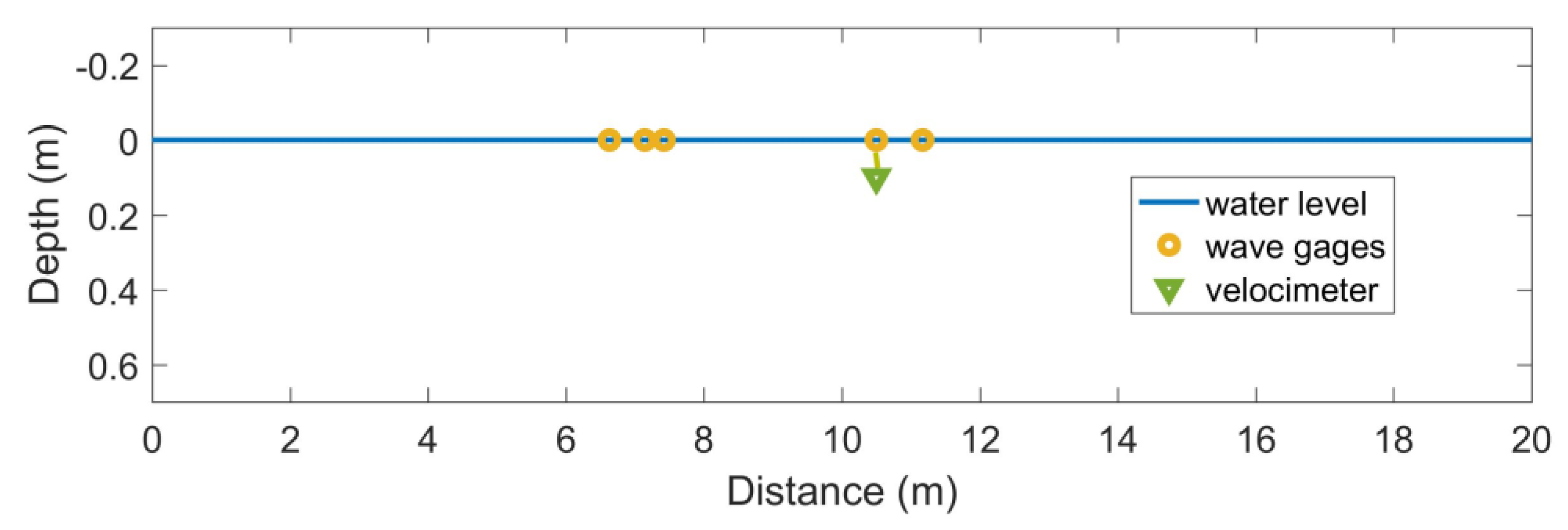
2.1. Laboratory Experiment

The laboratory experiment was conducted in the wave flume of the Coastal and Harbor Engineering Laboratory at Yildiz Technical University (Istanbul, Turkey). The two-dimensional flume has the following dimensions: 20 m in length, 1 m in width, and 1 m in depth. It is equipped with a fully controlled piston-type wave generator than includes an active wave absorption system and is capable of generating both regular and irregular waves. Waves measurements were taken using 4 capacity-type wave gauges with a sampling frequency of 200 Hz. To measure 3D water velocity fluctuations with sampling frequency of 100 Hz, a high-resolution acoustic velocimeter Vectrino (Nortek, Norway) was used. The Data Acquisition software (HR DAQ, HR Wallingford, United Kingdom) was used to collect the data from the wave gauges and velocimeter.

At a distance of 10.5 m from the wave generator, a wave gauge and Vectrino were installed together to measure surface waves and orbital velocities synchronously at various distances from the bottom. Data from both instruments were used for analysis. The experiment setup is depicted in Figure 1.

Only the horizontal velocity component (hereinafter referred to as velocity) was considered for the velocities. The choice was made because the asymmetry of horizontal velocities plays a crucial role in sediment transport in the coastal zone. Monochromatic waves were used as the experimental model waves. Detailed wave parameters and the distances from the bottom at which the velocities were recorded are provided in

Table 1. Wave parameters in laboratory experiment.

No	Amplitude (a), m	Period, s	Wave Number (k), 1/m	kH	ak	Ursell Number Ur = (ak)/(kH)3	Water Depth (H), m	Depths of Velocities Measurements (Distance from Bottom), m
1	0.15	2	1.36	0.95	0.20	0.237	0.7	0.35, 0.43, 0.45, 0.47, 0.49, 0.51, 0.53, 0.55, and 0.61
2	0.075	2	1.36	0.95	0.10	0.118	0.7	0.43, 0.45, 0.47, 0.49, 0.51, 0.53, 0.55, 0.61, and 0.63
3	0.15	1.3	2.53	1.77	0.38	0.069	0.7	0.43, 0.45, 0.47, 0.49, 0.51, 0.53, and 0.55
4	0.18	1	4.11	2.26	0.74	0.064	0.55	0.31, 0.33, 0.35, 0.37, 0.39, 0.41, 0.43, 0.45, and 0.47

.

2.2. Numerical Simulation

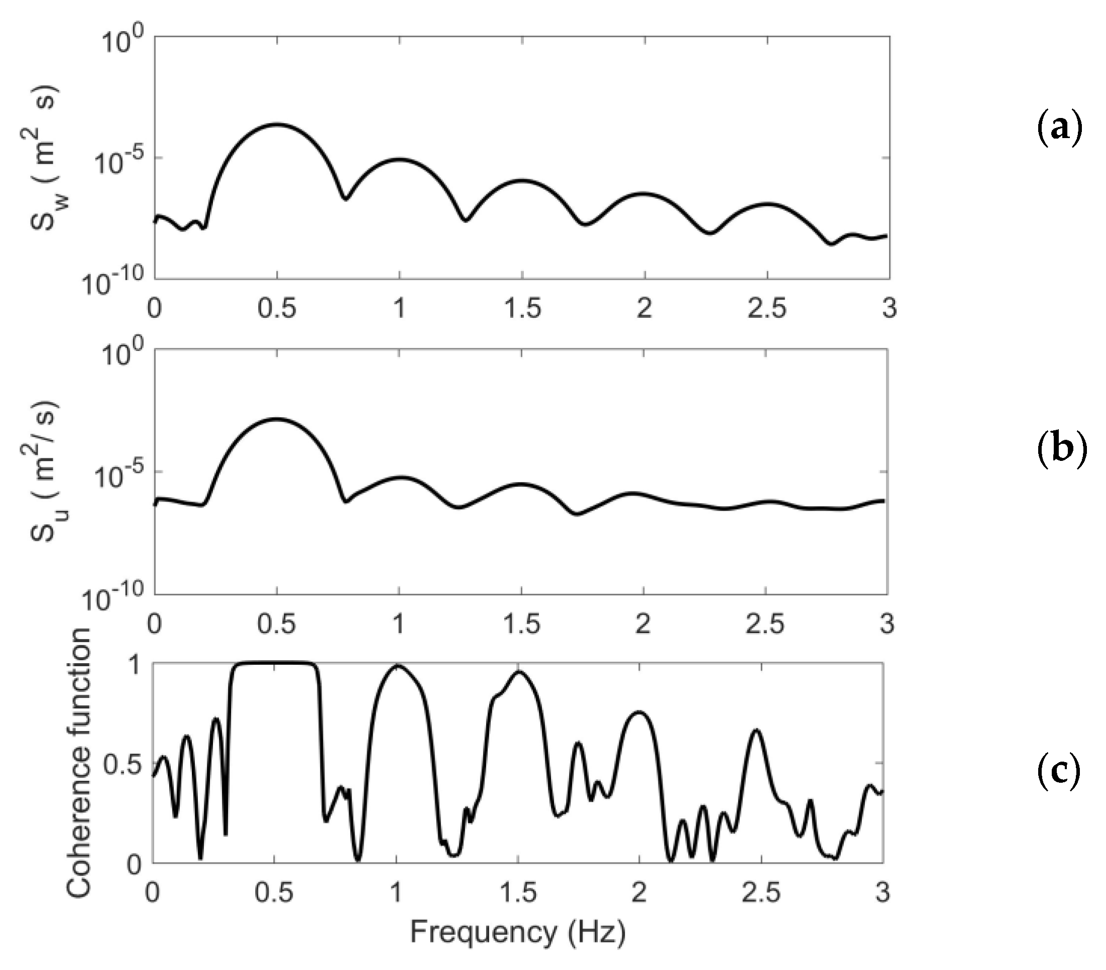
For a detailed study of the relationship between the free surface elevations and the velocity, a numerical simulation was carried out using the SWASH model with standard settings recommended by default [25].

SWASH (Simulating WAves till SHore) is an open-source phase-resolving fully nonlinear numerical model that is extensively utilized for simulating coastal and nearshore wave dynamics (http://swash.sourceforge.net/ (accessed on 23 July 2023)). It is based on the fully nonlinear shallow water equations, incorporating non-hydrostatic pressure effects and, by default, exploits the finite difference method on staggered Cartesian grids [26,27,28]. The model solves continuity and momentum equations, enabling it to reproduce unsteady and rotational flows, as well as nonlinear wave–wave interactions, including surf beat and triads. SWASH effectively accounts for wave propagation, frequency dispersion, shoaling, refraction, and diffraction.

SWASH has been validated to accurately reproduce crucial aspects of wave transformation dynamics. It successfully captures nonlinear shoaling [28,29], wave breaking [30], and wave runup [31]. Furthermore, it has been demonstrated that SWASH accurately represents nonlinear near-resonant interactions and bound wave interactions up to the 5th order [32,33]. The accuracy of the velocity modeling is discussed in [34], where the author shows good agreement between higher-order statistical moments simulated with the SWASH model and laboratory measurements in a wave flume.

The propagation of a monochromatic wave with an amplitude of 0.075 m and a period of 2 s (Test 2, Table 1) was simulated in a 30 m long numerical flume with a water depth of 0.7 m, with a spatial resolution of 0.1 m. The time step in the simulation was 0.05 s, and the free surface elevation and velocity data were output with a step of 0.1 s. Seven layers were specified in the model, so that the vertical points, where velocities were output synchronously with the free surface elevations at distances of 0.61, 0.43, 0.37, 0.21, and 0.11 m from the bottom, were in the middle of the model layers.

At the end of the numerical flume, in order to avoid the influence of reflection, the absorption condition (sponge layer) was set. In this simulation, no bottom friction or turbulent mixing was considered.

2.3. Data Analysis

The methods of spectral and cross-spectral analysis were utilized in this study. Pre-processing of the laboratory experiment’s time series involved linear filtering of frequencies above 3 Hz using the direct and inverse Fourier transform method to eliminate the influence of turbulence [35]. Additionally, linear filtering in the frequency and space domains was applied to the model data to extract free and bound wave chronograms.

The transfer function for recalculating the frequency components of the free surface elevations into velocity components was determined as the ratio of the velocity spectra to the wave spectra [2]:

$$G\left(f\right)=\sqrt{S_u\left(f\right)/S_w\left(f\right)}$$

(1)

where S_u and S_w represent velocity and wave spectrum, respectively, and f stands for frequency.

Since the spectrum values are proportional to the square of the amplitudes, this expression can be rewritten as follows:

$$G\left(f\right)=a_u\left(f\right)/a_w\left(f\right)$$

(2)

where a_u and a_w denote the amplitudes of velocity and wave calculated from spectra. In this study, only the amplitudes of the 1st and 2nd harmonics are considered.

The resulting transfer function for each nonlinear harmonic was compared with the theoretical transfer function obtained from the linear wave theory (for example, in [2]):

$$G_{lin}\left(f\right)=\omega \frac{\cos \mathrm{h}kz}{\sinh kH}$$

(3)

Or

$$a_{u lin}\left(f\right)=a_{w }\left(f\right)·G_{lin}\left(f\right)$$

where ω = 2πf represents angular frequency, k is the wavenumber, H is the water depth, and z is the distance from the bottom where velocity measurements were conducted. The wave number was calculated from the dispersion relation of the linear wave theory:

$${\omega }^2=gk·\tanh kH$$

(4)

where g denotes gravity acceleration.

To assess the relationship between the frequency components of the time series of free surface elevations and velocity at different depths, the coherence functions were constructed:

$$C\left(f\right)=\frac{{\left|S{\left(f\right)}_{wu}\right|}^2}{S{\left(f\right)}_{w}S{\left(f\right)}_u}$$

(5)

where S_wu represents cross-spectrum, S_u and S_w stand for velocity and wave spectra, respectively, and f is the frequency.

A coherence function value of one indicates that waves and velocities are completely related.

3. Results and Discussion

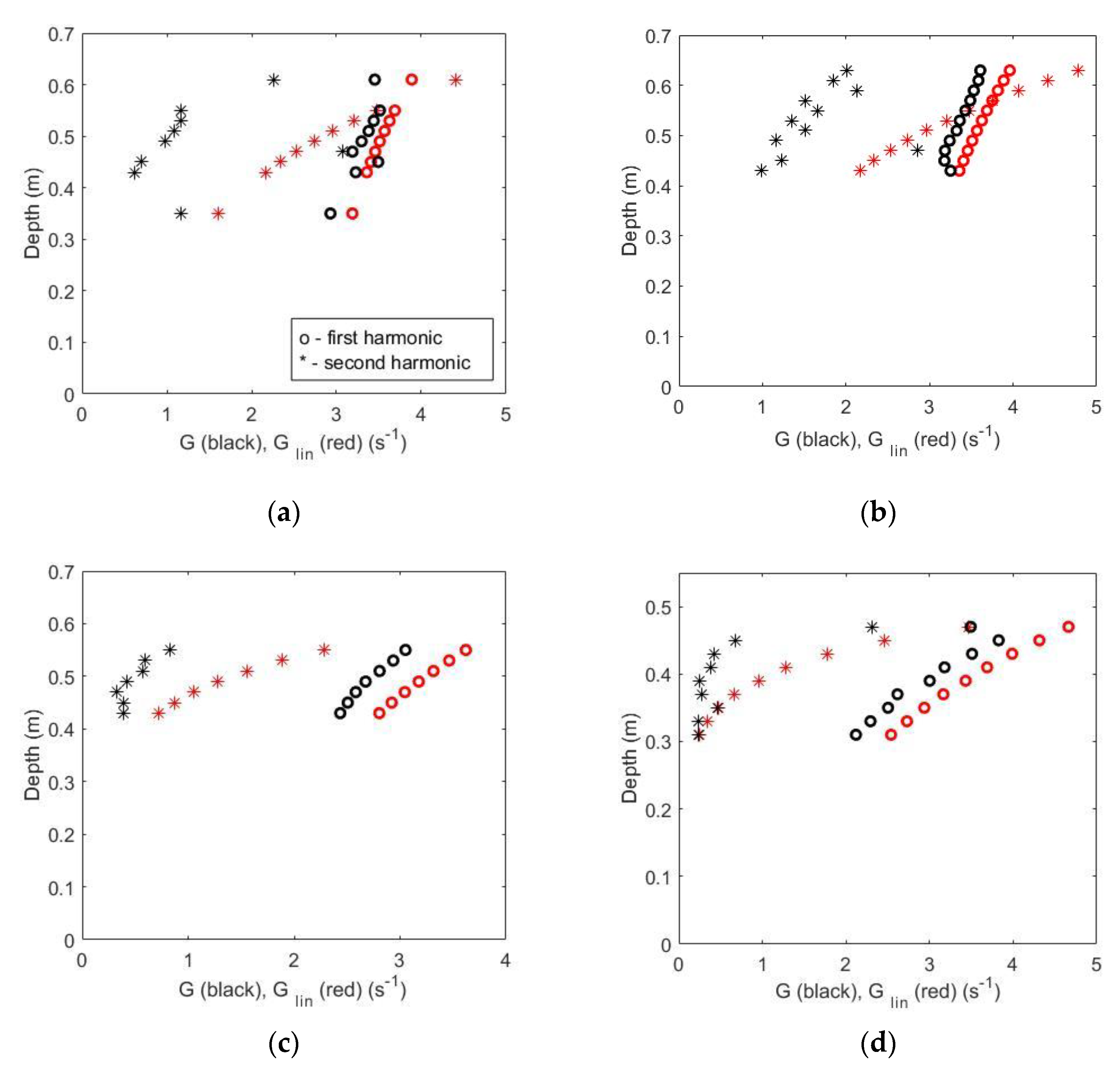
3.1. Laboratory Experiment

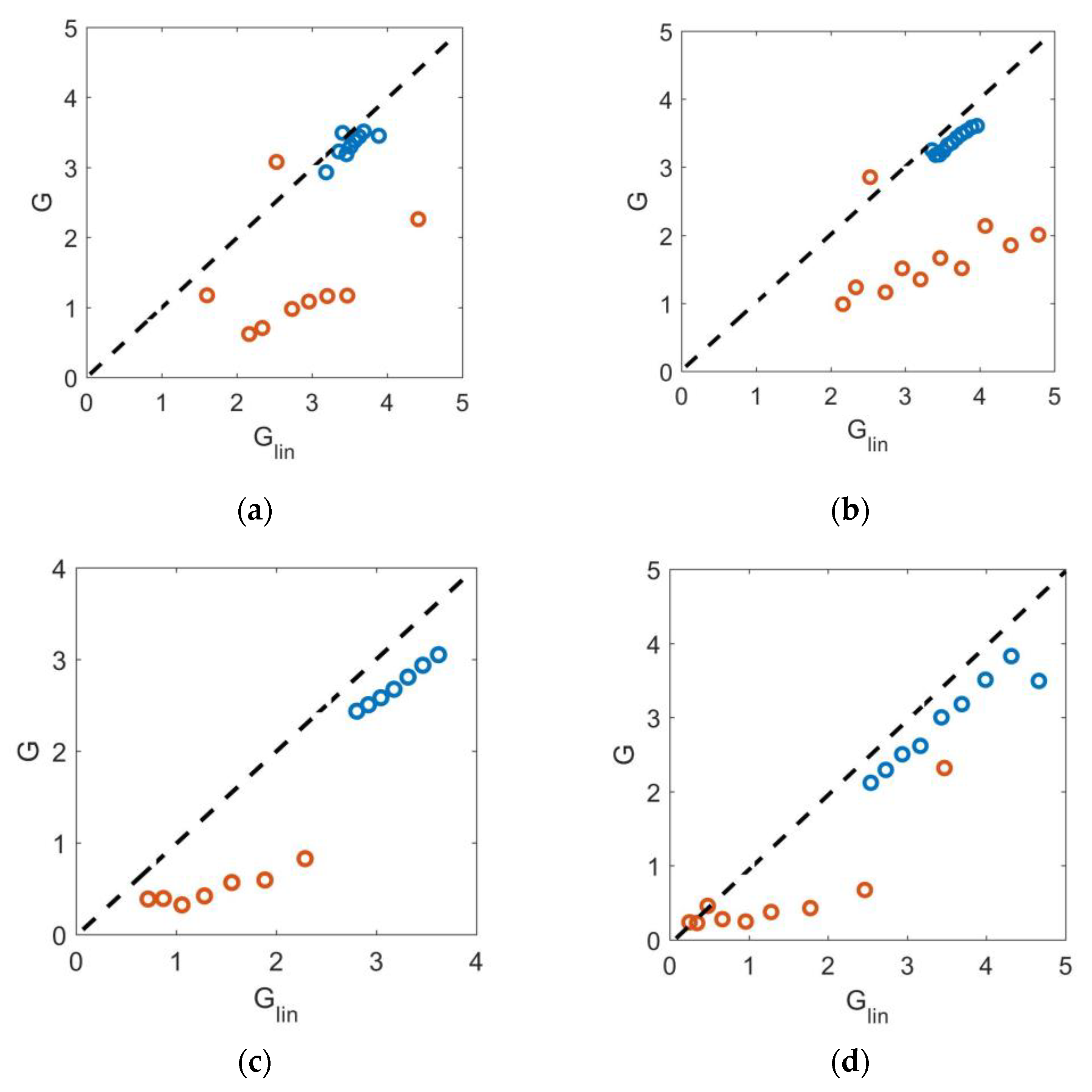
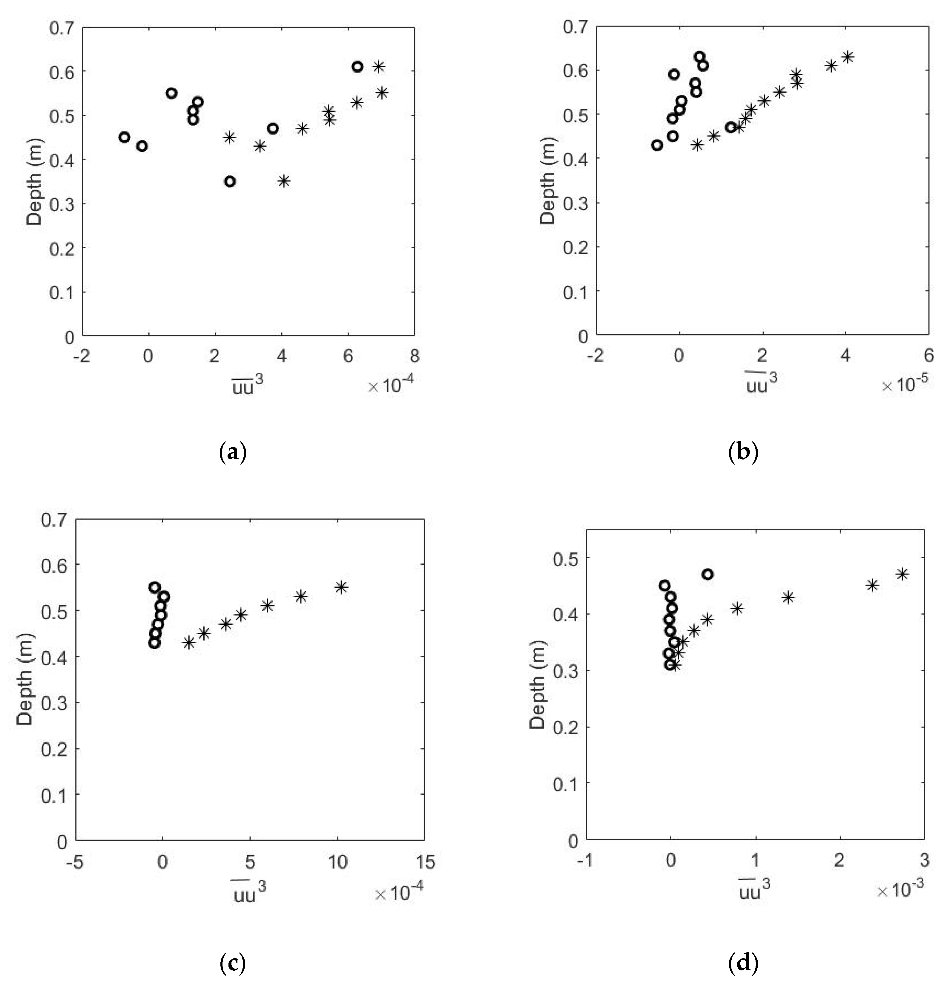
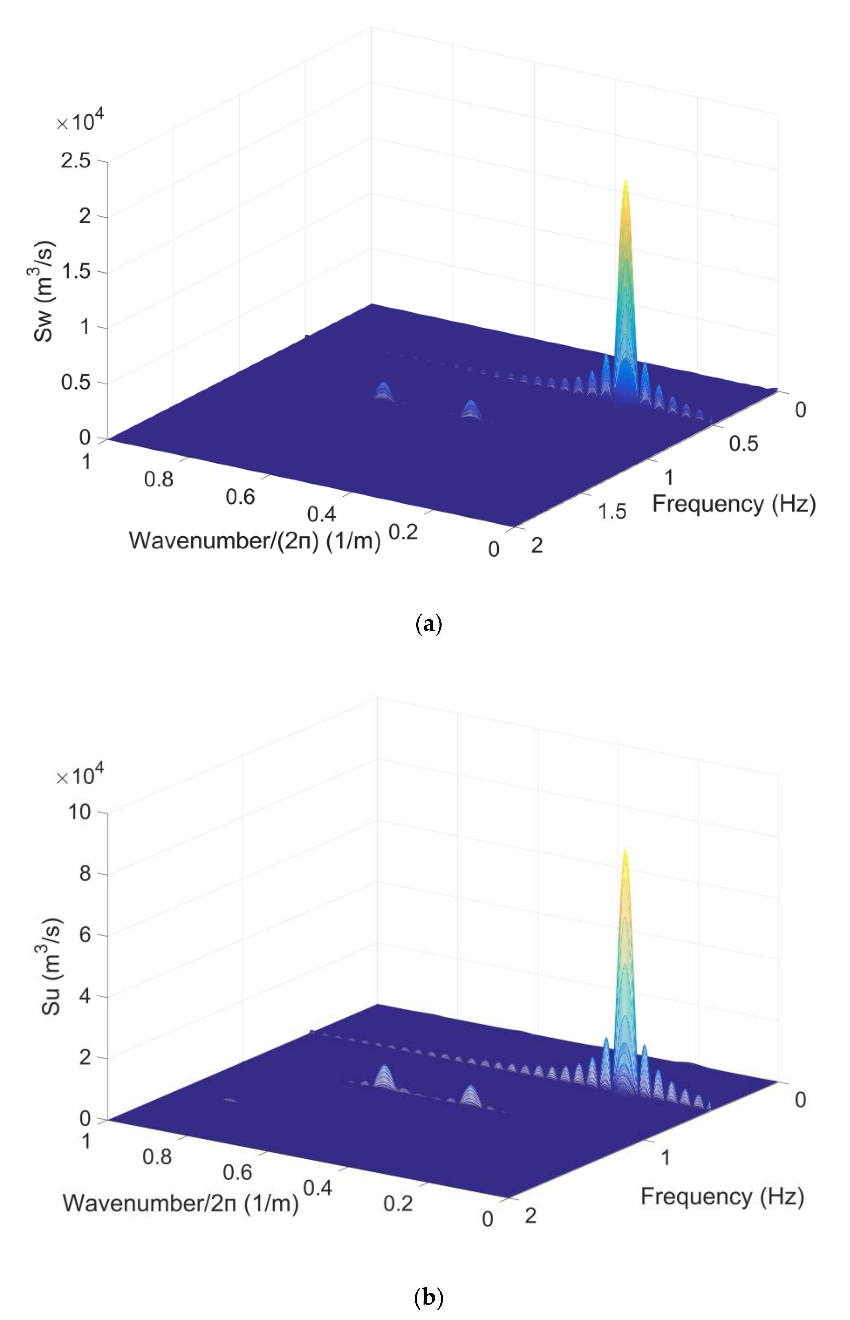
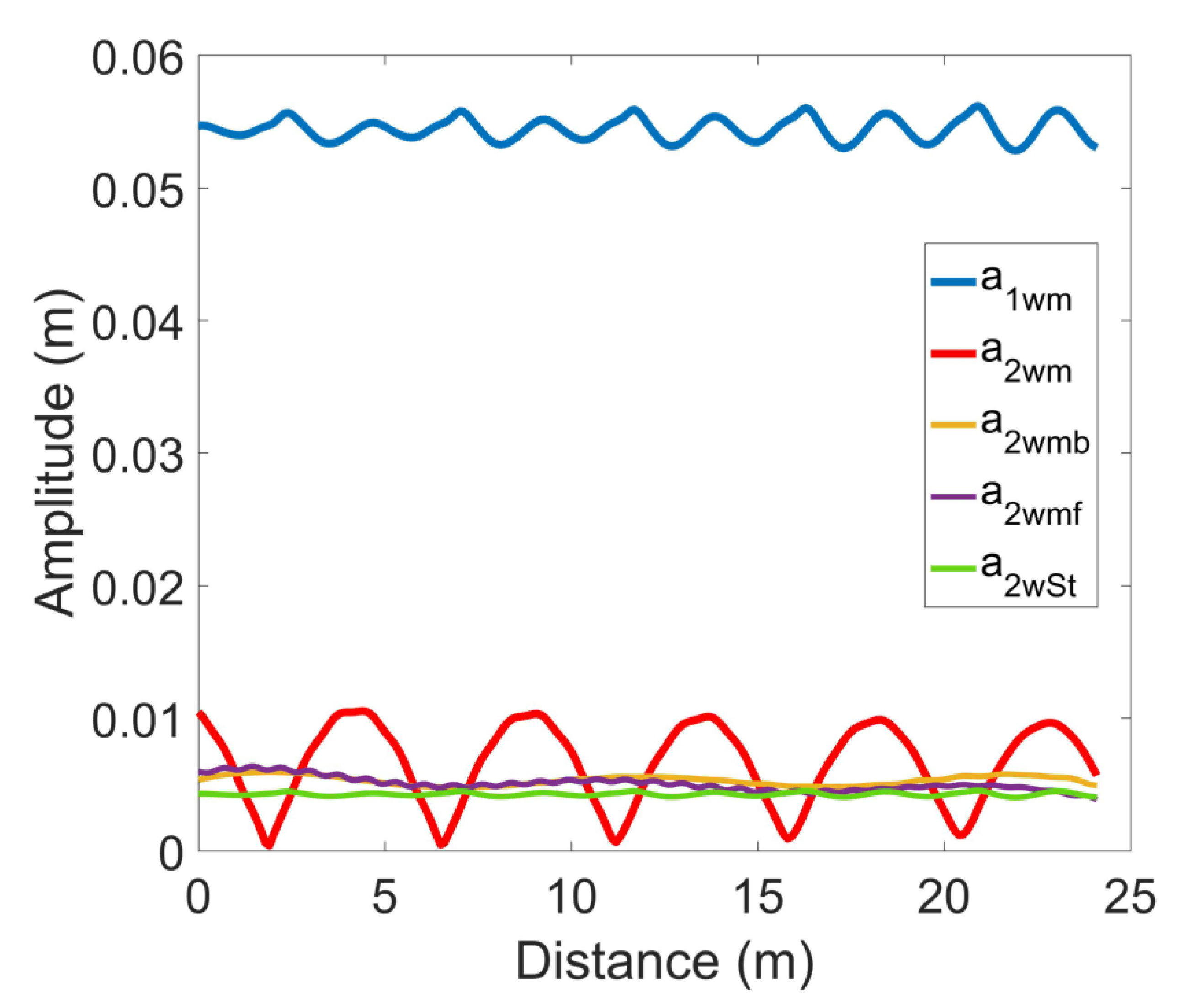
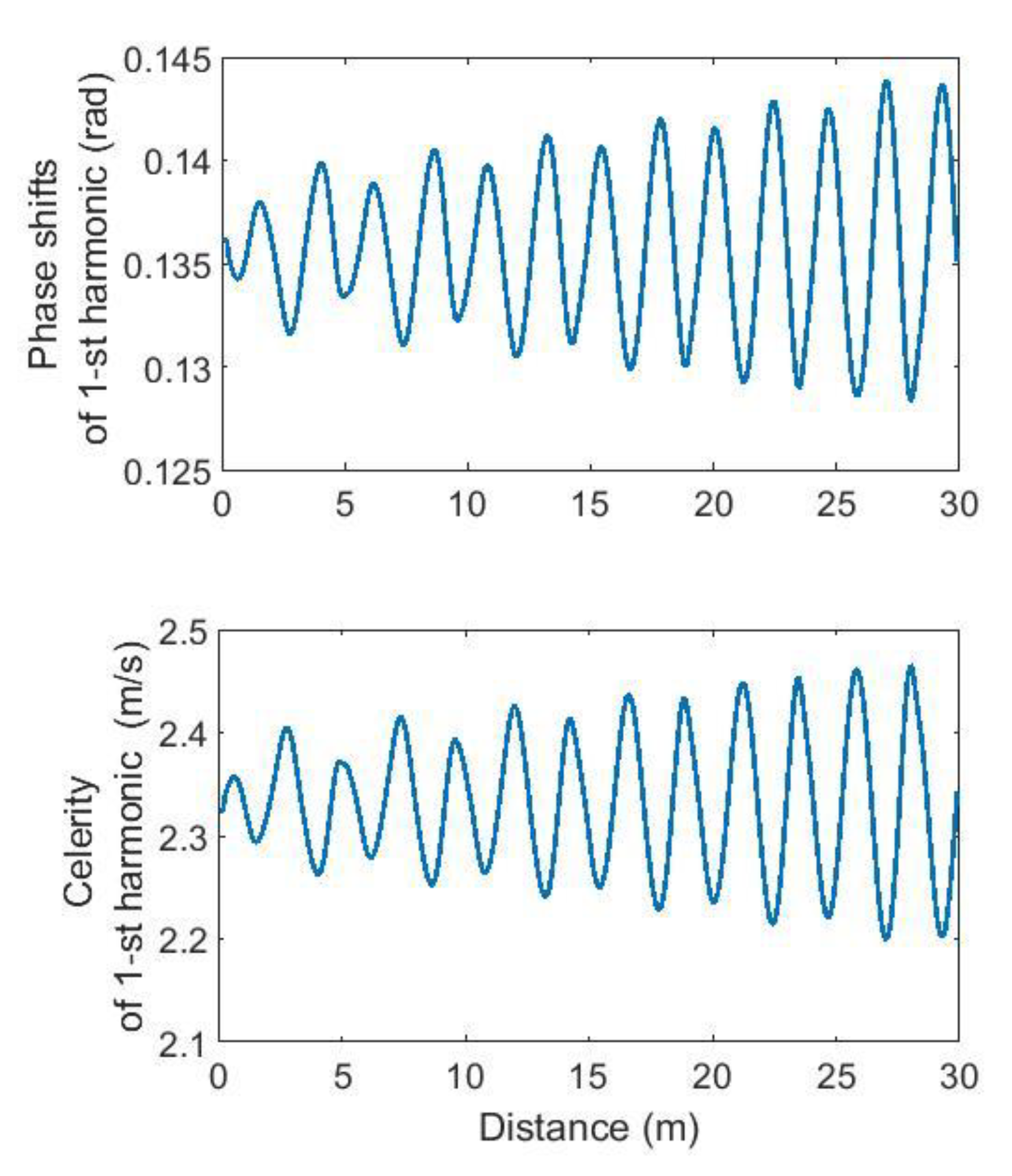
As indicated by the analysis of the experimental data, the wave transformation exhibits nonlinear behavior, leading to the formation of multiple nonlinear harmonics. These harmonics are clearly observable in both the wave and velocity spectra, which were constructed using the Welch method with a Hamming window [36] for all the experimental data at the specified depths.

Figure 2a,b present a typical example of such spectra for waves with an amplitude of 0.15 m and a period of 2 s at a depth of 0.51 m from the bottom. The coherence function showed a high value (approximately 1) at the main frequency of 0.5 Hz and the frequencies of the second and third multiple wave harmonics, which were 1 and 1.5 Hz, respectively. This high coherence value indicates that changes in the waves on the surface and velocities at different depths for these frequencies occur synchronously (Figure 2c). In the experimental data, as the distance from the surface increased, the value of the coherence function for the third nonlinear harmonic in short waves (Test 1 and Test 3, Table 1) significantly decreased due to its very small amplitude and rapid decay with depth. Conversely, for the second harmonics, the coherence function remained no lower than 0.8 in all cases. Consequently, we will focus our analysis on the first and second nonlinear harmonics.

The transfer function for the first and second nonlinear harmonics calculated from the experimental data using Formula (2) for all laboratory tests is shown in Figure 3. When comparing the obtained transfer function with the transfer function of the linear wave theory, it can be seen that for the main (first) harmonic, the values are generally close, and the difference does not exceed 17 percent. The difference can be attributed to the influence of the flume walls and bottom friction and measurement errors.

The situation is different for the second harmonics. In most cases, the values of the transfer function are significantly lower (by 40–70%) than those predicted by the linear theory. However, in some cases, the difference between the coefficient determined in the experiment and the linear theory does not exceed 20%.

Inaccuracies in velocity data obtained from wave measurements can significantly impact velocity asymmetry estimates. This error becomes evident when comparing the measured higher statistical moments of velocity with those obtained from wave records according to the linear theory.

Asymmetry can be defined in multiple ways. The first approach considers asymmetry in the time series of measured velocities, where it refers to the asymmetry with respect to the vertical and horizontal axes in the chronogram values. Another method involves calculating higher-order statistical moments (second, third, fourth, etc.) and examining the deviations of their values from 0 and 1, or estimating changes in the sign of the statical moment based on the measured chronogram. The higher-order statistical odd and even moments determine the asymmetry and skewness of velocities, respectively, and can be mathematically calculated as $\overline{u{u}^n}$, where the upper line denotes time averaging, and n = 1, 2, 3, 4, and so on. The value of n determines the order of the moment—first, second, third, etc. For instance, the second and third moments are included in the Bailard’s formula [3].

Figure 4 illustrates changes in the third velocity moment $\overline{u{u}^3}$, which is responsible for the transport of suspended sediments at different depths.

The potential impact of free and bound waves on the mismatch with the transfer function of the linear theory was mentioned in [2]. For irregular waves, they also obtained values for the second harmonics that not only coincided with those predicted by the linear theory, but were also significantly lower. However, no detailed study has been conducted in this matter. When considering the change in the measured transfer function with depth and comparing it with the transfer function of the linear theory, it becomes apparent that the decrease (attenuation) in the first harmonics occurs almost in accordance with the linear theory, while the transfer function for the second harmonics exhibits a completely different damping, in most cases faster than that predicted by the linear theory (Figure 5). Notably, as the distance from the surface increases, the change in the measured transfer function closely resembles the linear theory for Tests 3 and 4, where the waves are much shorter. In contrast, for Tests 1 and 2, where the waves are longer, a few values close to the transfer function of the linear theory are observed regardless of depth. The presence of different attenuation tendencies resembling and differing from the linear theory provides further support for the hypothesis about the influence of free and bound waves. These waves, characterized by different wavenumbers, are expected to have different transfer functions and amplitude attenuation with depth.

To study the influence of free and bound waves in detail, measurement data with good spatial resolution are needed. However, collecting such data is not easy in practice, even under laboratory conditions, due to the limited length of the wave flumes and the number of measuring instruments. Therefore, we will use simulation data to conduct a detailed analysis.

3.2. Modeling

A numerical simulation of wave propagation in the flume was performed using the SWASH model. The initial wave conditions in the modeling corresponded to Test 2 in the laboratory experiment described in Section 2. As a result of the simulation, the matrices of free surface elevations W(x,t) and horizontal components of the velocity of water particles u(z,x,t) were obtained at the following distances from the bottom: at z = 0.61 m, 0.43 m, 0.37 m, 0.21 m, and 0.11 m. Let us consider the wave harmonics present in the frequency and spatial (in terms of wave number) spectrum of waves.

Two-dimensional k-f spectra (in terms of frequencies f and wavenumbers k) of free surface elevations and velocities were calculated using the two-dimensional Fourier transform with the MATLAB function fft2. This function first calculates the one-dimensional Fourier transform of each column and then the one-dimensional Fourier transform of each row of the previous result without additional averaging over frequencies and wavenumbers. The width of the spectrum peaks was determined by the sizes of the temporal and spatial windows of 300 s and 30 m, respectively. The calculated spectra are shown in Figure 6.

The k-f spectrum is symmetric with respect to the origin. It shows a positive direction of wave energy propagation in positive wavenumber quadrants and positive and negative frequencies, while in the negative wavenumber quadrants, it shows a negative direction of wave energy propagation (or reflected wave energy). In our case, the energy of the reflected waves was equals to zero, and therefore only one quadrant is shown in the figures.

The k-f spectra clearly show the peak of the first harmonic at a frequency of 0.5 Hz with a wavenumber divided by 2π of 0.215 1/m. Two peaks of the second harmonic are also visible, corresponding to free and bound waves, with the same frequency of 1 Hz and wave numbers divided by 2π 0.43 1/m (bound second harmonic, with a wave number equal to twice the wave number of the first harmonic) and 0.647 1/m (free second harmonic, with a wave number satisfying the linear dispersion relation). The side lobes visible at the frequency of the first harmonic in the direction of the wavenumber axis are a consequence of using a rectangular spatial window in the calculation of the spectrum. In the analyzed case, the window is 30 m of a numerical flume.

According to [11], there should be a small peak of the bound first harmonic in the spectrum. However, for the conditions of our numerical simulation, the magnitude of this peak is small, and it is not visible against the background of side lobes. Nevertheless, these bound first harmonic waves are important because they explain the slight fluctuations with the frequency of the difference between the frequencies of the free and bound harmonics in the wave energy and transfer functions. This will be discussed below.

The velocity spectra at all depths have a form similar to the wave spectrum. The coherence functions between free surface elevations and velocity are equal to 1 at all frequencies. The calculated phase spectra demonstrate the absence of a phase shift between free surface elevations and velocities. High coherence and synchronous fluctuations in waves and velocities in the model data enable the construction of the transfer function as the real function based on the change in the amplitudes of harmonics with depth.

To examine the spatial fluctuations of free and bound wave components, as well as their first and second harmonics, we filtered the matrices of free surface elevations (rows—changes in space; columns—changes in time) and matrices of horizontal velocities into three separate matrices: one for the first harmonic and two for free and bound waves of the second harmonic, using direct and inverse Fourier transform. In the first step, each column was filtered into the first and second harmonics in the frequency domain, and then each row of the second harmonic matrices was filtered into free and bound components in the wavenumber domain. After that, the spatial changes in the amplitudes of the first and second frequency harmonics, as well as the free and bound waves of the second harmonic, were determined as the standard deviation of each column of the corresponding matrix multiplied by the square root of 2.

Let us compare amplitude changes with those predicted by the linear theory of waves and by the nonlinear theory of Stokes waves, including both linear and bound harmonics. Since the model waves have an Ursell number less than 1 (Table 1, Test 2), their comparison with the Stokes waves is quite appropriate. The relationship between free surface elevations (W) and the horizontal velocity component of water particles (u) in the second Stokes approximation at finite depth is defined in [37]:

$$\mathrm{W}\left(x,t\right)=a\cos \left(kx-\omega t\right)+\frac{1}{4}{a}^{2}k\frac{\cosh \left(kH\right)}{{\sinh }^3\left(kH\right)}\left(2+\cosh \left(2kH\right)\right)\cos \left(2kx-2\omega t\right)$$

(6)

$$u\left(z,x,t\right)=a\omega \frac{\cos \mathrm{h}kz}{\sinh kH}\cos \left(kx-\omega t\right)+\frac{3}{4}{a}^2\frac{\cosh \left(2kz\right)}{{\sinh }^4\left(kH\right)}\cos \left(2kx-2\omega t\right)$$

(7)

where a—amplitudes of wave harmonics calculated from wave spectrum, ω = 2πf—angular frequency, k—wavenumber, H—water depth, and z—distance from bottom where the modeled velocities were derived.

The first term in Equation (7) completely corresponds to the transfer function of the linear theory (3).

Figure 7 illustrates the changes in the amplitudes of the first and second harmonics of unseparated waves (selected from the frequency spectrum), which are further divided into free and bound second harmonics (selected from the k-f spectrum) and the amplitude of the second harmonic according to the second-order Stokes approximation (Equation (6)). It can be observed that the amplitudes of the first and unseparated second frequency harmonics fluctuate periodically. These fluctuations have been observed in various research papers and are also observed in nature (e.g., [10,11,38]). The evolution of the second harmonics, divided into free and bound components, indicates that they have nearly equal amplitudes that closely resemble the amplitude of the Stokes waves and remain practically unchanged in space.

To explain the observed spatial fluctuations in the energy of the first harmonic (blue line in Figure 7) with a characteristic length of 2.33 m, which exactly coincided with the wavelength of the second bound harmonic (wave number divided by 2π is 0.43, Figure 6), the process of nonlinear evolution of the first harmonic was considered in more detail. According to the fundamental law of conservation, the wave energy flux must be preserved during wave propagation in space. Therefore, the observed fluctuations in the amplitude of the first harmonic should be compensated by fluctuations in the energy transfer velocity. To check this, we calculated the phase velocities of the first harmonics from the phase shift between the waves of the first harmonic at neighboring simulation points.

The phase shift was calculated as

$$\mathsf{\Delta }\phi =arctan\frac{Imag\left(A_{ij}\right)}{Real\left(A_{ij}\right)},$$

(8)

where $A_{ij}=A_i{A}_j^{*}$, $A_i$, and $A_j^{}$ represent Fourier coefficients in neighboring by distance points i and j. The asterisk denotes the complex conjugate.

The “instantaneous” wave number was determined from the phase shift, and then the celerity was calculated as the ratio of the frequency that does not change in space to the instantaneous wave number. The obtained values are shown in Figure 8. As can be seen from Figure 7 and Figure 8, spatially periodic changes in the phase velocities and amplitudes of the first harmonics are uniquely related and have the same periodicity. Since the period does not change, these fluctuations indicate spatial fluctuations in the wavelength of the first harmonic, occurring due to nonlinear processes.

In Figure 9, the ratio of the model amplitude of the first velocity harmonic to the amplitude determined from the transfer function of the linear theory (3) is shown. It can be observed that both in the model data and the laboratory experiment, the change in the first harmonic with depth follows the predictions of the linear theory. Small spatial fluctuations of the ratio around 1 are caused by the wavelength fluctuation described above (Figure 7, Figure 8 and Figure 9). Furthermore, the change in the second free harmonic also aligns with the predictions of the linear theory (Figure 10).

Regarding the bound second harmonic, the transfer function deviates from the linear theory (Figure 11). The amplitude of the second bound harmonic decays more rapidly with depth. When comparing its decay rate with the amplitude predicted by the second-order Stokes approximation (the second terms on the right-hand side of Expressions (6) and (7)), it becomes evident that the associated harmonic also decays faster with depth. In other words, the transfer function cannot be derived from the Stokes approximation (Figure 12).

Thus, it is shown that the simultaneous existence of free and bound waves, along with the difference in the laws of their damping and the unknown law of damping of bound harmonics with depth, can be the reason for the inaccurate obtaining of velocities at different depths from the free surface elevations. However, by taking into account the damping of higher harmonics with depth, their contribution to the reconstructed velocities will decrease, making it possible to use the linear theory to describe the velocity field near the bottom. It should be noted that in the case of restoring the free surface elevations from the pressure records at the bottom using the linear wave theory, large errors can occur due to ignorance of the attenuation law of bound waves and neglect of the joint contribution of free and bound waves. To accurately convert free surface elevations into velocity, pressure, and vice versa, further development of a completely nonlinear theory of waves at a finite depth is necessary.

4. Conclusions

Based on laboratory experiments and numerical simulations using the SWASH model, it is evident that the presence of free and bound waves makes it challenging to accurately reconstruct velocities from the free surface elevations, especially near the surface, due to the different laws of attenuation of their amplitudes with depth. The damping law of bound waves remains unknown, necessitating further development of a completely nonlinear theory of waves at a finite depth in order to find an analytical solution or approximation. Additionally, the transfer function also exhibits spatial fluctuations related to changes in the wave number due to nonlinear processes.

References

1. Bishop, C.T.; Donelan, M.A. Measuring waves with pressure transducers. Coast. Eng. 1987, 11, 309–328. [Google Scholar] [CrossRef]
2. Herbers, T.H.C.; Lowe, R.L.; Guza, R.T. Field observations of orbital velocities and pressure in weakly nonlinear surface gravity waves. J. Fluid Mech. 1992, 245, 413–435. [Google Scholar] [CrossRef]
3. Bailard, J. An energetics total load sediment transport model for a plane sloping beach. J. Geophys. Res. 1981, 86, 10938–10954. [Google Scholar] [CrossRef]
4. Saprykina, Y. The Influence of Wave Nonlinearity on Cross-Shore Sediment Transport in Coastal Zone: Experimental Investigations. Appl. Sci. 2020, 10, 4087. [Google Scholar] [CrossRef]
5. Camenen, B.; Larroudé, P. Comparison of sediment transport formulae for the coastal environment. Coast. Eng. 2003, 48, 111–132. [Google Scholar] [CrossRef] [Green Version]
6. Abreu, T.; Silva, P.A.; Sancho, F.; Temperville, A. Analytical approximate wave form for asymmetric waves. Coast. Eng. 2010, 57, 656–667. [Google Scholar] [CrossRef]
7. Ruessink, B.G.; Ramaekers, G.; van Rijn, L.C. On the parameterization of the free-stream non-linear wave orbital motion in nearshore morphodynamic models. Coast. Eng. 2012, 65, 56–63. [Google Scholar] [CrossRef]
8. Shugan, I.; Kuznetsov, S.; Saprykina, Y.; Chen, Y.-Y. Physics of Traveling Waves in Shallow Water Environment. Water 2021, 13, 2990. [Google Scholar] [CrossRef]
9. Hasselmann, K. On the nonlinear energy transfer in a gravity-wave spectrum. Part 1. General theory. J. Fluid Mech. 1962, 12, 481–500. [Google Scholar] [CrossRef]
10. Madsen, P.A.; Sørensen, O.R. Bound waves and triad interactions in shallow water. Ocean. Eng. 1993, 20, 359–388. [Google Scholar] [CrossRef]
11. Kuznetsov, S.; Saprykina, Y. Nonlinear Wave Transformation in Coastal Zone: Free and Bound Waves. Fluids 2021, 6, 347. [Google Scholar] [CrossRef]
12. Drennan, W.M.; Kahma, K.K.; Donelan, M.A. The velocity field beneath wind-waves—Observations and inferences. Coast. Eng. 1992, 18, 111–136. [Google Scholar] [CrossRef]
13. Alberello, A.; Chabchoub, A.; Gramstad, O.; Babanin, A.; Toffoli, A. Non-Gaussian properties of second-order wave orbital velocity. Coast. Eng. 2016, 110, 42–49. [Google Scholar] [CrossRef] [Green Version]
14. You, Z.-J. The statistical distribution of near bed wave orbital velocity in intermediate coastal water depth. Coast. Eng. 2009, 56, 844–852. [Google Scholar] [CrossRef]
15. Kirby, J.T.; Dalrymple, R.A. An approximate model for nonlinear dispersion in monochromatic wave propagation models. Coast. Eng. 1996, 9, 545–561. [Google Scholar] [CrossRef]
16. Doering, J.C.; Bowen, A.J. Parametrization of orbital velocity asymmetries of shoaling and breaking waves using bispectral analysis. Coast. Eng. 1995, 26, 15–33. [Google Scholar] [CrossRef]
17. Elfrink, B.; Hanes, D.; Ruessink, B.G. Parameterization and simulation of near bed orbital velocities under irregular waves in shallow water. Coast. Eng. 2006, 53, 915–927. [Google Scholar] [CrossRef]
18. Rocha, M.V.L.; Michallet, H.; Silva, P.A. Improving the parameterization of wave nonlinearities—The importance of wave steepness, spectral bandwidth and beach slope. Coast. Eng. 2017, 121, 77–89. [Google Scholar] [CrossRef]
19. Nam, P.T.; Staneva, J.; Thao, N.T.; Larson, M. Improved Calculation of Nonlinear Near-Bed Wave Orbital Velocity in Shallow Water: Validation against Laboratory and Field Data. J. Mar. Sci. Eng. 2020, 8, 81. [Google Scholar] [CrossRef] [Green Version]
20. Malarkey, J.; Davies, A.G. Free-stream velocity descriptions under waves with skewness and asymmetry. Coast. Eng. 2012, 68, 78–95. [Google Scholar] [CrossRef]
21. Saprykina, Y.V.; Shtremel, M.N.; Kuznetsov, S.Y. On the possibility of biphase parametrization for wave transformation in the coastal zone. Oceanology 2017, 57, 253–264. [Google Scholar] [CrossRef]
22. Herbers, T.H.C.; Elgar, S.; Sarap, N.A.; Guza, R.T. Nonlinear dispersion of surface gravity waves in shallow water. J. Phys. Oceanogr. 2002, 32, 1181–1193. [Google Scholar] [CrossRef]
23. Martins, K.; Bonneton, P.; Lannes, D.; Michallet, D. Relationship between Orbital Velocities, Pressure, and Surface Elevation in Nonlinear Nearshore Water Waves. J. Phys. Oceanogr. 2021, 51, 3539–3556. [Google Scholar] [CrossRef]
24. Martins, K.; Bonneton, P.; de Viron, O.; Turner, I.L.; Harley, M.D.; Splinter, K. New Perspectives for Nonlinear Depth-Inversion of the Nearshore Using Boussinesq Theory. Geophys. Res. Lett. 2023, 50, 1944–8007. [Google Scholar] [CrossRef]
25. SWASH. Available online: http://swash.sourceforge.net/download/zip/swashuse.pdf (accessed on 14 April 2023).
26. Stelling, G.; Zijlema, M. An accurate and efficient finite-difference algorithm for non-hydrostatic free-surface flow with application to wave propagation. Int. J. Numer. Meth. Fluids 2003, 43, 1–23. [Google Scholar] [CrossRef]
27. Zijlema, M.; Stelling, G.S. Further experiences with computing non-hydrostatic free-surface flows involving water waves. Int. J. Numer. Meth. Fluids 2005, 48, 169–197. [Google Scholar] [CrossRef]
28. Zijlema, M.; Stelling, G.; Smit, P. SWASH: An operational public domain code for simulating wave fields and rapidly varied flows in coastal waters. Coast. Eng. 2011, 58, 992–1012. [Google Scholar] [CrossRef]
29. Van Vledder, G.P.; Ruessink, G.; Rijnsdorp, D.P. Individual wave height distributions in the coastal zone: Measurements and simulations and the effect of directional spreading. In Proceedings of the 7th International Conference on Coastal Dynamics, Arcachon, France, 24–28 June 2013. [Google Scholar]
30. Stelling, G.S.; Zijlema, M. Numerical modeling of wave propagation, breaking and run-up on a beach. Lect. Notes Comput. Sci. Eng. 2009, 71, 373–401. [Google Scholar]
31. Guimarães, P.V.; Farina, L.; Toldo, E., Jr.; Diaz-Hernandez, G.; Akhmatskaya, E. Numerical simulation of extreme wave runup during storm events in Tramanda Beach, Rio Grande do Sul, Brazil. Coast. Eng. 2015, 95, 171–180. [Google Scholar] [CrossRef] [Green Version]
32. Rijnsdorp, D.P.; Smit, P.B.; Zijlema, M.; Reniers, A.J.H.M. Efficient non-hydrostatic modelling of 3D wave-induced currents using a subgrid approach. Ocean Model. 2017, 116, 118–133. [Google Scholar] [CrossRef] [Green Version]
33. Vyzikas, T.; Stagonas, D.; Maisondieu, C.; Greaves, D. Intercomparison of Three Open-Source Numerical Flumes for the Surface Dynamics of Steep Focused Wave Groups. Fluids 2021, 6, 9. [Google Scholar] [CrossRef]
34. Xiaomin, L. Cross-Shore Velocity Moments in the Nearshore: Validating SWASH. TU Delft. 2015. Available online: http://resolver.tudelft.nl/uuid:6d64b611-7b9e-4235-ad57-a638188116b1 (accessed on 31 May 2023).
35. Kuznetsov, S.Y.; Saprykina, Y.V.; Dulov, V.A.; Chukharev, A.M. Turbulence Induced by Storm Waves on Deep Water. Phys. Oceanogr. 2014, 5, 22–31. [Google Scholar] [CrossRef] [Green Version]
36. Marple, S.L. Digital Spectral Analysis with Applications; Prentice-Hall: Englewood Cliffs, NJ, USA, 1987. [Google Scholar]
37. Dean, R.G.; Dalrymple, R.A. Water Wave Mechanics for Engineers and Scientists. In Advanced Series on Ocean Engineering; World Scientific: Singapore, 1991; 368p. [Google Scholar] [CrossRef]
38. Saprykina, Y.V.; Kuznetsov, S.Y.; Shtremel, M.N.; Andreeva, N.K. Scenarios of nonlinear wave transformation in the coastal zone. Oceanology 2013, 53, 422–431. [Google Scholar] [CrossRef]
Figure 1. Setup of laboratory experiment. Wave generator is on 0 m; wave absorber is on 20 m.
Jmse 11 01479 g001
Figure 2. Typical example of the spectra of waves and velocity and the coherence function between them. The amplitude of the waves is 0.15, the period is 2 s, and the distance from the bottom is 0.51 m.
Jmse 11 01479 g002
Figure 3. Comparison of the experimentally calculated transfer functions for the first (blue) and second harmonics (red) with the transfer function of the linear wave theory: (a)—Test 1, (b)—Test 2, (c)—Test 3, (d)—Test 4. The dotted line is drawn where the values of the transfer functions will be equal.
Jmse 11 01479 g003
Figure 4. Change in third moment of velocity u u 3 ¯   measured in experiment and obtained from the free surface elevations measurements according to the linear theory at different depths for first (o) and second harmonics (*): (a)—Test 1, (b)—Test 2, (c)—Test 3, (d)—Test 4.
Jmse 11 01479 g004
Figure 5. Comparison of the experimentally calculated transfer function (black) for the first (o) and second harmonics (*) with the transfer function of the linear wave theory (red). (a)—Test 1, (b)—Test 2, (c)—Test 3, (d)—Test 4.
Jmse 11 01479 g005
Figure 6. K-f spectra calculated from numerical simulation data of free surface elevations (a) and velocity on 0.61 m from bottom (b).
Jmse 11 01479 g006
Figure 7. Variation in space of the amplitudes of the first (a1wm) and second (a2wm) harmonics determined from the frequency spectrum, the second free (a2wmf) and bound (a2wmb) harmonics determined from k-f spectrum, and the amplitude of the second harmonic in the Stokes approximation (a2wSt) for model-free surface elevations (Equation (5)).
Jmse 11 01479 g007
Figure 8. Spatial fluctuations of the phase shift between the first harmonics at neighboring points and the corresponding celerity.
Jmse 11 01479 g008
Figure 9. Comparison of the calculated transfer functions for the first harmonic with the transfer function of the linear wave theory in modeled waves.
Jmse 11 01479 g009
Figure 10. Comparison of the calculated transfer functions for the free second harmonic with the transfer function of the linear wave theory in modeled waves.
Jmse 11 01479 g010
Figure 11. Comparison of the transfer functions for the bound second harmonic with the transfer function of the linear wave theory in modeled waves.
Jmse 11 01479 g011
Figure 12. Comparison of the transfer functions for the bound second harmonic with the transfer function from second-order Stokes theory in modeled waves.
Jmse 11 01479 g012