Article

Characterizing the Sound-Scattering Layer and Its Environmental Drivers in the North Equatorial Current of the Central and Western Pacific Ocean

1
College of Marine Sciences, Shanghai Ocean University, Shanghai 201306, China
2
Key Laboratory of Marine Ecological Monitoring and Restoration Technologies, MNR, Shanghai 201306, China
3
National Engineering Research Center for Oceanic Fisheries, Shanghai 201306, China
4
Key Laboratory of Sustainable Exploitation of Oceanic Fisheries Resources, Ministry of Education, Shanghai 201306, China
*
Author to whom correspondence should be addressed.
J. Mar. Sci. Eng. 2023, 11(7), 1477; https://doi.org/10.3390/jmse11071477
Submission received: 22 June 2023 / Revised: 17 July 2023 / Accepted: 21 July 2023 / Published: 24 July 2023
(This article belongs to the Special Issue Hydroacoustic Study of the Ocean)

Abstract

:
Acoustic technology is an essential tool for detecting marine biological resources and has been widely used in sound-scattering layer (SSL) research. The North Equatorial Current (NEC) warm pool region of the Central and Western Pacific Ocean has a vast distribution of micronekton and zooplankton; analyzing the SSL characteristics in this region is vital for monitoring the marine environment and studying the marine ecosystem. In this study, we statistically analyzed the spatiotemporal factors of 10–200 m SSL in the NEC of the Central and Western Pacific Ocean using acoustic survey data collected by the “Songhang” research vessel (RV) in 2022, and the influence of environmental factors on the scattering layer distribution was analyzed using the Generalized Additive Model (GAM). The results showed that the SSL in the warm pool area of the NEC is distributed in shallow waters above 100 m. The primary scatterers are micronekton and zooplankton, and this SSL had diel vertical migration behavior. By comparing Akaike’s Information Criterion of different GAMs, the model consisting of six factors, namely, temperature, current velocity, turbidity, solar altitude angle, longitude, and latitude, was remarkable. Each model’s factor effects primarily influence the contribution of the volume-backscatter strength (Sv). The cumulative deviation explanation rate of the Sv was 67.2%, among which the highest explanation rate of solar altitude angle variance was 35.4%, the most critical environmental factor. The results of this study can provide a reference for long-term studies on ecological changes and their effects on micronekton and zooplankton distribution.

1. Introduction

The Central and Western Pacific Ocean have a complex circulation system and serve as a crossroads for many vital currents and water masses [1]. The current acoustic survey is located in the North Equatorial Current region (NEC, 8–20° N), which includes the North Equatorial Current and the Equatorial Countercurrent [2]. The NEC forms a warm pool due to its unique geographical and climatic characteristics, and the warm pool is in the surface layer of the 60–100 m ocean, where the average temperature is above 28 °C [3]. Warm pools play an important role in the energy transport and material cycling of marine ecosystems because their uniformly high temperatures allow large numbers of micronekton and zooplankton to congregate there. The ratio of warm pool zooplankton species to global zooplankton species ranges between 28.9% and 65.6%, indicating the richness and diversity of zooplankton species in the NEC, where the ratios of ctenophores, krill, planktonic mollusks, and dorsal cysts were above 60% [4]. Micronekton and zooplankton are essential to the marine food chain because they connect primary producers to higher trophic levels [5]. Through the production of fecal pellets and diel vertical migration (DVM), they can contribute to the carbon cycle within the marine ecosystem [6]. As a result, studying their spatial and temporal distribution is beneficial in understanding the dynamics of fishery resources in the Central and Western Pacific Ocean and appropriately guiding fishing vessels.
The sound-scattering layer (SSL) refers to a water layer with high scattering strength, which is produced by the aggregation of marine organisms [7]. The primary components of the scattering layer are zooplankton and fish [8]. In tropical oceans, it has been demonstrated that the DVM of zooplankton and fish can transport carbon from the ocean’s upper layers to the deep sea [9]. The SSL plays a crucial role in contributing to the biological pump by directly releasing surface particulate organic carbon (POC) to the deep layer in the form of CO2 or dissolved organic carbon through its DVM behavior [10]. Its spatial and temporal distribution characteristics are directly related to the organisms in the layer and affect the distribution of the biological carbon pump [11,12,13]. Therefore, studying the SSL provides insight into the plankton and fish in the coating, which are essential components of the oceanic ecosystem.
Acoustics is a promising tool for studying and monitoring the distribution, abundance, and behavior of marine organisms. With the advantage of a non-destructive in situ observation technique, it is ideal for promoting the sustainable development of fisheries resources. For example, Smith et al. [14] conducted an intercomparison investigation between volume-backscatter strength (Sv) data generated using ADCP and zooplankton samples retrieved using a trawl system in 150 m of water at the New England continental margin. The study demonstrated a significant correlation between the Sv signal and the total volume cross-sectional area and dry weight of zooplankton, validating the feasibility of acoustic methods for studying zooplankton. Unlike traditional trawl sampling, the acoustic approach enables researchers to estimate biomass through SSL and observe the scattering layer’s activity and spatial and temporal variation characteristics [15,16]. Acoustic methods were employed by Xu et al. [17] to infer the abundance of zooplankton and their daily vertical migration habits. Krill’s DVM characteristics were observed using ADCP by Sourisseau [18]. Therefore, acoustics are the foremost practical method for monitoring zooplankton and fish worldwide [19].
The Generalized Additive Model (GAM) has many applications in investigating the relationship between predictor variables and environmental factors [20,21,22]. The model can predict response variables’ spatial and temporal distribution and consists of parametric and nonparametric components. The link function allows the model to fit various explanatory and response variables with different distributions. In addition, a smoothing role can represent a portion of the nonlinear relationship between explanatory and response variables instead of linear regression coefficients. Therefore, the model is widely used in studying the correlation between fishing grounds’ spatial and temporal distribution and crucial environmental factors [23,24], the relationship between catch and ecological factors [25], and the impact of climate change on resource distribution [26]. Environmental factors are crucial in the scattering layer’s spatial and temporal distribution [27,28]. Although some studies have explored the relationship between fish density and environmental factors using the GAM [29], few studies have integrated acoustic indices with the GAM to analyze the primary environmental factors that influence the scattering layer’s distribution. Since ecological factors and scattering strength generally have a nonlinear relationship, the GAM can effectively analyze the ecological effects on the scattering layer’s distribution.
The SSL plays a vital role in marine ecosystems, as it is a significant player in the carbon pump of aquatic organisms and an essential food source for consumers [13,30]. Despite over half a century of research on the acoustic scattering layer [31], only a few studies have focused on the NEC’s warm pool region in the Central and Western Pacific Ocean. The objectives of this paper are (1) to analyze the distribution characteristics of the acoustic scattering layer in the water depth range of 10–200 m using walk-around survey acoustic data; (2) to demonstrate the diurnal migration behavior of the scattering layer with the help of the nautical area scattering coefficient (NASC, m2nmi−2) daily variation trend; (3) to statistically and analytically analyze the correlation between the scattering layer distribution and environmental parameters of water bodies, such as latitude and longitude, solar altitude angle, temperature, turbidity, and current velocity, using a GAM to better understand the vertical migration behavior and excitation factors of the shallow acoustic scattering layer. This paper can be used as a reference for long-term studies on environmental changes and their effects on the distribution of micronekton and zooplankton communities. It can also enrich the reflections on acoustic scattering in the Central and Western Pacific Ocean.

2. Materials and Methods

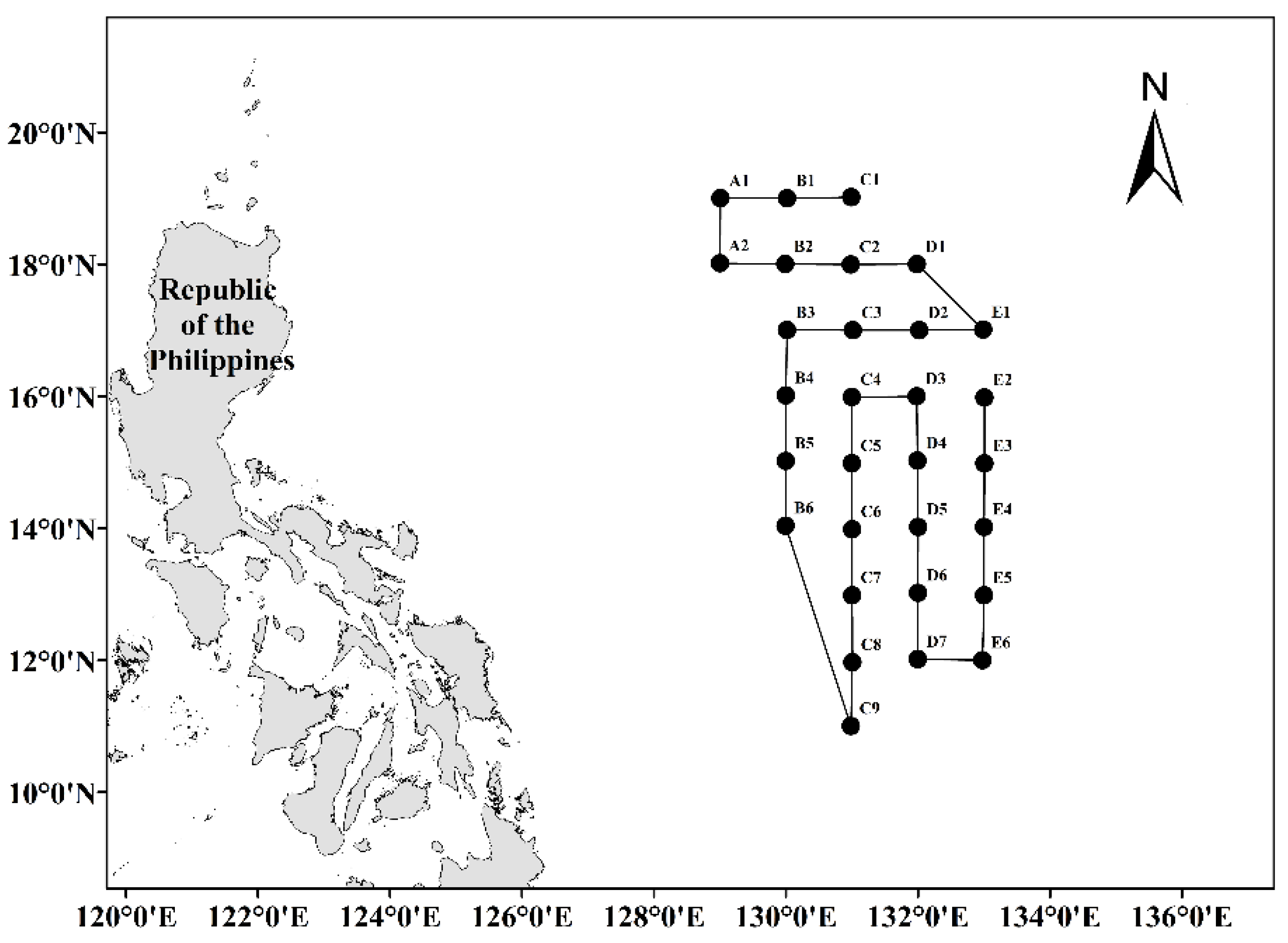
2.1. Survey Information

Acoustic and environmental data were collected onboard the research vessel (RV) Songhang. The vessel measures 85 m in length, 8.7 m in depth, and 3271.4 t in displacement when fully loaded. Using a fixed-point sampling method, the survey was conducted via a non-stop voyage from 15 August to 29 August 2022. A total of 30 stations were designed to collect environmental data during the survey, which took place in the NEC region of the Central and Western Pacific Ocean (11–19° N, 129–133° E). The geographic route and CTD profiling points of the survey are presented in Figure 1. Acoustic profiling occurred along the mapped trajectory (line), and CTD profiles were taken at point locations. A total of four trawls were set up during the survey for auxiliary acoustic calculations, and the trawl sampling stations were B2, D1, E1, and C3.

2.2. Data Collection

Simrad EK80 (Kongsberg Maritime AS, Horten, Norway) echo sounders are versatile instruments with various frequency transducers for simultaneous data acquisition capable of broadband detection. The echo sounders were calibrated in situ by standard techniques [32], following the calibration procedure outlined in the Simrad EK80 reference manual. The primary parameters of EK80 during the survey are detailed in Table 1. For this study, which focuses on shallow acoustic scattering, 38 kHz frequency transducers were exclusively utilized owing to their superior signal-to-noise ratio (SNR) and excellent data quality. Additionally, previous research has established that 38 kHz can detect zooplankton and micronekton [33,34].
Environmental data, such as vertical water temperature, salinity, oxygen content, and pH, were acquired by the shipboard Sea-Bird SBE 911 plus CTD (Sea-Bird Electronics, Inc., Washington, DC, USA). The CTD data (environmental factors) collection time for each station is about 30 min. The sampling time and date of each station are shown in Table 2.
The biological samples were collected by a four-piece mesopelagic trawl net with a single capsule structure, with overall dimensions of 434 m by 97.1 m (44.98 m). The machine-woven mesh was used for the net body, and the large mesh was used for the net port. A single-hand steel connection was used to connect two leaf mesh boards. The trawl design is well-suited for operations in variable water layers, ranging from 0 to 500 m in depth. Additionally, the net mouth of the trawl can expand horizontally and vertically by approximately 30 m. The average towing speed was 4.9 kn, and the average trawling time was 1.25 h.

2.3. Data Processing

The data collected in this survey were analyzed and processed using the acoustic data processing software Echoview 13.0, which applies a combination of built-in algorithms for data noise removal and integration processing. The echosounder calibration files were imported into Echoview to correct the original data. The software utilizes multiple variables, such as “background noise removal”, “impulse noise removal”, and “mask noise removal”, to remove background noise and random noise from the echograms [35,36,37]. The integration range is from 10 m below the transducer surface to a depth of 200 m. The basic integration voyage unit is set to 1 nautical mile in the horizontal direction and 50 m in the vertical direction. An integration threshold of −75 dB is set to mask weak scattered echo signals in the echogram. Based on the integration process of the software, the Sv and the NASC are obtained for each integration cell. To understand the distribution of biological resources in different water depths within the surveyed sea area, the NASC and Sv of each water layer throughout the entire integration voyage were homogenized. The same is done with acoustic data collected at various stations when the vessel is stopped. The mean value of Sv is derived using the following equation:
S v ¯ = 10 l o g 10 i = 1 n 10 S v i / 10 n
where S v i is the scattering strength of each water layer at nautical mile i, and n is the total number of nautical miles.

2.4. Solar Altitude Angle Acquisition

Due to the different times of data collection at each station during the survey and the other light intensity at the sea surface, to analyze the variation of DVM of SSL with the solar altitude angle (which represents the light intensity to some extent), this paper uses the solar angle calculator provided by the Earth System Research Lab (NOAA, Washington, DC, USA) to obtain the solar altitude angle according to the longitude and latitude position of each survey station and the corresponding UTC [38].

2.5. Generalized Additive Model

The GAM is a nonparametric extension of the generalized linear model introduced by Hastie and Tibshirani [39] in 1896, which intuitively models the nonlinear relationship between explanatory and response variables. In this study, the scattering layer’s Sv was higher than in other water layers. Thus, the scattering strength in the scattering layer was manually matched to the CTD environmental data based on the time–depth distribution of the Sv. The response variable of the GAM is the mean Sv at each station, representing the metric corresponding to the SSL. For the GAM, longitude and latitude were used as spatial factors. The solar altitude angle was deemed to be closely related to the DVM of biomass. Current velocity was found to have a direct effect on Sv. At the same time, temperature, salinity, dissolved oxygen, chlorophyll concentration, and seawater turbidity were identified as drivers of plankton’s spatial and temporal variation. Therefore, the predictor variables in the model include longitude, latitude, solar altitude angle, seawater density, temperature, seawater flow rate, salinity, dissolved oxygen, chlorophyll concentration, and seawater turbidity. The full factorial expression of the GAM is presented as follows:
S v ~ s L a t + s L o n + s S o l + s ρ + s T + s C v + s S + s D O + s C h l + s ( T u r ) + ε
The sample smoothing function s() (also known as smoothing spline) can be applied to univariate and multivariate smoothing of each sex, using Gaussian distribution. The variables used in the model include Lat for latitude (° N), Lon for longitude (° E), Sol for solar altitude angle (°), ρ for seawater density (kg/m³), T for temperature (°C), Cv for seawater flow rate (m/s), S for salinity (PSU), DO for dissolved oxygen (mg/L), Chl for chlorophyll concentration (μg/L), and Tur for seawater turbidity (NTU). The Sv data were preprocessed to construct the model. The covariance of predictor variables was evaluated using the variance inflation factor (VIF), with a critical value of 3 [40], and variables with VIF greater than 3 were removed. The GAM was established, and the stepwise regression and model prediction was performed using the mgcv package in R language software (V4.2.2).
V I F = 1 1 c o r 2
VIF refers to the variance inflation factor, and cor refers to the correlation coefficient between the elements, using Pearson’s correlation method [41]. For model testing, Akai’s Information Criterion (AIC) was used to test the fit of the model after adding the factors. Secondly, the p-value was used to test whether the elements were significant in the model [42].

3. Results and Analysis

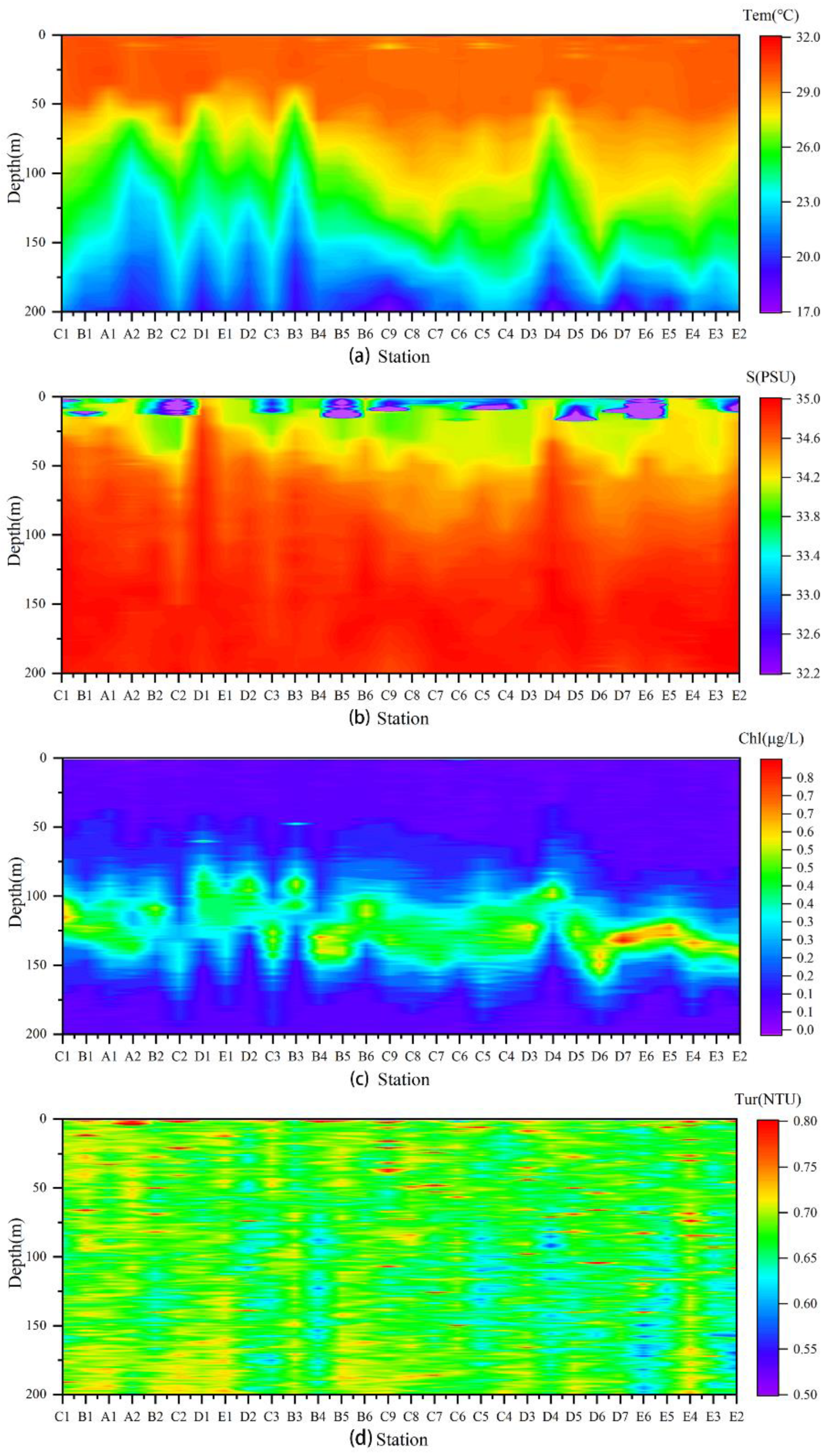
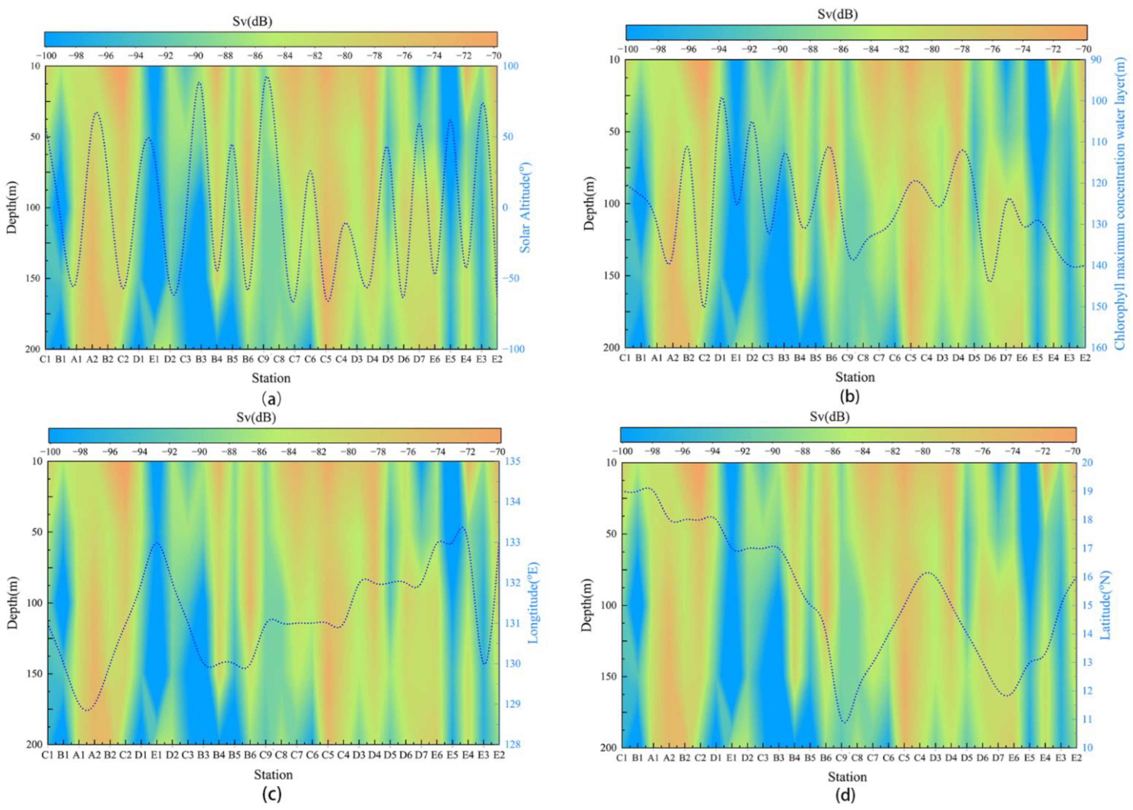
3.1. Vertical Distribution of Environmental Data at Each Station

The vertical distribution of environmental data at each station is shown in Figure 2; the temperature in Figure 2a gradually decreases with the increase in the seawater depth, and the lowest temperature is 17 °C at 200 m. Figure 2b shows the vertical distribution of the seawater salinity; the range of seawater salinity is 32.2–35 PSU. Figure 2c shows the vertical distribution of the chlorophyll concentration; the overall view of the maximum chlorophyll concentration water layer is located at 100–150 m. Figure 2d shows the vertical distribution of the seawater turbidity; the range of seawater turbidity is 0.5–0.8 NTU.

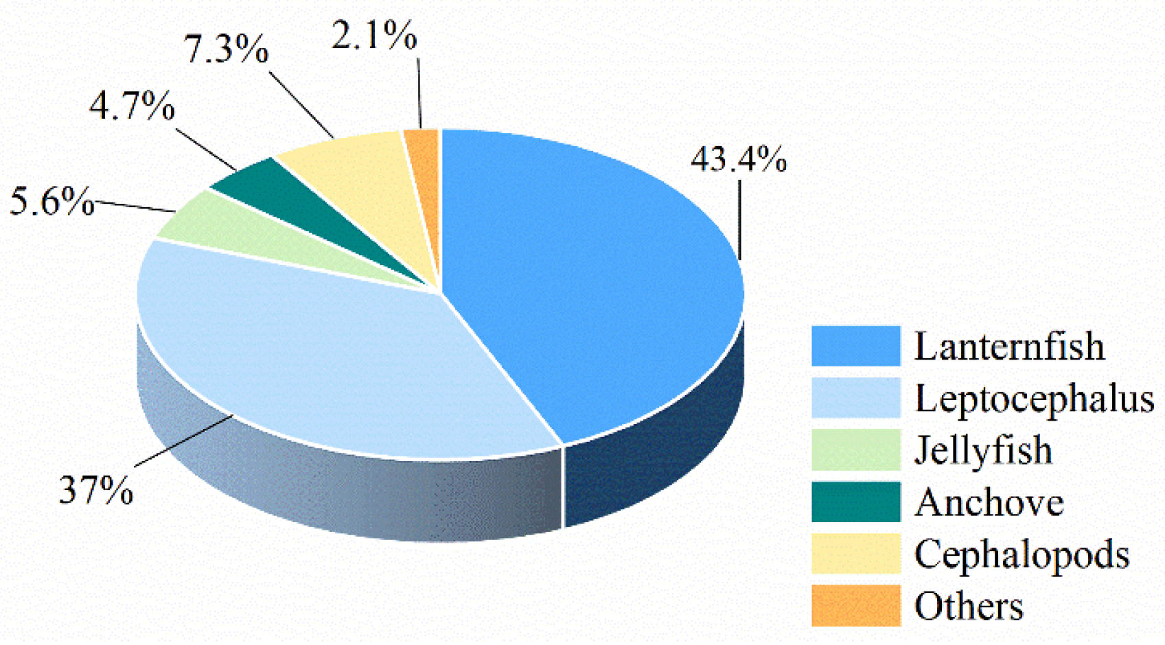
3.2. Information about the Catch

Four trawl surveys were conducted during this cruise, and the main catches were micronekton and zooplankton, including Lanternfish, leptocephalus, jellyfish, etc. The body length of Lanternfish ranges from 27 mm to 36 mm, with an average of 32.56 mm. The body length of leptocephalus ranges from 73 mm to 285 mm, with an average of 209.65 mm. The body length of Jellyfish ranges from 25 mm to 46 mm, with an average of 36.18 mm. The body length of Anchove ranges from 37 mm to 54 mm, with an average of 46.4 mm. The mantle length of Cephalopods ranges from 25 mm to 136 mm, with an average of is 95.35 mm. The proportion of each species in the catches is shown in Figure 3. The highest proportion of Lanternfish was 43.4%, followed by leptocephalus with 37.6%, which indicates that the primary scatterers in the warm pool area of the North Equatorial Current in the Central and Western Pacific Ocean are micronekton and zooplankton.

3.3. General Characteristics of Sound Scattering

The volume-backscatter strength values in the shallow water layer at 200 m mainly ranged from −100 dB to −70 dB. Judging from the echogram, the scattering layer echo strength also falls within this range. To accurately invert the distribution pattern of the scattering layer using the echo intensity data of the water body measured by EK80 and to visually observe the SSL distribution, the scattering map only displays the range of −100 dB to −70 dB (as shown in Figure 4). Overall, the Sv of different water layers differed considerably. The scattering strength was more pronounced in the 10–50 m water layer than in other water layers and gradually decreased with the increase in water depth. The surveyed sea area has an obvious SSL distributed in the shallow water layer of 10–90 m.

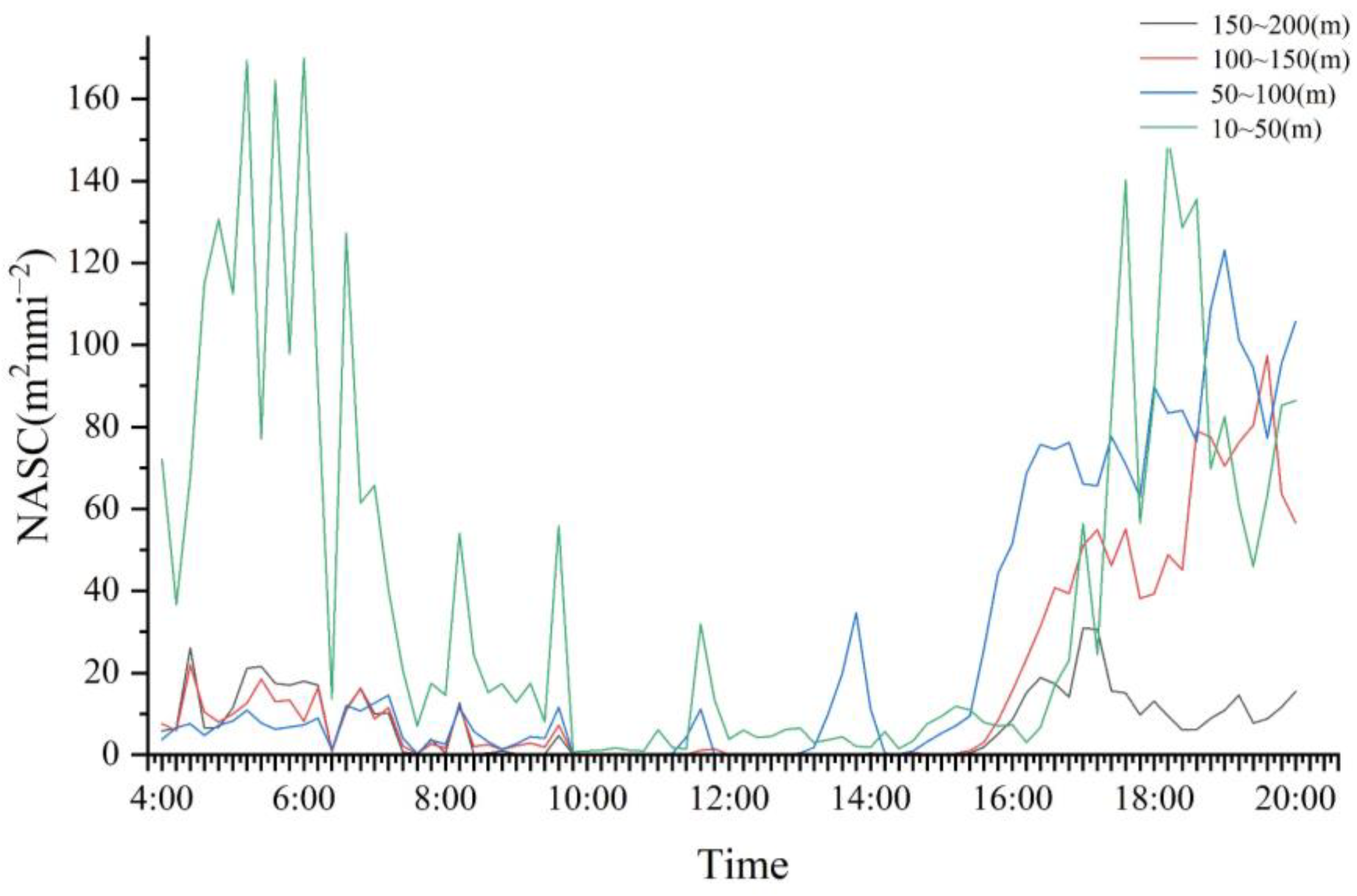
3.4. Vertical Distribution of Average Sv in Different Water Layers

Figure 5 shows the continuous changes in NASC values in different water layers on 25th August. The NASC value decreased significantly between 6:00 and 7:00, indicating that SSL migrated from the surface to deeper waters. The NASC value increased significantly between 17:00 and 18:00, indicating that SSL migrated from deeper waters to the surface. The NASC values in all water layers reached their lowest point at noon (12:00). The diurnal variation trend in SSL confirms the DVM phenomenon. Overall, the scatters mainly concentrated within the 10–50 m water layer and gradually decreased with an increase in water depth.

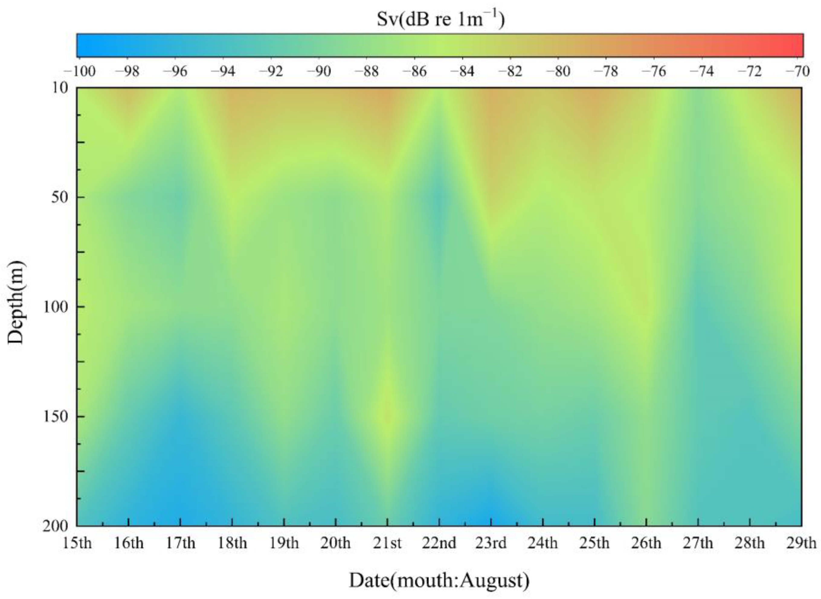
3.5. Diel Variation of Scattering Strength

Figure 6 compares each station’s Sv and the solar altitude angle at different water layers. The solar altitude angle was positive during the day and negative at night. The results indicate that Sv was relatively low at stations C1, E1, B3, B5, C9, D5, E5, and E3. The Sv varied significantly among stations, mainly manifested in different depths of the high scattering values, such as stations A2, B2, C5, and D7, where the high scattering values extend deeper. The scattering strength gradually decreased within the same station with increasing water depth. Overall, the variation trend of the Sv at each station showed strong temporal synchronicity with the solar altitude angle. Compared with daytime, the Sv was higher at night, indicating a DVM of the scattering layer. No significant correlation was observed between the Sv and the maximum chlorophyll concentration layer. No clear pattern of change was observed, indicating that the Sv is unaffected by chlorophyll concentration. The longitude range during the cruise was between 129 and 133° E. The Sv gradually decreased with increasing longitude from stations A2 to D4, while no significant changes were observed from stations E1 to D3 with decreasing longitude. The latitude range during the cruise was between 11 and 19° N. The Sv increased with increasing latitude from stations C9 to D4 and gradually decreased with a decreasing margin from stations D3 to D7, indicating that Sv is affected by longitude and latitude.

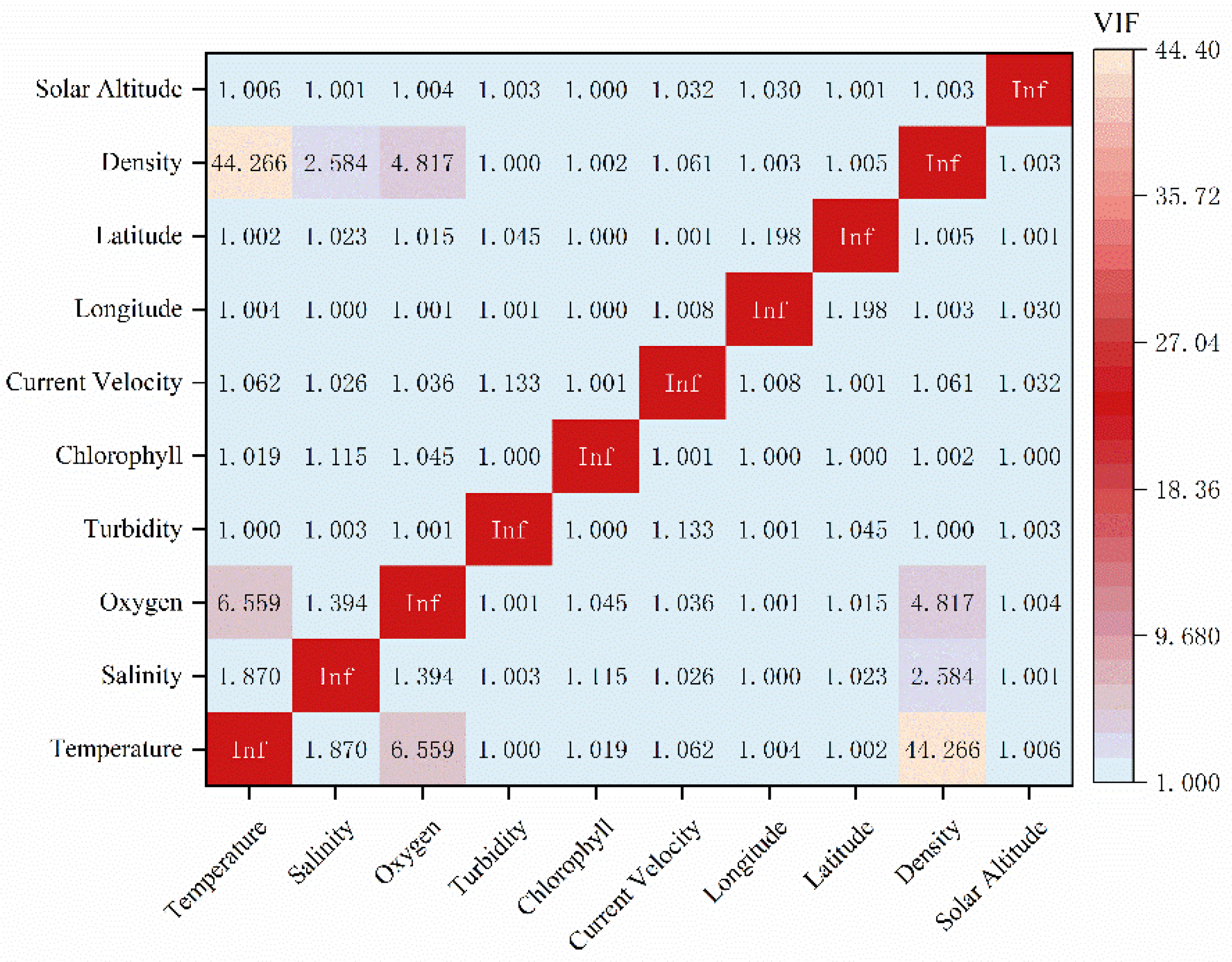
3.6. Covariance Test of Predictor Variables

Among the ten predictor variables, the VIF values of temperature, density, and oxygen content were all greater than 3. The VIF values of the remaining seven variables, such as latitude and longitude, were all less than 3 (Figure 7). Since temperature is an essential factor affecting the scattering layer distribution [43], density and oxygen content were removed. After removing the variables with VIF more significant than 3, the VIF values of the remaining eight predictor variables were less than 3. Therefore, eight predictor variables, including longitude, latitude, solar altitude angle, temperature, turbidity, chlorophyll concentration, salinity, and current velocity, were used for the GAM building.

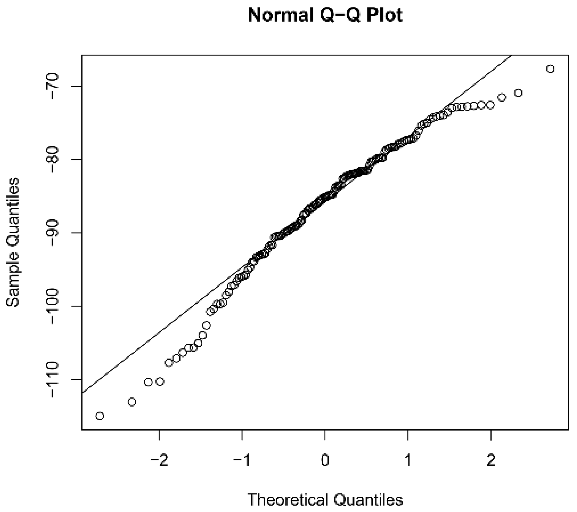
3.7. Factorial Significance Test

Table 3 shows the sequence of the study object and factor, which can prove the fitting rationality of the model and the importance of the next research factor. The AIC was used to test the model’s fit after adding the explanatory variables, and a smaller value of AIC indicates a better fit of the model [44]. The AIC was not significantly reduced when salinity and chlorophyll factors were included, so they were excluded from this study. The final optimized model was:
S v ~ s T + s T u r + s S o l + s C V + s L a t + s L o n + ε

3.8. GAM Test Results

The GAM test results showed that the total bias explanation rate was 67.2% (Table 4). Among the factors used to construct the model, the solar altitude angle had the most significant effect on the scattering strength with the highest bias explanation rate of 35.4%, followed by latitude (12.7%), longitude (8.2%), temperature (5.05%), turbidity (5.05%), and current velocity (0.8%). The results of the GAM test and the residual distribution plots indicate that the final chosen model can better explain the influencing factors of the acoustic scattering layer distribution (Figure 8).

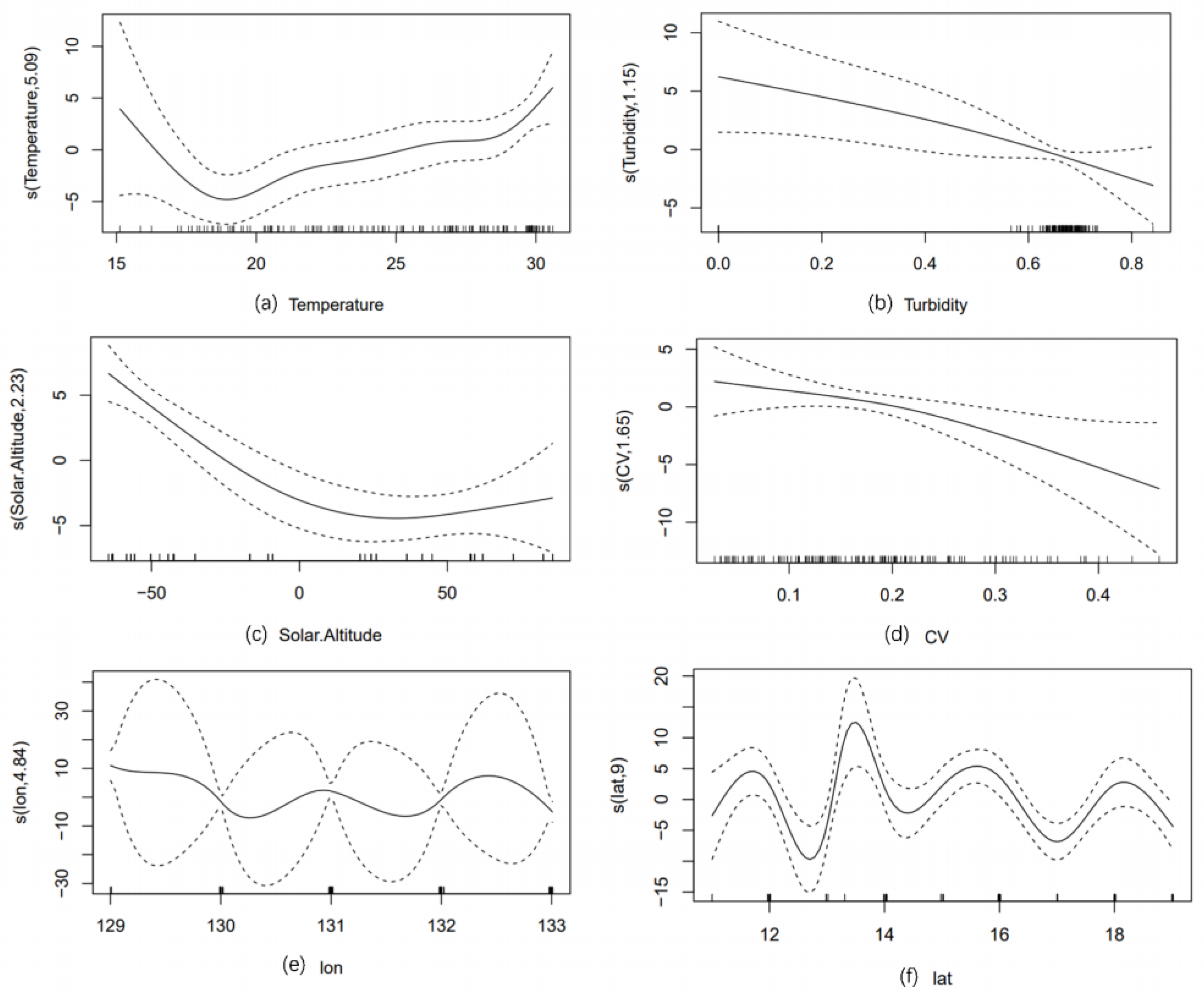
3.9. Relationship between Scattering Strength and Environmental Factors

Within the range of 15 °C to 30 °C, a nonlinear relationship could be observed between temperature and scattering strength, with a decrease followed by an increase. The minimum scattering strength was observed at 18 °C (Figure 9a). Within the range of 0.5 NTU to 0.75 NTU, a negative nonlinear relationship could be observed between turbidity and scattering strength (Figure 9b). Within the −90° to 90° range, a negative nonlinear relationship exists between solar altitude angle and scattering strength (Figure 9c). Within the scope of 0 m/s to 0.5 m/s, there was a negative nonlinear relationship between current sea velocity and scattering strength (Figure 9d). Within the range of 129° E to 133° E, a nonlinear relationship could be seen between longitude and scattering strength, with a decreasing trend followed by an increasing trend and then another decreasing trend as longitude increases (Figure 9e). Within the range of 11° N to 19° N, there was a nonlinear relationship with multiple peaks between latitude and scattering strength (Figure 9f).

4. Discussion

The laterally continuous SSL is often widely distributed in oceans. Because the Sv values in this survey were mostly between −100 dB and −70 dB, non-biological backscattering in the sea had little effect on the observed SSL [45]. According to Batzler [46] and others, the scattering strength values of the zooplankton scattering layer range from −95 dB to −50 dB, which is consistent with the overall sound-scattering characteristics in this survey and conforms to the scattering parts of the zooplankton layer. Combined with the trawl survey results, the main scatterers in the shallow scattering layer of the sea were judged to be zooplankton and micronekton. The SSL is distributed in water depths of 100 m or less in the horizontal direction, with an average thickness of 50 m (Figure 4), consistent with Li et al.’s research results [47].
The NASC is a valuable index for indicating the distribution of plankton and fish [48]. Figure 5 shows significant differences in NASC values among different water layers, with plankton and micronekton mostly aggregating in water shallower than 100 m, and the biological distribution becoming scarcer as the water depth increases. Figure 5 shows SSL exhibits DVM, with the biomass significantly decreasing during the daytime and increasing at night. The variation in NASC values generally follows the DVM pattern of the scattering layer. The DVM of the scattering layer is a behavioral mechanism typically characterized by plankton and micronekton ascending to feed at night and descending to deeper layers during the day to avoid higher trophic-level predators [7]. Biological factors and abiotic factors, such as light intensity, water transparency, and water temperature, influence the DVM of the scattering layer. For example, when a solar eclipse occurs at noon, the light intensity sharply decreases, accompanied by the vertical migration of the scattering layer. This suggests that the DVM of the scattering layer is primarily controlled by light [49]. Therefore, we need to consider multiple environmental factors to comprehensively understand and predict the occurrence and ecological significance of the DVM of the scattering layer.
The DVM phenomenon of the scattering layer is widely present in the ocean. Studying the marine scattering layer is beneficial to understanding the marine ecosystem. The main environmental elements in the current international research progress on the scattering layer include temperature, oxygen content, light intensity, latitude, and longitude [50], among which light is considered the most crucial cause of DVM behavior [51]. In this study, the GAM consists of several factors: longitude, latitude, temperature, turbidity, solar altitude angle, and current velocity. The greater the solar altitude angle, the shorter the path through the atmosphere, the less the weakening effect of the atmosphere on solar radiation, and the stronger the solar radiation reaching the sea surface. According to the field investigation records, the weather conditions during the sampling period at stations A2 and D7 were cloudy, and the rest of the stations were sunny. Taking into account the attenuation of light intensity in seawater, we analyzed the relationship between the solar altitude angle and the scattering strength in the water column at each station. Figure 6a shows the solar height angle. The change of the altitude angle has a more significant impact on the scattering strength in the water column, and the changing trend between the two has a strong time–series correlation, so to some extent, we can use the solar altitude angle as a reference indicator of the light intensity at the sea surface to analyze the relationship between light and scattering strength. Among the performance results of the GAM, the solar altitude angle predicted that the scattering strength is significant, with the highest contribution of 35.4%, indicating that light intensity is the most dominant environmental factor affecting the diurnal migration of the scattering layer, which is consistent with the findings of Boswell et al. [27] and further corroborates the relative accuracy of the GAM results. The phenomenon of light affecting DVM in the scattering layer suggests that zooplankton are light-avoidant, mainly by zooplankton and micronekton, to reduce the risk of predation [11]. There was no significant pattern between scattering strength and chlorophyll concentration, as seen in Figure 6b. Chlorophyll concentration is similarly insignificant in the GAM, so the distribution of the scattering layer is not affected by chlorophyll concentration, consistent with the conclusion that the DVM behavior of the scattering layer is independent of chlorophyll reached by Rosalie et al. [52]. The Sv in Figure 9b decreases with the increasing turbidity of the seawater, which may be caused by the fact that increasing turbidity reduces the detection distance and recognition ability of visual predators, thus leading to a decrease in scattering strength. This agrees with the findings of Graeme et al. [53]. Among the spatial and temporal variables, latitude and longitude have a significant effect on the prediction of scattering strength, with a high contribution rate of 20.9%, showing a strong correlation, indicating that the scattering strength is influenced by latitude and longitude, but because the data of latitude and longitude corresponding to each station are small, the latitude and longitude are mainly concentrated in integers; the factor effect relationship diagram must accurately reflect the changing pattern of scattering strength, latitude, and longitude. The accumulation of data volume should be increased in the later stage, and the collection of data later expanded.
The NEC warm pool is a typical tropical marine ecosystem with a large warm surface current flowing northward. The wind, which originates in the equatorial region, is heated by intense solar radiation, resulting in a relatively high water temperature and a fast flow rate averaging around 70 cm/s and occasionally reaching 200 cm/s [54]. The temperature and flow velocity of the NEC has essential effects on the migration of SSL. As a result, the NEC’s flow velocity and temperature can influence the distribution and migration of SSL in the ocean. The flow velocity and scattering strength have a negative nonlinear connection in the factor effect diagram (Figure 9d), which is consistent with the results of Li et al. [47]. Yang et al. [55] discovered that during typhoons, the flow velocity increased and the DVM of SSL creatures deteriorated, which is consistent with the conclusion drawn in our investigation that the scattering strength decreased with increasing flow velocity. The significant environmental characteristic of the study area is continual high temperature, which was also an essential factor affecting the distribution of planktonic organisms in the GAM, with a contribution rate of 5.05%. Temperature is significantly correlated with the scattering strength (p ≤ 0.001). The temperature range of the NEC warm pool is 15–30 °C, with a large confidence interval and low credibility at 15–18 °C and a nonlinear positive correlation between temperature and scattering strength at 18–30 °C, indicating that planktonic organisms and micronekton tend to live in warmer areas, consistent with previous research results [56]. Therefore, it is speculated that high temperature provides a favorable environment for the growth and reproduction of SSL, shortening the generation time and increasing their reproductive rate and biomass under high-temperature conditions.

5. Conclusions

This study investigated the characteristics of SSL and their relationships with environmental factors in the NEC region of the Central and Western Pacific Ocean. By combining acoustic indices with the GAM, we analyzed the influence of multiple environmental factors on scattering strength from the perspective of the living environment of zooplankton and micronekton. The main finding of this study is the presence of a continuous and persistent scattering layer in the surface layer of the research area, and the primary scatterers are zooplankton and micronekton, which exhibit diel vertical migration. Light intensity is the most important environmental factor affecting the DVM of the scattering layers. These results provide a reference for the long-term study of environmental changes and their effects on the distribution of micronekton and zooplankton communities and enrich the relevant research on SSL in the Central and Western Pacific Ocean. In future research, it is necessary to comprehensively consider more environmental factors in order to better understand and predict the occurrence and ecological significance of diel vertical migration of scattering layers.

Author Contributions

Methodology, J.T. and M.X.; formal analysis, T.G. and Z.Z.; environmental data analysis, J.L.; software, T.G. and Y.Q.; writing—original draft preparation, T.G. and J.T.; writing—review and editing, J.T., R.K. and Q.M. All authors have read and agreed to the published version of the manuscript.

Funding

This research was funded by the National Key R&D Program of China (2019YFD0901401), the Key Laboratory of Marine Ecological Monitoring and Restoration Technologies (MEMRT202202), and the National Natural Science Foundation of China (32202934). We also acknowledge funds provided by the Ministry of Agriculture and Rural Affairs of China, through the project on the Survey and Monitor-Evaluation of Global Fishery Resources.

Institutional Review Board Statement

Not applicable.

Informed Consent Statement

Not applicable.

Data Availability Statement

The authors declare that the data supporting the findings of this study are available within the article or are available from the corresponding authors upon request.

Acknowledgments

The authors of this research would like to thank all the researchers and sailors on RV Songhang.

Conflicts of Interest

The authors declare no conflict of interest.

References

  1. Guo, J.R.; Liu, Y.L.; Song, J.; Bao, X.W.; Li, Y.; Chen, S.Y.; Yang, J.K. The west boundary bifurcation line of the North Equatorial Current in the Pacific changes features. J. Ocean Univ. China 2015, 14, 957–968. [Google Scholar] [CrossRef]
  2. Tan, S.W.; Zhou, H. The observed impacts of the two types of El Niño on the North Equatorial Countercurrent in the Pacific Ocean. Geophys. Res. Lett. 2018, 45, 493–500. [Google Scholar] [CrossRef] [Green Version]
  3. Chen, H.; Shi, J.; Jin, Y.S.; Geng, T.; Li, C.; Zhang, X.Z. Warm and cold episodes in western Pacific warm pool and their linkage with ENSO asymmetry and diversity. J. Geophys. Res. Oceans 2021, 126, e2021J–e17287J. [Google Scholar] [CrossRef]
  4. Lin, M.; Wang, C.G.; Wang, Y.G.; Xiang, P.; Wang, Y.; Lian, G.S.; Chen, R.X.; Chen, X.Y.; Ye, Y.Y.; Dai, Y.Y. Zooplanktonic diversity in the western Pacific. Biodivers. Sci. 2011, 19, 646–654. [Google Scholar]
  5. Davison, P.C.; Checkley, D.M., Jr.; Koslow, J.A.; Barlow, J. Carbon export mediated by mesopelagic fishes in the northeast Pacific Ocean. Prog. Oceanogr. 2013, 116, 14–30. [Google Scholar] [CrossRef]
  6. Hylander, S.; Larsson, N.; Hansson, L. Zooplankton vertical migration and plasticity of pigmentation arising from simultaneous UV and predation threats. Limnol. Oceanogr. 2009, 54, 483–491. [Google Scholar] [CrossRef]
  7. Kang, M.; Kang, J.; Kim, M.; Nam, S.; Choi, Y.; Kang, D. Sound Scattering Layers Within and Beyond the Seychelles-Chagos Thermocline Ridge in the Southwest Indian Ocean. Front. Mar. Sci. 2021, 8, 769414. [Google Scholar] [CrossRef]
  8. Takahashi, K.; Kuwata, A.; Sugisaki, H.; Uchikawa, K.; Saito, H. Downward carbon transport by diel vertical migration of the copepods Metridia pacifica and Metridia okhotensis in the Oyashio region of the western subarctic Pacific Ocean. Deep Sea Res. Part I Oceanogr. Res. Pap. 2009, 56, 1777–1791. [Google Scholar] [CrossRef]
  9. Ducklow, H.W.; Steinberg, D.K.; Buesseler, K.O. Upper ocean carbon export and the biological pump. Oceanography 2001, 14, 50–58. [Google Scholar] [CrossRef]
  10. Proud, R.; Cox, M.J.; Le Guen, C.; Brierley, A.S. Fine-scale depth structure of pelagic communities throughout the global ocean based on acoustic sound scattering layers. Mar. Ecol. Prog. Ser. 2018, 598, 35–48. [Google Scholar] [CrossRef] [Green Version]
  11. Bianchi, D.; Stock, C.; Galbraith, E.D.; Sarmiento, J.L. Diel vertical migration: Ecological controls and impacts on the biological pump in a one-dimensional ocean model. Global Biogeochem. Cycles 2013, 27, 478–491. [Google Scholar] [CrossRef]
  12. Priou, P.; Nikolopoulos, A.; Flores, H.; Gradinger, R.; Kunisch, E.; Katlein, C.; Castellani, G.; Linders, T.; Berge, J.; Fisher, J.A. Dense mesopelagic sound scattering layer and vertical segregation of pelagic organisms at the Arctic-Atlantic gateway during the midnight sun. Prog. Oceanogr. 2021, 196, 102611. [Google Scholar] [CrossRef]
  13. Norheim, E.; Klevjer, T.A.; Aksnes, D.L. Evidence for light-controlled migration amplitude of a sound scattering layer in the Norwegian Sea. Mar. Ecol. Prog. Ser. 2016, 551, 45–52. [Google Scholar] [CrossRef] [Green Version]
  14. Flagg, C.N.; Smith, S.L. On the use of the acoustic Doppler current profiler to measure zooplankton abundance. Deep Sea Res. Part I Oceanogr. Res. Pap. 1989, 36, 455–474. [Google Scholar] [CrossRef]
  15. Ashjian, C.J.; Smith, S.L.; Flagg, C.N.; Mariano, A.J.; Behrens, W.J.; Lane, P.V. The influence of a Gulf Stream meander on the distribution of zooplankton biomass in the Slope Water, the Gulf Stream, and the Sargasso Sea, described using a shipboard acoustic Doppler current profiler. Deep Sea Res. Part I Oceanogr. Res. Pap. 1994, 41, 23–50. [Google Scholar] [CrossRef]
  16. Wishner, K.F.; Seibel, B.A.; Roman, C.; Deutsch, C.; Outram, D.; Shaw, C.T.; Birk, M.A.; Mislan, K.; Adams, T.J.; Moore, D. Ocean deoxygenation and zooplankton: Very small oxygen differences matter. Sci. Adv. 2018, 4, u5180. [Google Scholar] [CrossRef] [Green Version]
  17. Xu, Y.J.; Zhao, L.; Yuan, Y. The diel vertical migration of zooplankton observed by an acoustic Doppler current profiler and particle size analyzer in the East China Sea. Acta Oceanol. Sin. 2016, 38, 124–131. [Google Scholar]
  18. Sourisseau, M.; Simard, Y.; Saucier, F.J. Krill diel vertical migration fine dynamics, nocturnal overturns, and their roles for aggregation in stratified flows. Can. J. Fish. Aquat. Sci. 2008, 65, 574–587. [Google Scholar] [CrossRef]
  19. Whitmore, B.M.; Nickels, C.F.; Ohman, M.D. A comparison between Zooglider and shipboard net and acoustic mesozooplankton sensing systems. J. Plankton Res. 2019, 41, 521–533. [Google Scholar] [CrossRef]
  20. Murase, H.; Nagashima, H.; Yonezaki, S.; Matsukura, R.; Kitakado, T. Application of a generalized additive model (GAM) to reveal relationships between environmental factors and distributions of pelagic fish and krill: A case study in Sendai Bay, Japan. ICES J. Mar. Sci. 2009, 66, 1417–1424. [Google Scholar] [CrossRef] [Green Version]
  21. Kim, J.Y.; Lee, J.B.; Suh, Y. Oceanographic indicators for the occurrence of anchovy eggs inferred from generalized additive models. Fish. Aquat. Sci. 2020, 23, 19. [Google Scholar] [CrossRef]
  22. Bigelow, K.A.; Boggs, C.H.; He, X.I. Environmental effects on swordfish and blue shark catch rates in the US North Pacific longline fishery. Fish. Oceanogr. 1999, 8, 178–198. [Google Scholar] [CrossRef]
  23. Yalçın, E.; Gurbet, R. Environmental Influences on the Spatio-Temporal Distribution of European Hake (Merluccius merluccius) in Izmir Bay, Aegean Sea. Turk. J. Fish. Aquat. Sci. 2016, 16, 1–14. [Google Scholar] [CrossRef]
  24. Feng, Y.T.; Shi, H.Y.; Hou, G.; Zhao, H.; Dong, C.M. Relationships between environmental variables and spatial and temporal distribution of jack mackerel (Trachurus japonicus) in the Beibu Gulf, South China Sea. PeerJ 2021, 9, e12337. [Google Scholar] [CrossRef] [PubMed]
  25. Khan, A.M.; Nasution, A.M.; Purba, N.P.; Rizal, A.; Hamdani, H.; Dewanti, L.P.; Nurruhwati, I.; Sahidin, A.; Supriyadi, D.; Herawati, H. Oceanographic characteristics at fish aggregating device sites for tuna pole-and-line fishery in eastern Indonesia. Fish. Res. 2020, 225, 105471. [Google Scholar] [CrossRef]
  26. Hughes, K.M.; Dransfeld, L.; Johnson, M.P. Climate and stock influences the spread and locations of catches in the northeast Atlantic mackerel fishery. Fish. Oceanogr. 2015, 24, 540–552. [Google Scholar] [CrossRef]
  27. Boswell, K.M.; D’Elia, M.; Johnston, M.W.; Mohan, J.A.; Warren, J.D.; Wells, R.D.; Sutton, T.T. Oceanographic structure and light levels drive patterns of sound scattering layers in a low-latitude oceanic system. Front. Mar. Sci. 2020, 7, 51. [Google Scholar] [CrossRef]
  28. Lee, H.; La, H.S.; Kang, D.; Lee, S. Vertical distribution of the sound-scattering layer in the Amundsen Sea, Antarctica. Polar Sci. 2018, 15, 55–61. [Google Scholar] [CrossRef]
  29. Yin, X.Q.; Yang, D.T.; Zhao, L.H.; Zhong, R.; Du, R.R. Fishery Resource Evaluation with Hydroacoustic and Remote Sensing in Yangjiang Coastal Waters in Summer. Remote Sens. 2023, 15, 543. [Google Scholar] [CrossRef]
  30. Darnis, G.; Hobbs, L.; Geoffroy, M.; Grenvald, J.C.; Renaud, P.E.; Berge, J.; Cottier, F.; Kristiansen, S.; Daase, M.; Søreide, J.E. From polar night to midnight sun: Diel vertical migration, metabolism and biogeochemical role of zooplankton in a high Arctic fjord (Kongsfjorden, Svalbard). Limnol. Oceanogr. 2017, 62, 1586–1605. [Google Scholar] [CrossRef] [Green Version]
  31. Burd, A.C.; Lee, A.J. The sonic scattering layer in the sea. Nature 1951, 167, 624–626. [Google Scholar] [CrossRef]
  32. Demer, D.; Berger, L.; Bernasconi, M.; Bethke, E.; Boswell, K.; Chu, D.; Domokos, R.; Dunford, A.; Fassler, S.; Gauthier, S. Calibration of acoustic instruments. ICES Coop. Res. Rep. 2015, 326, 133pp. [Google Scholar]
  33. Mouget, A.; Brehmer, P.; Perrot, Y.; Uanivi, U.; Diogoul, N.; El Ayoubi, S.; Jeyid, M.A.; Sarré, A.; Béhagle, N.; Kouassi, A.M. Applying acoustic scattering layer descriptors to depict mid-trophic pelagic organisation: The case of Atlantic African large marine ecosystems continental shelf. Fishes 2022, 7, 86. [Google Scholar] [CrossRef]
  34. Ariza, A.; Landeira, J.M.; Escánez, A.; Wienerroither, R.; de Soto, N.A.; Røstad, A.; Kaartvedt, S.; Hernández-León, S. Vertical distribution, composition and migratory patterns of acoustic scattering layers in the Canary Islands. J. Mar. Syst. 2016, 157, 82–91. [Google Scholar] [CrossRef] [Green Version]
  35. Wang, X.; Zhang, J.; Zhao, X. A post-processing method to remove interference noise from acoustic data collected from Antarctic krill fishing vessels. CCAMLR Sci. 2016, 23, 17–30. [Google Scholar]
  36. Korneliussen, R.J. Measurement and removal of echo integration noise. ICES J. Mar. Sci. 2000, 57, 1204–1217. [Google Scholar] [CrossRef] [Green Version]
  37. Watkins, J.L.; Brierley, A.S. A post-processing technique to remove background noise from echo integration data. ICES J. Mar. Sci. 1996, 53, 339–344. [Google Scholar] [CrossRef] [Green Version]
  38. Solar Calculations: Solar Calculator. Available online: https://gml.noaa.gov/grad/solcalc (accessed on 20 February 2023).
  39. Hastie, T.; Tibshirani, R. Generalized Additive Models. Stat. Sci. 1986, 1, 297–318. [Google Scholar] [CrossRef]
  40. Han, H.B.; Yang, C.; Zhang, H.; Fang, Z.; Jiang, B.H.; Su, B.; Sui, J.H.; Yan, Y.Z.; Xiang, D.L. Environment variables affect CPUE and spatial distribution of fishing grounds on the light falling gear fishery in the Northwest Indian Ocean at different time scales. Front. Mar. Sci. 2022, 9, 939334. [Google Scholar] [CrossRef]
  41. Meng, W.Z.; Gong, Y.H.; Wang, X.F.; Tong, J.F.; Han, D.Y.; Chen, J.H.; Wu, J.H. Influence of spatial scale selection of environmental factors on the prediction of distribution of Coilia nasus in Changjiang River Estuary. Fishes 2021, 6, 48. [Google Scholar] [CrossRef]
  42. Syah, A.F.; Saitoh, S.; Alabia, I.D.; Hirawake, T. Detection of potential fishing zone for Pacific saury (Cololabis saira) using generalized additive model and remotely sensed data. In Proceedings of the IOP Conference Series: Earth and Environmental Science, Zvenigorod, Russia, 4–7 September 2017. [Google Scholar]
  43. Lee, H.; Cho, S.; Kim, W.; Kang, D. The diel vertical migration of the sound-scattering layer in the Yellow Sea Bottom Cold Water of the southeastern Yellow sea: Focus on its relationship with a temperature structure. Acta Oceanol. Sin. 2013, 32, 44–49. [Google Scholar] [CrossRef]
  44. Brodziak, J.; Walsh, W.A. Model selection and multimodel inference for standardizing catch rates of bycatch species: A case study of oceanic whitetip shark in the Hawaii-based longline fishery. Can. J. Fish. Aquat. Sci. 2013, 70, 1723–1740. [Google Scholar] [CrossRef]
  45. Urickr, J. Principles of Underwater Sound, 2nd ed.; McGraw-Hill Book: New York, NY, USA, 1975. [Google Scholar]
  46. Batzler, W.E.; Vent, R.J. Volume-Scattering Measurements at 12 kc/sec in the Western Pacific. J. Acoust. Soc. Am. 1967, 41, 154–157. [Google Scholar] [CrossRef]
  47. Li, Q.; Chen, Z.H. Diel Vertial migration of zooplankton in the Kuroshio-Oyashio Mixed Zone based on ADCP echo. Oceanol. Limnol. 2022, 2, 305–319. [Google Scholar]
  48. Costa, P.L.; Valderrama, P.R.C.; Madureira, L.A.S.P. Relationships between environmental features, distribution and abundance of the Argentine anchovy, Engraulis anchoita, on the South West Atlantic Continental Shelf. Fish. Res. 2016, 173, 229–235. [Google Scholar] [CrossRef]
  49. Franceschini, G.A.; Bright, T.J.; Caruthers, J.W.; El-Sayed, S.Z.; Vastano, A.C. Effects on migration of marine organisms in the Gulf of Mexico. Nature 1970, 226, 1155–1156. [Google Scholar] [CrossRef]
  50. Wiafe, G.; Yaqub, H.B.; Mensah, M.A.; Frid, C.L. Impact of climate change on long-term zooplankton biomass in the upwelling region of the Gulf of Guinea. ICES J. Mar. Sci. 2008, 65, 318–324. [Google Scholar] [CrossRef] [Green Version]
  51. Aksnes, D.L.; Røstad, A.; Kaartvedt, S.; Martinez, U.; Duarte, C.M.; Irigoien, X. Light penetration structures the deep acoustic scattering layers in the global ocean. Sci. Adv. 2017, 3, e1602468. [Google Scholar] [CrossRef] [Green Version]
  52. Evans, R.A.; Hopkins, C. Distribution and standing stock of zooplankton sound-scattering layers along the north Norwegian coast in February—March, 1978. Sarsia 1981, 66, 147–160. [Google Scholar] [CrossRef]
  53. Hays, G.C. A review of the adaptive significance and ecosystem consequences of zooplankton diel vertical migrations. Hydrobiologia 2003, 503, 163–170. [Google Scholar] [CrossRef]
  54. Hu, S.J.; Hu, D.X. Variability of the Pacific North Equatorial Current from repeated shipboard acoustic Doppler current profiler measurements. J. Oceanogr. 2014, 70, 559–571. [Google Scholar] [CrossRef]
  55. Ge, R.P.; Chen, H.J.; Liu, G.X.; Zhu, Y.Z.; Jiang, Q. Diel vertical migration of mesozooplankton in the northern Yellow Sea. J. Oceanol. Limnol. 2021, 39, 1373–1386. [Google Scholar] [CrossRef]
  56. Xue, M.H.; Tong, J.F.; Tian, S.Q.; Wang, X.F. Broadband Characteristics of Zooplankton Sound Scattering Layer in the Kuroshio–Oyashio Confluence Region of the Northwest Pacific Ocean in Summer of 2019. J. Mar. Sci. Eng. 2021, 9, 938. [Google Scholar] [CrossRef]
Figure 1. The distribution of 30 CTD stations during the 2022 Songhang survey in the Central and Western Pacific Ocean.
Jmse 11 01477 g001
Figure 2. Vertical distribution of environmental data at each station: (a) for temperature, (b) for salinity, (c) for chlorophyll concentration, and (d) for seawater turbidity.
Jmse 11 01477 g002
Figure 3. Proportion of each species in the catch.
Jmse 11 01477 g003
Figure 4. Distribution of the mean Sv across the entire voyage.
Jmse 11 01477 g004
Figure 5. The NASC trend in different water layers over time on August 25.
Jmse 11 01477 g005
Figure 6. Comparison of Sv values at each station with solar height angle (a), water layer with maximum chlorophyll concentration (b), longitude (c) and latitude (d) at the time of investigation. The dotted blue line represents the changing trend of environmental factors at each station.
Jmse 11 01477 g006
Figure 7. Results of collinearity test for predictor variables.
Jmse 11 01477 g007
Figure 8. Residual plot of the GAM for scattering strength.
Jmse 11 01477 g008
Figure 9. Influence of each factor on scattering strength in the GAM. The solid line represents the variation of the Sv with environmental factors. The dotted line represents the 95% confidence interval.
Jmse 11 01477 g009
Table 1. Main parameter settings of SIMRAD EK80.
Transducer TypeES38–7C
Beam typeSplitting
Broadband range/kHz34~45
Transmit power/W2000
Pulse length/ms1.024
Pulse interval/ms2000
Beam angle/°7
Table 2. Date and start time of each station.
StationDateTimeStationDateTime
C115 August 202210:07C822 August 202217:04
B115 August 202219:31C723 August 20220:28
A116 August 20221:31C623 August 202216:42
A216 August 202210:16C524 August 20220:20
B216 August 202216:59C424 August 202219:43
C217 August 20220:40D325 August 20223:13
D117 August 20227:33D425 August 202221:19
E117 August 202215:55D526 August 202215:32
D217 August 202222:55D626 August 202223:05
C318 August 20225:24D727 August 202214:19
B318 August 202212:15E627 August 202221:32
B418 August 202221:37E528 August 202214:03
B519 August 202215:30E428 August 202221:12
B619 August 202222:51E329 August 202213:30
C921 August 202212:50E229 August 202223:21
Table 3. Deviation analysis of the GAM fitting results.
Model FunctionsAICAccumulation of Deviance ExplanationCoefficient of Determination R2
Sv ~ s(T)11025.050.0448
Sv ~ s(T) + s(Tur)109710.100.8660
Sv ~ s(T) + s(Tur) + s(S)109710.300.0877
Sv ~ s(T) + s(Tur) + s(Chl)109710.100.8670
Sv ~ s(T) + s(Tur) +s(Sol)104545.500.3990
Sv ~ s(T) + s(Tur) + s(Sol) + s(CV)104446.300.4060
Sv ~ s(T) + s(Tur) + s(Sol) + s(CV) + s(Lon)101259.000.5500
Sv ~ s(T) + s(Tur) + s(Sol) + s(CV) + s(Lon) + s(Lat)98967.200.6100
Table 4. GAM test results.
Optimal ModelDegree of Freedomp ValueAICAccumulation of Deviance ExplanationDeviance Explanation of Each Factor
S (Temperature)5.0953.27 × 10−5 ***11025.055.05
S (Turbidity)1.1526.05 × 10−3 **109710.105.05
S (Solar altitude angle)2.232<2 × 10⁻¹⁶ ***104545.5035.40
S (Current velocity)1.6481.37 × 10−2 *104446.300.80
S (Latitude)4.8362.13 × 10−6 ***101259.0012.70
S (Longitude)8.997<2 × 10⁻¹⁶ ***98967.208.20
Note: * p ≤ 0.05 (Differences exist); ** p ≤ 0.01 (Significant differences); *** p ≤ 0.001 (Extremely significant differences).
Disclaimer/Publisher’s Note: The statements, opinions and data contained in all publications are solely those of the individual author(s) and contributor(s) and not of MDPI and/or the editor(s). MDPI and/or the editor(s) disclaim responsibility for any injury to people or property resulting from any ideas, methods, instructions or products referred to in the content.

