Abstract
In this work, supervised Machine Learning (ML) techniques were employed to solve the forward and inverse problems of airfoil and hydrofoil design. The forward problem pertains to the prediction of a foil’s aerodynamic or hydrodynamic performance given its geometric description, whereas the inverse problem calls for the identification of the geometric profile exhibiting a given set of performance indices. This study begins with the consideration of multivariate linear regression as the base approach in addressing the requirements of the two problems, and it then proceeds with the training of a series of Artificial Neural Networks (ANNs) in predicting performance (lift and drag coefficients over a range of angles of attack) and geometric design (foil profiles), which were subsequently compared to the base approach. Two novel components were employed in this study: a high-level parametric model for foil design and geometric moments, which, as we will demonstrate in this work, had a significant beneficial impact on the training and effectiveness of the resulting ANNs. Foil parametric models have been widely used in the pertinent literature for reconstructing, modifying, and representing a wide range of airfoil and hydrofoil profile geometries. The parametric model employed in this work uses a relatively small number of parameters, 17, to describe uniquely and accurately a large dataset of profile shapes. The corresponding design vectors, coupled with the foils’ geometric moments, constitute the training input from the forward ML models. Similarly, performance curves (lift and drag over a range of angles of attack) and their corresponding moments make up the input for the models used in the inverse problem. The effect of various training datasets and training methods in the predictive power of the resulting ANNs was examined in detail. The use of the best-performing ML models is then demonstrated in two relevant design scenarios. The first scenario involved a software application, the Design Foil Assistant, which allows real-time evaluation of foil designs and the identification of designs exhibiting a set of given aerodynamic or hydrodynamic parameters. The second case benchmarked the use of ML-enabled, performance-based design optimization against traditional foil design optimization carried out with classical computational analysis tools. It is demonstrated that a user-friendly real-time design assistant can be easily implemented and deployed with the identified models, whereas significant time savings with adequate accuracy can be achieved when ML tools are employed in design optimization.
1. Introduction
Apart from the ship’s hull, a series of other free-form functional surfaces based on foil profiles, such as hydrofoils, stabilizers, rudders, and propeller blades, plays a significant role in naval architecture and marine engineering. Therefore, being in a position to involve their design and shape optimization in the early ship design stages will have an inarguably positive impact on ships’ and marine structures’ performance characteristics, energy efficiency, and environmental footprints. Functional surfaces in ship design possess complex geometries, and therefore, advanced modeling and analysis techniques are needed to appropriately represent, evaluate, and modify their shapes. In this work, we focused on hydrofoil-based surfaces, such as the ones mentioned above, and we aimed to employ a high-level parametric model for their modeling and representation. High-level parametric modeling permits the accurate description of complex and intricate shapes encountered in diverse fields such as naval architecture, ocean engineering, turbo-machinery, and automotive design [1,2]. Parametrization and parametric modeling for foil shapes (airfoils and hydrofoils) have been extensively studied in the pertinent literature. Masters et al. [3,4] presented a comprehensive review and comparison of the different parametrizations employed in the representation of foil profile shapes over the last few years. At the same time, several computational methods exist in the literature for the evaluation of an airfoil’s or hydrofoil’s performance. For example, panel methods have been widely used in the aerodynamic and hydrodynamic analysis of airfoils and hydrofoils. These numerical techniques permit the development of efficient software tools for computing flow characteristics around complex geometries and facilitating the design and optimization processes. The pioneering work of Hess and Smith [5] in the 1960s laid the foundation for panel methods in airfoil analysis. Their approach, known as the Hess–Smith panel method, employed constant-strength doublets as the fundamental unknowns on the panels. Subsequent studies by Drela and Giles [6] introduced the vortex panel method, incorporating vortex singularities on the panels to capture flow features such as leading-edge separation and trailing-edge vortices. Several enhancements have been proposed over the years to improve the accuracy and efficiency of such methods. These include modifications to account for viscous effects, unsteady flow conditions, and dynamic stall phenomena. The development of higher-order panel methods, such as the higher-order vortex panel method and the panel-vortex method, has allowed for more-accurate predictions of flow separation and wake dynamics. Additionally, higher-order boundary element methods (BEMs), based on B-splines or NURBS representations for the geometry and/or the solution, have been presented for the analysis of flow around marine propellers; see, e.g., Lee and Kerwin [7], Kim et al. [8], Gao and Zou [9], along with high-order advanced BEMs for flows around foils and wings based on isogeometric analysis; see, for example, [10,11]. Panel methods have been extensively validated against experimental data and more-advanced computational fluid dynamics (CFD) techniques. Numerous studies have demonstrated the capability of panel methods to accurately predict airfoil and hydrofoil characteristics, including lift, drag, and flow separation, and they have been applied in a wide range of engineering fields, including aircraft design, wind turbine analysis, ship hydrodynamics, and underwater vehicles; see [12,13] for an overview of classical and modern methods. While panel methods offer significant advantages, they have also certain limitations [14,15]. They assume potential flow and neglect viscous effects, making them less-suitable for situations involving high Reynolds numbers or complex flow phenomena. However, for the initial design stages and types of applications we are targeting in this work, they are certainly adequate. Nevertheless, we should note that this is a rather restrictive limitation in our study, which restricts its usage solely to the early design stages. A more-general and -appropriate approach would be to include the results of advanced CFD simulations, which would expand the applicability of our proposed method, as well as allow the ML-enabled techniques to perform to their full potential by obviating the errors and uncertainties inherent to engineering-based CFD simulations and results; see, for example, the relevant discussions in [16,17].
Since both foil parametric modeling and computational analysis of foil performance are topics that have been extensively studied and matured over the last decades, we need to go beyond them to reach our overarching goal of including hydrofoil design and optimization in the early stages of ship design. To this end, we propose the employment of supervised machine learning techniques for the generation of artificial neural network (ANN) models that would be able to address in real-time and with adequate accuracy two design problems: (a) the prediction of the aerodynamic or hydrodynamic performance of a given foil design and (b) the identification and construction of the foil design that exhibits a desired, user-defined performance profile. The ultimate goal here was to cost-effectively explore the design space and easily identify appropriate designs in the conceptual design phase. At the same, we would like to be in a position to perform preliminary design optimization and identify plausible and near-optimal solutions before reaching the detailed analysis design stage. In this work, we assumed that a sufficiently accurate foil parametric model, with a relatively small number of parameters, is appropriate for the representation and construction of foil profiles, while the lift and drag coefficients, over a range of angles of attack, constitute the performance profiles, which are utilized in the early design stages. Therefore, ML model design and training were performed on the basis of the corresponding geometric and performance features with the resulting ANNs being subsequently utilized in the development of a “Foil Design Assistant” application, which allows designers to easily and effectively explore a vast design space, as is presented and discussed in Section 3. Finally, the same models were used to conduct performance-based design optimization, and as demonstrated in the same section, they can be easily employed in the early design stages with results that are adequate and comparable to classical performance-based optimization procedures.
Before proceeding with a detailed description of the proposed approach, we will briefly present here the current status regarding the employment of ML models and techniques in foil design and performance optimization and identify the gaps in the pertinent literature that we aspire to cover. Machine learning techniques have gained significant attention in recent years for their potential to enhance the design and performance prediction of airfoils and hydrofoils. ML models, such as neural networks and support vector machines, coupled with global optimization algorithms, have been successfully employed for airfoil and hydrofoil design optimization. For example, Hui et al. [18] presented a Convolutional Neural Network (CNN) to predict the pressure distribution of airfoils for subsonic speeds. In their work, they employed the signed distance function to represent foil profiles, and the developed CNN was trained on these pictorial representations. In addition, surrogate modeling, deep learning techniques, and other approaches have been also used; see [19,20] for some recent relevant works and [21] for a state-of-the-art review and current trends in aerodynamic shape optimization and ML. Additionally and although the pertinent literature is less extensive when considering ML implementations for the inverse problem, there has been a relatively small number of research works aiming to predict the shape of foils by the given performance data. For example, Kharal and Saleem [22] presented a method to predict the airfoil shape when its pressure distribution is given. In their work, they employed a parametric model based on PARSEC and Bézier-PARSEC parametrizations (see [23,24]) to represent shapes with a reduced set of parameters. This selection bears some similarity to our proposed approach, although we avoided the use of pressure distributions as the input data since they can be hardly acquired or described at the early design stages. Finally, in the context of high-dimensional simulation-driven functional-surface-optimization problems, designers can greatly benefit from the application of design-space-dimensionality-reduction methods. In such approaches, one assesses the variability presented within the given design space and subsequently reduces its dimensionality by the employment of pertinent methods. For example, Diez et al. [25] introduced a method based on the Karhunen–Loéve expansion to assess shape modification variability and establish a latent space with a reduced dimension for the shape modification vector of ship hulls; see also [26], which built upon this approach for a wider range of functional surface designs. Generative Adversarial Networks (GANs) have been also used in the pertinent literature to model the forms of airfoils and hydrofoils. For example, Chen et al. in [27] demonstrated the effectiveness of their approach in enhancing the optimization results when compared to classical foil parameterization techniques, and Du et al. in [28] combined B-spline shape representations with GANs to construct a generative tool for foil design. However, the lack of prior knowledge regarding the proper number of modes in dimension reduction strategies may lead to inappropriate results when only a low number of modes is incorporated, while, on the other hand, using too many modes undermines the benefits gained by dimensionality reduction. Li et al. [29] developed a set of marginal functions to represent the link between dominant foil modes and higher-order modes derived from the University of Illinois Urbana-Champaign (UIUC) airfoils database [30]. These functions effectively eliminated unwanted airfoils from the design space. However, defining acceptable constraint boundaries ahead of time is frequently difficult, and there was no guarantee that the margin-based validity functions did not also eliminate perfectly valid foil designs by accident. Therefore, such methods are not without drawbacks since they may fail to fully maintain shape complexity and geometric structure, resulting in reduced-dimension subspaces that lack the ability to generate sufficiently diverse and/or valid shapes during shape optimization. In summary, ML-based methods can explore vast design spaces, considering multiple parameters and constraints, to identify optimal configurations that maximize performance metrics such as the lift-to-drag ratio, along with other performance criteria and design constraints. Several studies, as the ones mentioned above, have demonstrated improved designs compared to traditional methods, enabling the discovery of novel and efficient geometries. By training on large datasets of experimental or computational data, ML algorithms can extract and learn complex relationships between design parameters and performance metrics. These models can then provide quick estimations of lift, drag, pressure distribution, or flow separation behavior, eliminating the need for costly and time-consuming wind tunnel experiments or numerical simulations. Studies have explored the integration of ML methods with traditional approaches, such as panel methods or CFD, to combine the strengths of both techniques. ML models can be even trained on CFD data to accelerate simulations or replace computationally expensive parts of the analysis, while still capturing the essential physics.
This paper is divided in two main sections: Section 2, where the employed tools and methods are discussed, and Section 3, containing the achieved results and comparisons. Specifically, we begin by describing the parametric model used for the representation of foil designs (see Section 2.1), followed by the presentation of the foil performance evaluation procedure in Section 2.2. We then discuss the geometric moments (see Section 2.3) that will be used to augment the training datasets, and we proceed with their construction in Section 2.4. Section 2 concludes with the description of the ML models’ training in Section 2.5. The constructed models’ comparison is presented and discussed in Section 3.1, followed by the presentation of the developed “Foil Design Assistant” application in Section 3.2. Section 3 concludes with a comparison of performance-based design optimization conducted with and without regression models in Section 3.3. The paper concludes with a summary of the achieved results and a brief discussion of future research directions in Section 4.
2. Materials and Methods
Although several ML-enabled approaches have been widely used in the pertinent literature to predict foil performance and employ these predictions in design optimization, some characteristics of the works presented in Section 1 require extensively large datasets or equally extensive precomputed results from advanced computational approaches, which adversely affect their application in the early design stages. The four major hindrances we would like to address in this work relate to:
- The lengthy design vectors or matrices (high-dimensional initial design spaces) that are commonly found in dimensionality reduction approaches and ML models based on pattern matching and foil shape discretizations;
- The existence of a non-negligible percentage of invalid designs in latent spaces produced by dimensionality-reduction techniques;
- The requirements of huge training labeled datasets;
- The low-level performance characteristics, such as pressure distributions, which are not convenient inputs during the early design stages.
These were addressed by employing a low-dimensional, robust, and accurate foil parametric model for the foil geometry description coupled with simple performance indicators and the lift and drag profiles over a range of angles of attack, which permit a user-friendly and intuitive definition of geometry or performance requirements by an engineer even at the early design stages. An obvious drawback in this setup is the lack of meta-information commonly used in advanced physics-informed neural networks (PINNs), which embed foil physics and are able to more-accurately predict foil performance and, consequently, enhance design optimization; see, for example, some recent relevant PINNs used in foil performance prediction in [31,32]. To address this last issue, we opted to include the integral characteristics (geometric moments) of foil profiles, which are commonly correlated with the performance criteria and can, therefore, provide a physics-informed flavor without requiring expensive calculations, as was recently demonstrated by Shah et al. in [26].
The employed regression models require a rich space of foil profile designs, , with the corresponding label data, i.e., performance profiles, residing in a second set, . The former set in this work corresponds to the foil profile geometric descriptions, and it comprises the design vectors, , which correspond to the parameters of the selected parametric model. This initial design vector was augmented, as we will describe in the sequel, by an additional vector of foil geometric moments. With regard to the latter set, contains the matching foil performance profiles, which are mainly encoded with a 18-component vector. The first nine components are the values of the lift coefficient, , for nine angles of attack, whereas the remaining nine components correspond to the drag coefficient, , for the same angles of attack. Once again, moments were also used to augment this second vector. For all models considered, angles between 0 and 8 with a 1 step were used for the and calculations. Note that these two sets were used as the input or output training sets depending on whether we were modeling the forward or inverse design problem.
2.1. Foil Parametric Model
One of the main objectives in this work was to employ a foil parametric model that can robustly and accurately describe a large family of designs with a small set of parameters. This was performed to avoid well-known problems with high-dimensional geometric descriptions and the effect of foil design parametrizations in design space representation and ML models’ training; see [18]. A hydrofoil parametric model, firstly introduced in [10] and later expanded in [33] to accurately represent a wider range of foil designs, constituted the basis of the parametric model used in this work. As mentioned in the introductory section, a wide variety of methods have been proposed in the pertinent literature for the parametrization of airfoils and hydrofoils, and the works of Masters et al. [3,4] presented a comprehensive review and extensive comparison for a big number of them. As reported in [33], the 17-parameter parametric model we adopted here permits the accurate representation, within the Kulfan tolerance [34,35], of 100% of the NACA dataset in [4] and more than 80% of the foil designs in the UIUC database [30]. As a side note, we should mention here that the calculations were conducted with the modified Kulfan tolerance proposed in [4], which involves an inflation of the computed error and, therefore, is stricter than the original Kulfan tolerance. The typical wind tunnel tolerance, also known as the Kulfan tolerance, corresponds to the maximum allowable geometric deviation between two foil designs, which does not alter their performance evaluation in wind tunnel experiments. Specifically, the initial Kulfan tolerance is defined as
where c denotes the foil’s chord length and x the longitudinal position of the measured geometric deviation. This definition was modified in [4] to
resulting in a single requirement, i.e., . Furthermore, the employed parametric model was specifically designed to accommodate the specific needs of design optimization, i.e., relatively small number of parameters, encoded in the so-called design or shape vector, along with a high accuracy in the representation of the profile shapes, which coincides with the requirements for the ML model training we posed in this work. Finally, the parametric model’s robustness stems from the fact that all control point movement constraints are embedded in the construction of the parametric model with the parameters being nondimensionalized in and all combinations of the parameter values in the unit interval corresponding to valid profile designs with no self-intersections, unwanted oscillations, or any other invalid geometric feature.
The employed parametric model generates foil instances with a shape vector of 17 parameters, with each instance being represented by a cubic NURBS curve (see [36]), defined as follows:
where is the set of rational B-spline bases of order 4 (degree 3) defined over the knot sequence, and possessing non-negative weights , , while are the corresponding control points determined by the parameter vector . The parameters’ definition is graphically presented in Figure 1 with their descriptions and types of effect on the foil shape, i.e., global or local, being summarized in Table 1. Finally, the shape modification effect of each parameter on the foil profile is individually depicted for each parameter in Figure 2. The solid thick line in Figure 2 corresponds to the foil instance with , whereas the red-colored foil instances correspond to varying parameter values, , for each of the first fifteen parameters. The interested reader may refer to [33] for more details on the construction and performance of the adopted parametric model.
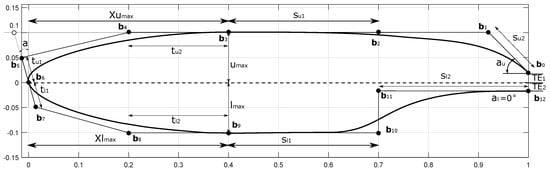
Figure 1.
Foil instance of the parametric model employed in this work. The 17 parameters (marked on the figure above) are used for the parametric definition of the 13 control points determining the foil profile.

Table 1.
Parameters of the employed parametric model. All parameters are defined in .
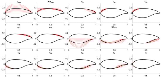
Figure 2.
Effect of the first 15 parametric model parameters on the foil profile. In each subplot, one parameter varies while the others are kept constant. The remaining 2 parameters, and , determine the trailing edge type, i.e., blunt or sharp, and the distance between the two foil sides at the TE.
The incorporation of the parametric model in the development and training of the ANNs used in this work has additional benefits in the behavior of these ML models when predicting the foil shape or its performance. Specifically, as we will demonstrate in Section 3, the parametric model limits the user to producing foil designs that are both valid and within the boundaries of the employed design space, which safeguards us against highly erroneous predictions, which may occur from ML methods [37,38], as well as a design exploration that goes far beyond the training set boundaries [39]. Moreover, it offers an easy way of checking the validity of shapes returned by the inverse design model, since its output must be a valid parametric model shape vector. Another important positive impact coming from the employment of the parametric model is the indirect dimensionality reduction, since we can describe complex shapes with a small set of parameters, and even more importantly, we can do that in a way that does not generate invalid designs in the reduced-dimension design space. This is a clear advantage of our approach, since common dimensionality-reduction techniques cannot eliminate the existence of invalid designs in the latent spaces; see the relevant discussions in [26,40].
2.2. Foil Performance Analysis
The lift and drag coefficients, for each design instance, were estimated with the aid of the well-known XFOIL (https://web.mit.edu/drela/Public/web/xfoil/ accessed on 10 May 2023) computational package, which is a popular tool used in assessing the performance of subsonic airfoils and hydrofoils. XFOIL employs a fast panel method with a fully coupled viscous–inviscid interaction method used in the ISES code developed by Drela and Giles; see [6,41]. XFOIL requires a polygonal approximation of the foil profile, and thus, for each foil design in our dataset, we generated, through the employed parametric model, 200 points that closely approximated the foil’s shape. Specifically, in most cases, 160 points, with a curvature-based distribution that minimizes the distance between the actual curve and the polygonal approximation, sufficed to produce convergent and accurate performance results. However, we decided to increase that number to 200 to avoid inaccuracies and potential problems with more-complex foil profile geometries. A matlab (https://www.mathworks.com/products/matlab.html accessed on 10 May 2023) script was generated to read the design vectors for all foil designs in the dataset, save a polygon approximation, and finally, automatically call XFOIL to compute the lift and drag coefficients for all angles of attack in with a Reynolds number equal to . We should also note here that we increased the viscous solution iteration limit (ITER) in XFOIL so that up to 50 Newton iterations were executed when assessing convergence. This was a significant step, which helped us avoid missing results and non-converging calculations with some more-intricate foil designs. A sample XFOIL output for the calculations described here is depicted in Figure 3. As a final note, we should also add here that a small number of performance calculations (less than 3% of the foil designs in the database) failed for one or two angles of attack. In such cases, we performed a cubic spline interpolation with the remaining and values and estimated the missing value(s) with the resulting spline curve.
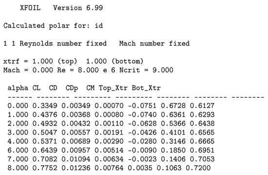
Figure 3.
Example of XFOIL output for a foil instance in the employed dataset. alpha corresponds to the angle of attack, whereas CL and CD correspond to the lift and drag coefficients, respectively.
2.3. Geometric Moments
The geometry and performance information captured by the parameters of the parametric model and the lift/drag coefficients may not be sufficient to fully capture the relation between design and performance, which can result in inadequate regression or generally inaccurate prediction models. In the area of performance-based design optimization, it is not uncommon to embed, in the design vector, information about the quantities of interest and/or incorporate knowledge about the underlying physics in the ML model, as, for example, in the case of physics-informed neural networks; see [31,42,43]. However, these approaches tend to be computationally intensive and require detailed analysis, which imposes an additional computational burden, which is especially unwelcome in the early design stages. Motivated by the work of Shah et al. [26], we attempted to enrich the design and performance description with the integral properties of the foil shape geometry and performance profiles, respectively. Specifically, for the case of the foil’s shape, the geometric information, encoded in the parameters’ vector, was coupled with foil shape moments, leading to an enhanced design vector, which, as will be demonstrated, can offer a more-accurate description of the shape’s inherent characteristics and its relation to the performance metrics. Thus, the incorporation of geometric moments acts as an indirect way of incorporating quantities that are correlated to performance criteria in a cost-effective manner. In other words, while most performance criteria (e.g., lift or drag) require generally costly simulations, these quantities are generally dependent on geometric moments, which can be easily computed with a significantly lower computational cost.
Geometric moments for performance profiles do not necessarily incorporate any inherent information about the foil design, but they can still help the model better predict relations between performance characteristics and the corresponding foil geometry. Therefore, the geometric moments of the lift and drag coefficient profiles were also considered for the inverse design problem.
Assuming now that corresponds to the 2D domain bounded by the foil profile curve , we may compute its -, , order moments by:
where when and 0 otherwise. Obviously, the 2D domain area corresponds to the 0th-order moment, i.e., , and its centroid can be calculated as . A proper combination of geometry and its moments allows the construction of a vector that captures the shape’s inherent characteristics and can serve as its unique identifier, the so-called signature vector in [44].
For the foil profile case, we may compute the Geometric Moments (GMs) with the two-dimensional version of the divergence theorem, i.e., Green’s theorem. Specifically, using Green’s theorem and the representation of the foil profile in (2), we may equivalently write:
and so on.
For the lift and drag coefficient profiles, we constructed a spline interpolating the computed values, and we can then proceed with the calculation of the corresponding moments under the interpolant , where x corresponds to the angle of attack and y to the coefficient values. Note that we used the signed area here, since we may have foil shapes with negative lift coefficients, and therefore, using the signed area would be a more-meaningful performance feature to differentiate between positive- and negative-lift-producing designs. Hence, for the performance profiles, we may calculate the moments as follows:
and so on.
The performance criteria considered in this work, i.e., the lift and drag coefficients, are invariant to translation and uniform scaling, whereas the moments described above change value with Translation (T) and Scaling (S). Therefore, in the general case, we would need to employ TS-invariant Geometric Moments (TS-iGM), as described in Xu and Li in [45] where the authors derived Translation, Scale, and Rotation invariant Geometric Moments (TSR-iGM). However, in our dataset, we only considered foil designs with chords aligned with the longitudinal axis (x-axis), fixed placement, and normalization to [0,1], which permitted us to use the moments derived above without introducing any biases; therefore, we may skip the use of moment invariants.
2.4. Training Datasets
As previously mentioned, the basis for the construction of the foil design space, and subsequently the resulting training datasets, was the publicly available UIUC database of foil designs; see [30]. This database comprises approximately 1500 foil profiles encoded via point sets of varying lengths, i.e., the number of points on the profile. The first step in the construction of the design dataset is a preprocessing step and pertains to ordering points to one common orientation and normalization of the foil shapes so that all of them lie on the x-axis and have a chord length equal to one unit. Subsequently, we determined the parameter values of the foil parametric model, which reconstruct each foil profile within the modified Kulfan tolerance; see Equation (1). This was done by solving the following minimization problem:
where is the number of points, , defining the -th foil in the UIUC database, and are the ordinates of the first and last foil point (Recall that a preprocessing step was performed to ensure that all foil points were stored in a counterclockwise orientation with the first point being the trailing edge point of the upper foil side), respectively.
We solved the minimization problems appearing in Equation (6) using a sequential quadratic programming technique implemented in matlab with an initial design vector resulting from a rough estimation of the design parameters based on the input profile points. This resulted in approximately 1300 design vectors that approximated the corresponding number of foils within the modified Kulfan tolerance. The identified parameter vectors were saved to form the initial design dataset . If we now performed a Principal Component Analysis (PCA) [46] of and use the first two principal components to visualize the designs in , we obtained a picture with isolated designs or clusters of designs with relatively big gaps among them. Although this did not directly correspond to the distance between the high-dimensional design vectors, it provided us with an indicative picture of the distribution of the foil designs in the design space. Additionally, given the number of parameters and performance targets we planned to work with, the number of design vectors was not sufficiently large to ensure a good fit by standard regression or neural network models. To address these issues, we generated 10 design variations in the neighborhood of each design in by varying the identified parameter values around their initial value. In this way, we obtained a significantly larger dataset with fewer gaps between designs, as can been seen by the blue dots in Figure 4. This figure was produced by performing PCA of the augmented set and visualizing both the initial and additional designs (variations) in the same picture with the help of the first two principal components. As one may easily observe in Figure 4, the red circles, corresponding to , are isolated or form clusters of designs with relatively big distances between them, whereas the included variations, blue dots, fill in most gaps and construct a significantly richer dataset that we denote as . The next and final step in the process of design dataset construction was performed with the help of Equation (4) and pertained to the calculation of moments, to , for each design in . These moments were subsequently added to form the final version of .
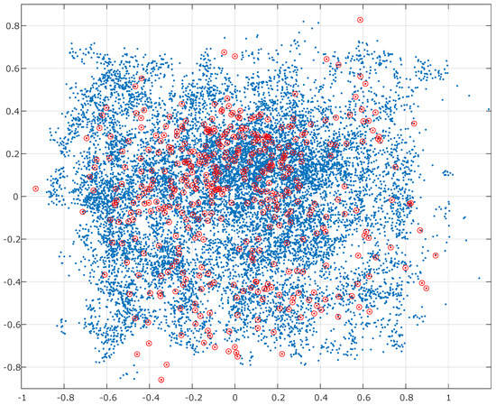
Figure 4.
Foil designs plotted in the 2D design space with coordinates corresponding to the first two principal components; red circles depict the initial UIUC database foil profiles and blue dots the constructed variations.
The initial performance dataset, , was generated by assessing the performance of each design in with XFOIL, as described in Section 2.2, and storing the resulting and values in . As in the case of the design dataset, the performance dataset was augmented with the moments for the performance curves, and , using Equation (5), producing the final performance dataset . We should note here that a small number of designs failed to produce complete performance profiles (cases with more than a couple of and/or values missing), and they were excluded from both and . Therefore, the final datasets, which were used in the regression and training of the neural network models, comprise 12,615 designs with their design vectors and moments in and the corresponding number of performance and performance moment values in . In summary, the matrix structures corresponding to and are depicted in Table 2. We should also note here that we posed certain limitations to the type and number of performance inputs. If we were to use different values or even a different number of angles of attack for each foil design, we would probably need to revert to a Recurrent Neural Network (RNN), which would be able to handle variable-length sequences of inputs. This would become even more important if we were to consider more nuanced performance profiles, including pressure distributions or other low-level performance metrics.
Table 2.
Structure of design and performance datasets.
2.5. Regression Models
For both cases, i.e., forward and inverse design problems, we considered 3 different regression models, which were compared with a range of different training datasets:
- A Multivariate Linear Regression (MLR) [47,48], which constitutes our basis (reference) model;
- Two families of feedforward Artificial Neural Networks (ANNs) trained with (a) Levenberg–Marquardt (LM) back-propagation, and (b) LM with Bayesian Regularization (BR); see Table 3 for more details.
Table 3. Description of forward and inverse regression models. The numbers in curly brackets for the input and output sets correspond to the columns of the datasets and described in Table 2.
As a reference model, for both problems, we employed the multivariate normal regression of either the 18-dimensional performance responses () on the design matrix corresponding to the 17 design parameters (), or vice versa for the inverse design problem. The model is formulated as
where n is the number of samples, 12,615 in our case, is the 18- or 17-dimensional vector of responses, is the design vector of predictor variables, and corresponds to the resulting regression coefficients with denoting the vector of error terms. Note that we added a column of ones in matrix , formed by the 12,615 vectors, to include constant terms (intercepts) in the regression. The root-mean-squared error for the prediction of the performance values with MLR is reported in Table 4, whereas the corresponding MLR error for the inverse problem is found in Table 5.
Table 4.
Performance of forward ANNs and multivariate linear regression in the prediction of the lift and drag coefficients.
Table 5.
Performance of inverse problem ANNs and multivariate linear regression in the prediction of the design parameters.
The remaining models were two-layer feedforward neural networks with an input layer, a hidden layer, and an output layer. For the hidden layers, hyperbolic tangent sigmoid activation functions were used, whereas linear transfer functions were employed in the output layer, as we performed regression in all cases. We should also note here that positive linear (poslin, also known as ReLU—Rectified Linear Unit in the pertinent literature) and logistic sigmoid transfer functions were tested in the hidden layers with inferior results in all tested cases. For the majority of the trained models, we observed that 20 neurons in the hidden layers produced good results, but for some of the employed training datasets, this number was raised to 25 or 30, as can be seen in Table 3. Specifically, we performed model training tests starting with 10 neurons, in the hidden layers, and went up to 70 neurons with a step of 5 neurons. For all cases, the results showed an improvement from 10 to 20 or 30 neurons, followed by a decline in performance after 30 or 35 neurons. As mentioned above, two training approaches were used, LM back-propagation and LM with Bayesian regularization, with “LM” included in the model name in the former case and “BR” for the latter one; see Table 3. Additionally, the scaled conjugate gradient algorithm was used in the training, but we did not include it in our comparisons, as it was outperformed across all tests by the other two training methods.
LM is a standard approach used in training ANNs, and the following steps are applied in its implementation:
- Network weights’ and biases’ initialization.
- Input data are fed into the network, and the activation function values for each neuron in the hidden and output layers are calculated.
- The error between the network’s predicted output and the actual target output is computed using a suitable error metric, the mean-squared error (MSE) in our case.
- The error is then propagated backwards to adjust the weights and biases. For this, the Levenberg–Marquardt algorithm is used to optimize the network parameters. The LM algorithm combines the benefits of fast convergence from the Gauss–Newton algorithm and the robustness of steepest descent. It dynamically adjusts a parameter known as the damping factor during training, controlling the step sizes taken in the weight space.
- The weights and biases of the network are updated using LM.
- Steps 2 to 5 are repeated till convergence has been achieved (or when a maximum number of iterations has been reached).
Bayesian regularization updates the weight and bias values based on the same LM optimization algorithm. It then minimizes a linear combination of squared errors and weights and determines the correct combination so as to produce a network that generalizes well, i.e., does not over-fit the given training data. This was performed by extracting a validation set from the training data and monitoring the model’s performance to prevent over-fitting. Bayes’ theorem was used to combine the prior distributions with the likelihood to obtain the posterior distributions. The linear combination of the squared errors and weights was modified accordingly to achieve good generalization qualities. The interested reader may refer to [49,50] for a more-detailed description of the Bayesian regularization process. We should also note here that an additional test set, separate from the validation set mentioned above and corresponding to 15% of the datasets, was set aside, for all models, and used at the end to confirm the generalization qualities of the trained models. With regard to the training set employed in LM training, a 5-fold cross-validation was utilized to avoid over-fitting. In all cases presented in this work, coefficients of determination, , exceeding 90% for both the training and test sets were achieved. Note that the value reported here for the training set corresponds to the average value from the 5-fold cross-validation.
Before we proceed with the presentation of the achieved results, we need to also briefly discuss the use of different datasets in the training of the models included in Table 3. Specifically, we used a wide range of combinations, starting from the simplest, and , dataset pair, to the full datasets, and , described in Table 2. This was performed to assess the effect of full or partial moments’ inclusion in either the design or performance datasets along with the effect of transferring components from the input to the output sets and vice versa. The area of the foil profile is one such component example, as it can be considered either as the input feature or the output target. Table 3 presents a summary of the trained models along with the composition of the input and output sets that were used for training.
3. Results and Discussion
We begin our presentation with the achieved results and prediction accuracy for the regression models described in the previous section, and we then move on to present two applications employing the best-performing ML models in the preliminary foil design and shape optimization. The first application was a “foil design assistant” software prototype, which can be used by a designer, in the early design stages, to interactively assess the performance of the foil designs he/she intuitively modifies or determine the foil profile that achieves the performance characteristics that he/she may set. The second application demonstrates the use of the developed ML models in foil shape optimization and compares them to the corresponding well-established performance-based shape optimization procedures.
3.1. Regression and ML Models’ Performance
Table 4 summarizes the achieved Root-Mean-Squared Error values (RMSEs) and their normalized counterparts (nRMSEs) for all forward regression models, whereas the corresponding summary for the inverse case is reported in Table 5. The calculation of the RMSE and nRMSE was performed for each model and the performance coefficients, as shown below:
where correspond to the dataset values, to the model-predicted ones, and n to the number of components times the samples in the dataset. One may easily observe from Table 4 that the best-performing model for the case of prediction was the model trained on the full dataset and the -based part of the dataset ( values and moments) with foil areas added also to it. Moreover, the reference model, i.e., multivariate linear regression, was clearly outperformed by all trained ANNs. For the case of prediction, we obtained slightly better results if we excluded the second moments from the input dataset, as can be seen from the same table. However, if we observe Figure 5a,b, which depict the maximum errors in the predictions, we can argue that the best performance was achieved by the “M0-2_BR” model for both the and predictions, as it minimized the maximum error exhibited in the prediction of both performance metrics. Another interesting observation, from the same histograms, is that both the and predictions improved as we inserted more moments in the input descriptors, therefore confirming our hypothesis that the inclusion of geometric moments improves the accuracy of the trained models as it aids in better capturing the relation between design and performance.
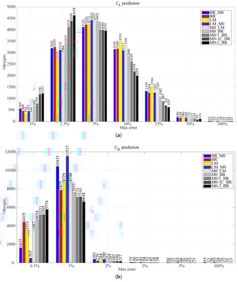
Figure 5.
Histograms of model predictions for the forward foil design problem. (a) Histogram of the max errors in the prediction of the values for all forward ANNs described above. (b) Histogram of the max errors in the prediction of the values for all forward ANNs described in Section 2.5.
However, our results were not that clear when considering the performance of the studied regression models in the inverse design problem. For the inverse problem case, and swapped places, with the former becoming the output set and the latter taking the place of the input set. The first observation pertained to the performance of the reference model, which was only slightly worse when compared to the ANNs, as one may observe in Table 5. Furthermore, the shape prediction accuracy, at least when measured with the maximum deviation in the parameter values, does not look very promising in the histogram in Figure 6a. However, this finding was somewhat misleading, as for example, big differences in a parameter such as the tangent angle at the leading edge (see Table 1 and Figure 2) may result in only slight foil shape differences. If we now take into account such differences in the parameters’ effects, we may use the mean error instead, shown in Figure 6b, which was more representative of the actual foil shape prediction’s accuracy. As in the forward design problem, the inclusion of moments (this time, the moments of the performance curves were considered) had a beneficial effect on the prediction accuracy, but it was not as pronounced as it was for the forward design case. This can be justified by the fact that there was no direct physical correlation between the performance moments and the shape of a foil. Nevertheless, their inclusion had a non-negligible effect in the training process, and they, therefore, helped us achieve a better “discriminatory ability” of the corresponding ANNs.
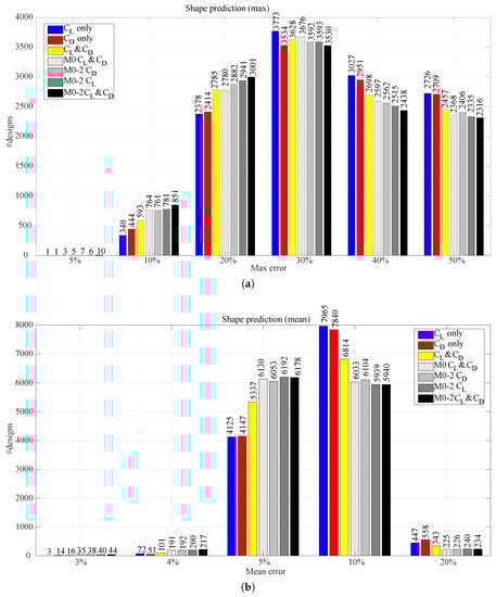
Figure 6.
Histograms of model predictions for the inverse foil design problem. (a) Histogram of the max errors in the prediction of the design variable values for all inverse problem ANNs described in Section 2.5. (b) Histogram of the mean errors in the prediction of the design variable values for all inverse problem ANNs described in Section 2.5.
3.2. Foil Design Assistant
The first application of the identified best-performing ANNs was the design and implementation of a software tool prototype, “FoilDesignAssistant”, which aims to aid designers, in the early design stages, to quickly assess the performance of a wide range of foil shapes and/or identify the foil shape that possesses the performance criteria set by them. The objectives set for this tool were as follows:
- Provide an interactive and intuitive interface for modifying a foil’s profile.
- Assess in real-time the foil’s performance characteristics.
- Compare the initial and modified design with respect to their performance characteristics.
- Provide an interactive and intuitive interface for defining a foil’s performance characteristics.
- Determine in real-time the foil profile that exhibited the user-defined foil performance characteristics.
- Limit the user input to information that is commonly available at the early design stages.
Figure 7 depicts the interface of the prototype software application developed in matlab. The tool aids the designer in both foil design cases, i.e., forward and inverse problems, using the ML models that were previously identified for their fidelity, i.e., the pair of M0-2_BR ANNs for the prediction of and and M0, M0-2_ (M0-2) for the foil design parameters’ identification. The mode of operation is determined by the “design mode” check button depicted below the “Foil” design window in Figure 7. When this button is checked, the forward problem is considered, whereas when it is unchecked, the model for the inverse design problem is employed. The interface comprises three graph components: (a) the “Foil” graph (upper left corner in Figure 7, (b) the “Lift Coefficient” graph (upper right side in Figure 7), and (c) the “Drag Coefficient” graph below it in the same figure. Below the “Foil” graph, a series of sliders corresponding to the parameters of the employed parametric model are presented, whereas the input fields for defining the required performance characteristics are placed below the performance graphs at the right side. Additionally, a drop-list button below the “Drag Coefficient” graph is used to initialize the current design into one of the well-known foil designs (e.g., NACA family profiles and others) and an export functionality at the lower right part of the interface. The export function allows saving the current design (blue-colored design) as a NURBS curve or a point set with a user-selected number of points and discretization type. We subsequently describe the software tool’s operation in the two modes:
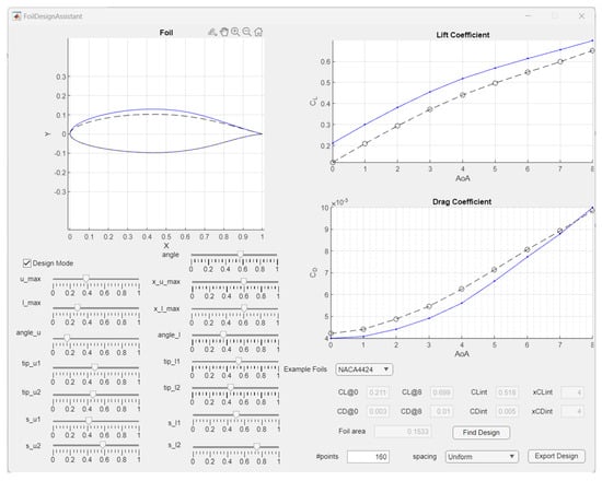
Figure 7.
Foil Design Assistant application, main interface.
- Forward design mode: The user interactively modifies the foil design by adjusting the parametric model parameter values via the sliders on the interface window. These parameters correspond to the already-described parameters in Table 1. Whenever a user modifies a value, the current design (blue curve) is updated in all graphs in real-time. At the same time, the initial design (black curve) is depicted in all graphs for facilitating the comparisons. Note here that the user only specifies the foil parametric model parameters, while all moments required as the input to the M0-2_BR model are automatically calculated via the parametric model embedded in the application.
- Inverse design mode: In this mode, the user may specify one or all of the input fields residing on the right side of the interface. Specifically, CL0 and CD0 are used to specify the desired values of and at a 0°angle of attack, while CL8 and CD8 specify the desired values of the same coefficients at an 8°angle of attack for the sought-for foil profile. Furthermore, an intermediate performance point at the xCLint angle for and xCDint for may by provided, with the corresponding coefficient values being specified in CLint and CDint, respectively. Finally, the user may also specify the desired foil area using the “Foil area” input field. As soon as the user clicks on the “Find Design” button, two splines using the specified points for the and performance profiles are computed, and the results are fed into the inverse ML model, along with the foil area and all required performance profile moments. Similar to the forward design mode, all graphs are updated in real-time with the current design being depicted with blue color and the initial one with black.
Based on the description above, we satisfied (a) the requirement of interactivity by automatically, and in real-time, updating all relevant information and graphs, (b) the requirement of intuitiveness by employing the high-level parameters, with physical meaning, for the determination of the profile design, and finally, (c) the accuracy objective achieved by incorporating the best-performing ML models for both design problems. As a final note, we need to also mention here that one may easily substitute the ML models employed in the tool with any of the models presented in Section 2.5, and the required collection of user-determined input and output, along with the calculation of additional moments, is automatically adjusted to match the requirements of selected models, as described in Table 3.
3.3. Foil Shape Optimization
In this subsection, a comparison between a traditional performance-based shape optimization approach and the optimization setup enabled by the trained ANNs is presented. For this comparison, we intentionally picked an initial design for which the trained models provided a relative inaccurate performance prediction, as can be seen in Figure 8b. As one can observe in Figure 5b, the max error in the prediction for the great majority of the designs was below 2%, whereas for the selected design, it reached 20% or even above. Specifically, we considered a one-meter chord length foil design (ID7910) with a sharp trailing edge (TE at ), which is defined by the initial design vector, , shown in Table 6. The corresponding foil profile shape is depicted in Figure 8a. Furthermore, we considered that the foil operates at a 3°angle of attack with a Reynolds number equal to , and we aimed to maximize the lift-over-drag ratio while maintaining a constant foil area. Finally, we limited the design space by permitting a maximum parameter value deviation (Each parameter value lies in , and hence, corresponds to ) of around the initial value for each parameter. Therefore, the shape optimization problem can be formulated as follows:
where is the allowable deviation from the initial enclosed area of the selected foil profile (ID7910).
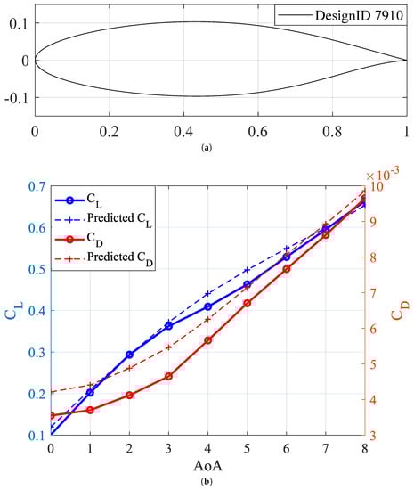
Figure 8.
Selected design for optimization along with the corresponding lift (blue) and drag (red) coefficients for an angle of attack range in . (a) Foil shape; (b) and performance—actual and predicted.
Table 6.
Design parameters for the initial and optimized designs.
In the traditional performance-based shape optimization approach, we used the employed parametric model for generating foil design instances using a design vector with the model’s first 15 parameters; recall that we considered a sharp trailing edge at , and therefore, . The lift and drag coefficients, for each design instance, were once again estimated with the aid of the well-known XFOIL computational package (https://web.mit.edu/drela/Public/web/xfoil/ accessed on 10 May 2023), which, as mentioned previously, is a popular tool used in assessing the performance of subsonic airfoils. XFOIL employs a fast panel method with a fully coupled viscous/inviscid interaction method used in the ISES code developed by Drela and Giles; see also [6,41]. Obviously, when the trained ANNs are employed, no simulations are necessary, but we may still need to use the parametric model for the moments’ calculation. Specifically, in this benchmark example, we employed the M0-2_BR ANN, which produced the most-accurate prediction results; see Table 4 and Figure 5. The optimization algorithm employed for both cases was Pattern Search [51,52,53], a derivative-free global optimization algorithm, with the initial design (ID7910) being its starting point for both cases.
Figure 9 depicts the initial design (thin dashed line) along with the resulting optimized foil shapes for the traditional performance-based shape optimization with XFOIL (thick solid line) and the ML-enabled shape optimization (thick dashed line). The two optimized designs, although not identical, were well aligned and differed only slightly overall, with a more-visible deviation at the aft part of the upper foil side. In Table 7, we report the parametric model parameters corresponding to the initial design (Row 1) and the two optimized profiles in Rows 2 (traditional) and 3 (ML-based). One may easily observe from the same table that the difference between the two optimized designs was mainly in the parameters and , which, as expected, affected the part, which is visibly different between the two shapes. Performancewise, the shape resulting from the traditional optimization approach exhibited better performance, whereas the result from the ML-enabled optimization, although significantly improved when compared to the initial design, lacked slightly in performance when compared to the former optimized design. We summarize these results in Table 7, where the lift and drag coefficients along with the ratio, foil area, and required computational time are reported for each case. Note that all results in this table were evaluated with XFOIL so that they are directly comparable. The ML-enabled optimization achieved a 42.3% increase in lift followed by a small (4.58%) increase in drag, which resulted in a 26.5% improvement of the drag-to-lift ratio. The traditional approach outperformed these results, with the corresponding values being 57.9%, 1.92%, and 35.6%, respectively. However, if we look at the last column in Table 7, we can see where the ML-based approach really shined. Specifically, the computation time required dropped by approximately 85% when compared to the traditional approach. In addition, if one observes the parameter values identified by the ML-based approach in Table 6, we can easily assume that, by running a fast gradient-based optimization algorithm, such as steepest descent or Newton’s method, we may acquire the results achieved by the traditional optimization approach. Indeed, we used matlab’s fmincon function with the Sequential Quadratic Programming algorithm and reached the traditional approach’s results in just two iterations. Therefore, in summary, the ML-based approach can achieve relatively accurate and comparable (or even identical results, if we apply a secondary optimization step) with only of the computational time required for the traditional approach, and this, as indicated in this example, occurred even when we started from a design that was not accurately captured by the trained ANN model.
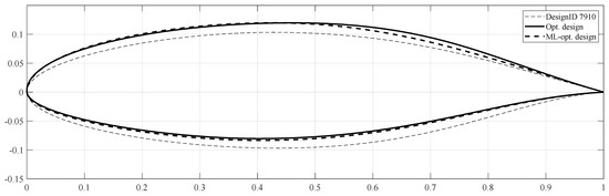
Figure 9.
Optimized foil profiles compared with the initial design (thin dashed line). The ML-based optimization result is depicted with a thick dashed line, while the optimized design using XFOIL is depicted with a thick solid line.
Table 7.
Design optimization results.
4. Conclusions and Future Work
In this work, we demonstrated a successful application of Artificial Neural Network models in the forward and inverse foil design problems for early foil design stages. This was accomplished by integrating a foil parametric model for an intuitive, accurate, and compact representation of foil designs and an appropriately prepared rich dataset of realistic foil designs. The incorporation of the parametric model in the development of the model served also as a safeguard against invalid input, highly inaccurate predictions, and design exploration that went far beyond the training dataset. Specifically, the parametric model was constructed in way that guaranteed the construction of valid foil shapes for the complete range of its parameter values with the employed instances distributed in the design space, as indicated in Figure 4. At the same time, the output of the models used in the inverse design problem needed to produce valid shape vectors, which permitted us to easily identify erroneous predictions. In addition, geometric moments were incorporated in both the input and output datasets and were shown to significantly improve the accuracy of the ANNs in the prediction of the foil’s performance. Similarly, the inclusion of performance moments was shown to enhance the predictions for the inverse design problem, although their effect was less pronounced. The developed ANNs were compared against a reference linear regression model to benchmark their performance, and a wide range of variations with regard to their training procedure and the composition of the training datasets was examined to identify the best-performing models. Finally, the best-performing models were used to demonstrate the proposed approach in a real-time, intuitive “foil design assistant” software prototype, with a performance-based shape optimization example. The results obtained from the ML-enabled shape optimization were comparable to the traditional foil shape optimization approaches with the additional benefit of requiring only a fraction of the time needed for traditional approaches.
Although we demonstrated good prediction accuracy with the developed procedures, there were several limitations that we would need to address in the future. One of these limitations pertained to the usage of fixed performance metrics, i.e., the lift and drag coefficients for a fixed number of angles of attack, which limited the applicability of our approach to the early design stages. We could potentially employ recurrent neural networks and/or 1D convolutional neural networks to include variable-sized performance input and lower-level performance metrics, such as pressure distributions, which would expand the applicability of our approach beyond the early design stages. In a similar manner, the assessment of foil performance using panel methods was a restrictive limitation in our work, as it was noted in the introductory section. As we have now established the beneficial impact of the geometric moments’ inclusion, as well as the dimensionality reduction and robustness, which was attributed to the employed parametric model, we may move forward and include high-fidelity CFD simulations for the foil performance assessment, which would obviously expand the applicability of the proposed design tools. Moreover, we plan to conduct a study in the near future regarding the use of the developed Foil Design Assistant to assess its impact on the design effectiveness of students and professionals assigned foil design assessment and optimization tasks. Finally, we plan to extend this approach for the 3D case with wind turbine and propeller blades being the next possible objects of interest. Apart from the obvious tasks of extending the type of ML models and constructing appropriate datasets, the inclusion of geometric moment invariants should be also considered to alleviate the need for fixed placements and design normalization, which might not be possible for general functional surfaces.
Author Contributions
Conceptualization, K.V.K.; methodology, K.V.K. and M.M.; software, K.V.K. and M.M.; validation, K.V.K. and M.M.; formal analysis, K.V.K.; resources, K.V.K.; data curation, K.V.K. and M.M.; writing—original draft preparation, K.V.K. and M.M.; writing—review and editing, K.V.K. and M.M.; supervision, K.V.K.; project administration, K.V.K.; funding acquisition, K.V.K. All authors have read and agreed to the published version of the manuscript.
Funding
This work received funding from Nazarbayev University, Kazakhstan, under the Faculty Development Competitive Research Grants Program 2022–2024: “Shape Optimization of Free-form Functional surfaces using isogeometric Analysis and Physics-Informed Surrogate Models—SOFFA-PHYS”, Grant Award No. 11022021FD2927.
Institutional Review Board Statement
Not applicable.
Informed Consent Statement
Not applicable.
Data Availability Statement
The raw data required to reproduce the findings in this work and the software application are available from Dr. Konstantinos Kostas, upon email request (konstantinos.kostas@nu.edu.kz).
Conflicts of Interest
The authors declare no conflict of interest. The funders had no role in the design of the study; in the collection, analyses, or interpretation of the data; in the writing of the manuscript; nor in the decision to publish the results.
References
- Harries, S.; Abt, C.; Brenner, M. Upfront CAD—Parametric modeling techniques for shape optimization. In Advances in Evolutionary and Deterministic Methods for Design, Optimization and Control in Engineering and Sciences; Springer: Cham, Switzerland, 2019; pp. 191–211. [Google Scholar]
- Kostas, K.; Ginnis, A.; Politis, C.; Kaklis, P. Ship-hull shape optimization with a T-spline based BEM–isogeometric solver. Isogeometric Analysis Special Issue. Comput. Methods Appl. Mech. Eng. 2015, 284, 611–622. [Google Scholar] [CrossRef]
- Masters, D.A.; Poole, D.J.; Taylor, N.J.; Rendall, T.; Allen, C.B. Impact of Shape Parameterisation on Aerodynamic Optimisation of Benchmark Problem. In Proceedings of the 54th AIAA Aerospace Sciences Meeting, San Diego, CA, USA, 4–8 January 2016. [Google Scholar] [CrossRef]
- Masters, D.A.; Taylor, N.J.; Rendall, T.C.S.; Allen, C.B.; Poole, D.J. Geometric Comparison of Aerofoil Shape Parameterization Methods. AIAA J. 2017, 55, 1575–1589. [Google Scholar] [CrossRef]
- Hess, J.; Smith, A. Calculation of potential flow about arbitrary bodies. Prog. Aerosp. Sci. 1967, 8, 1–138. [Google Scholar] [CrossRef]
- Drela, M.; Giles, M. Viscous-inviscid analysis of transonic and low Reynolds number airfoils. AIAA J. 1987, 25, 1347–1355. [Google Scholar] [CrossRef]
- Lee, C.; Kerwin, J. A B-spline higher-order panel method applied to two-dimensional lifting problem. J. Ship Res. 2003, 47, 290–298. [Google Scholar] [CrossRef]
- Kim, G.; Lee, C.; Kerwin, J. A B-spline based higher-order panel method for the analysis of steady flow around marine propellers. Ocean. Eng. 2007, 34, 2045–2060. [Google Scholar] [CrossRef]
- Gao, Z.; Zou, Z. A NURBS based high-order panel method for three-dimensional radiation and diffraction problems with forward speed. Ocean. Eng. 2008, 35, 1271–1282. [Google Scholar] [CrossRef]
- Kostas, K.; Ginnis, A.; Politis, C.; Kaklis, P. Shape-optimization of 2D hydrofoils using an Isogeometric BEM solver. Comput.-Aided Des. 2017, 82, 79–87. [Google Scholar] [CrossRef]
- Chouliaras, S.; Kaklis, P.; Kostas, K.; Ginnis, A.; Politis, C. An Isogeometric Boundary Element Method for 3D lifting flows using T-splines. Comput. Methods Appl. Mech. Eng. 2021, 373, 113556. [Google Scholar] [CrossRef]
- Katz, J.; Plotkin, A. Low-Speed Aerodynamics, 2nd ed.; Cambridge Aerospace Series; Cambridge University Press: Cambridge, UK, 2001. [Google Scholar] [CrossRef]
- Versteeg, H.; Malalasekera, W. An Introduction to Computational Fluid Dynamics: The Finite Volume Method, 2nd ed.; Pearson: London, UK, 2007. [Google Scholar]
- Smith, M.J.C.; Wilkin, P.J.; Williams, M.H. The Advantages of an Unsteady Panel Method in Modelling the Aerodynamic Forces on Rigid Flapping Wings. J. Exp. Biol. 1996, 199, 1073–1083. [Google Scholar] [CrossRef]
- Shen, H.; Liu, Y.; Chen, B.; Lu, Y. Control-relevant modeling and performance limitation analysis for flexible air-breathing hypersonic vehicles. Aerosp. Sci. Technol. 2018, 76, 340–349. [Google Scholar] [CrossRef]
- Wang, S.; González-Cao, J.; Islam, H.; Gómez-Gesteira, M.; Guedes Soares, C. Uncertainty estimation of mesh-free and mesh-based simulations of the dynamics of floaters. Ocean. Eng. 2022, 256, 111386. [Google Scholar] [CrossRef]
- Mishra, A.A.; Mukhopadhaya, J.; Iaccarino, G.; Alonso, J. Uncertainty Estimation Module for Turbulence Model Predictions in SU2. AIAA J. 2019, 57, 1066–1077. [Google Scholar] [CrossRef]
- Hui, X.; Bai, J.; Wang, H.; Zhang, Y. Fast pressure distribution prediction of airfoils using deep learning. Aerosp. Sci. Technol. 2020, 105, 105949. [Google Scholar] [CrossRef]
- Wang, L.; Xu, J.; Luo, W.; Luo, Z.; Xie, J.; Yuan, J.; Tan, A.C. A deep learning-based optimization framework of two-dimensional hydrofoils for tidal turbine rotor design. Energy 2022, 253, 124130. [Google Scholar] [CrossRef]
- Du, Q.; Liu, T.; Yang, L.; Li, L.; Zhang, D.; Xie, Y. Airfoil design and surrogate modeling for performance prediction based on deep learning method. Phys. Fluids 2022, 34, 015111. [Google Scholar] [CrossRef]
- Li, J.; Du, X.; Martins, J.R. Machine learning in aerodynamic shape optimization. Prog. Aerosp. Sci. 2022, 134, 100849. [Google Scholar] [CrossRef]
- Kharal, A.; Saleem, A. Neural networks based airfoil generation for a given Cp using Bezier–PARSEC parameterization. Aerosp. Sci. Technol. 2012, 23, 330–344. [Google Scholar] [CrossRef]
- Sobieczky, H. Parametric Airfoils and Wings. In Recent Development of Aerodynamic Design Methodologies. Notes on Numerical Fluid Mechanics; Fujii, K., Dulikravich, G., Eds.; Springer Vieweg+Teubner Verlag: Berlin, Germany, 1999; Volume 65. [Google Scholar]
- Derksen, R.; Rogalsky, T. Bezier-PARSEC: An optimized aerofoil parameterization for design. Adv. Eng. Softw. 2010, 41, 923–930. [Google Scholar] [CrossRef]
- Diez, M.; Campana, E.F.; Stern, F. Design-space dimensionality reduction in shape optimization by Karhunen–Loève expansion. Comput. Methods Appl. Mech. Eng. 2015, 283, 1525–1544. [Google Scholar] [CrossRef]
- Khan, S.; Kaklis, P.; Serani, A.; Diez, M.; Kostas, K. Shape-supervised Dimension Reduction: Extracting Geometry and Physics Associated Features with Geometric Moments. Comput.-Aided Des. 2022, 150, 103327. [Google Scholar] [CrossRef]
- Chen, W.; Chiu, K.; Fuge, M.D. Airfoil design parameterization and optimization using Bézier generative adversarial networks. AIAA J. 2020, 58, 4723–4735. [Google Scholar] [CrossRef]
- Du, X.; He, P.; Martins, J.R. A B-spline-based generative adversarial network model for fast interactive airfoil aerodynamic optimization. In Proceedings of the AIAA Scitech 2020 Forum, Orlando, FL, USA, 6–10 January 2020; p. 2128. [Google Scholar]
- Li, J.; Bouhlel, M.A.; Martins, J.R. Data-based approach for fast airfoil analysis and optimization. AIAA J. 2019, 57, 581–596. [Google Scholar] [CrossRef]
- UIUC Applied Aerodynamics Group. UIUC Airfoil Coordinates Database. 2023. Available online: https://m-selig.ae.illinois.edu/ads/coord_database.html (accessed on 10 February 2023).
- Sun, Y.; Sengupta, U.; Juniper, M. Physics-informed deep learning for simultaneous surrogate modeling and PDE-constrained optimization of an airfoil geometry. Comput. Methods Appl. Mech. Eng. 2023, 411, 116042. [Google Scholar] [CrossRef]
- Oshima, E.; Lee, N.; Gharib, M.; Lee, V.; Khodadoust, A. Development of a physics-informed neural network to enhance wind tunnel data for aerospace design. In Proceedings of the AIAA SCITECH 2023 Forum, National Harbor, MD, USA, 23–27 January 2023. [Google Scholar] [CrossRef]
- Kostas, K.; Amiralin, A.; Sagimbayev, S.; Massalov, T.; Kalel, Y.; Politis, C. Parametric model for the reconstruction and representation of hydrofoils and airfoils. Ocean. Eng. 2020, 199, 107020. [Google Scholar] [CrossRef]
- Kulfan, B.; Bussoletti, J. Fundamental Parametric Geometry Representations for Aircraft Component Shapes. In Proceedings of the 11th AIAA/ISSMO Multidisciplinary Analysis and Optimization Conference, Portsmouth, VA, USA, 6–8 September 2006. [Google Scholar]
- Kulfan, B.M. Universal Parametric Geometry Representation Method. J. Aircr. 2008, 45, 142–158. [Google Scholar] [CrossRef]
- Piegl, L.; Tiller, W. The Nurbs Book, 2nd ed.; Springer: Berlin/Heidelberg, Germany, 1997. [Google Scholar]
- Nguyen, A.; Yosinski, J.; Clune, J. Deep neural networks are easily fooled: High confidence predictions for unrecognizable images. In Proceedings of the 2015 IEEE Conference on Computer Vision and Pattern Recognition (CVPR), Boston, MA, USA, 7–12 June 2015; pp. 427–436. [Google Scholar] [CrossRef]
- Mishra, A.A.; Edelen, A.; Hanuka, A.; Mayes, C. Uncertainty quantification for deep learning in particle accelerator applications. Phys. Rev. Accel. Beams 2021, 24, 114601. [Google Scholar] [CrossRef]
- Lakshminarayanan, B.; Pritzel, A.; Blundell, C. Simple and Scalable Predictive Uncertainty Estimation Using Deep Ensembles. In Proceedings of the 31st International Conference on Neural Information Processing Systems, NIPS’17, Long Beach, CA, USA, 4–9 December 2017; pp. 6405–6416. [Google Scholar]
- Khan, S.; Goucher-Lambert, K.; Kostas, K.; Kaklis, P. ShipHullGAN: A generic parametric modeller for ship hull design using deep convolutional generative model. Comput. Methods Appl. Mech. Eng. 2023, 411, 116051. [Google Scholar] [CrossRef]
- Drela, M. XFOIL: An Analysis and Design System for Low Reynolds Number Airfoils. In Low Reynolds Number Aerodynamics; Mueller, T., Ed.; Lecture Notes in Engineering; Springer: Berlin/Heidelberg, Germany, 1989; Volume 54. [Google Scholar]
- Ang, E.; Ng, B.F. Physics-Informed Neural Networks for Flow Around Airfoil. In Proceedings of the AIAA SCITECH 2022 Forum, San Diego, CA, USA, 3–7 January 2022. [Google Scholar] [CrossRef]
- Wong, B.; Damodaran, M.; Khoo, B.C. Physics-Informed Machine Learning for Inverse Airfoil Shape Design. In Proceedings of the AIAA AVIATION 2023 Forum, San Diego, CA, USA, 12–16 June 2023. [Google Scholar] [CrossRef]
- Bronstein, A.M.; Bronstein, M.M.; Kimmel, R. Numerical Geometry of Non-Rigid Shapes; Springer: Berlin/Heidelberg, Germany, 2008. [Google Scholar]
- Xu, D.; Li, H. Geometric moment invariants. Pattern Recognit. 2008, 41, 240–249. [Google Scholar] [CrossRef]
- Jolliffe, I.T. Principal Component Analysis, 2nd ed.; Springer: Berlin/Heidelberg, Germany, 2006. [Google Scholar] [CrossRef]
- Little, R.J.A.; Rubin, D.B. Statistical Analysis with Missing Data, 3rd ed.; Seriers in Probability and Statistics; Wiley: Hoboken, NJ, USA, 2019. [Google Scholar]
- Meng, X.L.; Rubin, D.B. Maximum likelihood estimation via the ECM algorithm: A general framework. Biometrika 1993, 80, 267–278. [Google Scholar] [CrossRef]
- MacKay, D.J.C. Bayesian Interpolation. Neural Comput. 1992, 4, 415–447. [Google Scholar] [CrossRef]
- Dan Foresee, F.; Hagan, M. Gauss-Newton approximation to Bayesian learning. In Proceedings of the International Conference on Neural Networks (ICNN’97), Houston, TX, USA, 12 June 1997; Volume 3, pp. 1930–1935. [Google Scholar] [CrossRef]
- Audet, C.; Dennis, J.E. Analysis of Generalized Pattern Searches. SIAM J. Optim. 2002, 13, 889–903. [Google Scholar] [CrossRef]
- Lewis, R.M.; Torczon, V. A Globally Convergent Augmented Lagrangian Pattern Search Algorithm for Optimization with General Constraints and Simple Bounds. SIAM J. Optim. 2002, 12, 1075–1089. [Google Scholar] [CrossRef]
- Lewis, R.M.; Shepherd, A.; Torczon, V. Implementing Generating Set Search Methods for Linearly Constrained Minimization. SIAM J. Sci. Comput. 2007, 29, 2507–2530. [Google Scholar] [CrossRef]
Disclaimer/Publisher’s Note: The statements, opinions and data contained in all publications are solely those of the individual author(s) and contributor(s) and not of MDPI and/or the editor(s). MDPI and/or the editor(s) disclaim responsibility for any injury to people or property resulting from any ideas, methods, instructions or products referred to in the content. |
© 2023 by the authors. Licensee MDPI, Basel, Switzerland. This article is an open access article distributed under the terms and conditions of the Creative Commons Attribution (CC BY) license (https://creativecommons.org/licenses/by/4.0/).