Hydrodynamic Characteristic Analysis and NSGA-II Optimization of a Vacuum Fish Pump

Abstract

The fish pump is an important piece of power equipment for aquaculture, especially for deep-sea engineering vessels and cage culture. Fish pump research focuses on reducing fish body damage, improving survival rates, and increasing fish lifting efficiency. The research object in this paper is a new type of vacuum fish pump, with the aim of improving the hydraulic performance of the vacuum fish pump and reducing the damage to the fish body. The dependent variables include the dynamic change process of the flow state and flow field under diachronic conditions, the fluid simulation analysis of the vacuum pump body and the flow channel structure, the inlet flow rate of the fish pump, the negative pressure of the pipeline, and the impact force of the water flow on the inner wall of the tank. The independent variables include the operating conditions of the pump body and the fish pump. The Latin hypercube sampling method is used to extract 167 sets of calculation models for the independent variables, and multi-objective optimization is performed based on the NSGA-II algorithm for the hydrodynamic performance of the fish pump. On the basis of ensuring the fish body damage rate, the structural parameters of the vacuum fish pump with the optimal hydrodynamic performance under 167 sets of parameter values were obtained. The optimized parameters were then entered into the solver again, and the results showed that, in the optimal structural parameters under certain conditions, the direction of the incident water flow in the vacuum fish pump tank is close to the upper end of the tank body, which will reduce the speed of the fish-water mixed flow when entering the tank, thereby reducing the collision damage to the fish body. Currently, the water flow velocity at the water inlet is about 2.5 m/s, and the negative pressure value distribution gradient between the tank body and the water inlet pipeline is quite consistent, which can achieve good fish suction and fish lifting effects.

1. Introduction

It is difficult for the traditional methods and catch-and-catch methods to meet the actual needs of field operations with the development of the aquaculture industry, particularly with the emergence of large-scale deep-water cages, deep-sea farming boats, and other fish farming models [1]. Therefore, achieving the mechanization and automation of fish captures as well as guaranteeing the catch’s survival and non-damage rate is an important topic in the research field of fishery catch equipment [2]. The fish pump is becoming a research hot spot for many domestic scholars as a key piece of equipment to improve the mechanization level of aquaculture. There are various forms of fish pumps, including vacuum pumps, centrifugal impeller pumps, jet pumps, etc. In-depth research has been conducted, and the design and research process of the fish pump has been focused on protecting the fish body from harm, increasing the fish body’s survival rate, and increasing the fishing efficiency [3].

The design and development of the fish pump needs to focus on solving the problems of lossless fish body transmission, enhancing adaptability, improving intelligence levels, and establishing continuous fishing systems for pelagic fisheries. Tian Changfeng [4], based on the structural characteristics of single-channel pumps, summarized the design methods of single-channel pumps through a large number of experimental studies and design practices and analyzed the structure of single-channel pump impellers and the reasons for their excellent non-clogging performance. They then proposed a new method for improving the hydraulic design of single-channel pumps. Summerfelt [5] used 3D design software to make a solid model of the fish pump and presented the local details, which laid the foundation for the subsequent design and manufacture of the fish pump. Chu Shupo [6] explored the effect of the volute structure on the performance of the fish pump, studied the characteristics of the pump’s internal flow field, and analyzed the effect of the control law of the vacuum outlet form on its performance. Ding Ziyang [7] and Zhang Liang [8] analyzed the pressure and velocity distribution inside the fish as well as the trajectory of the trace in the pump. Numerous scholars have also conducted extensive research on the analysis of the hydrodynamic characteristics of structures. Dutta [9] used the open-source computational fluid dynamics (CFD) modeling tool REEF3D to simulate the oscillatory flow, and the CFD model solves the Reynolds–Averaged Navier–Stokes (RANS) equations in all three dimensions. Further analysis was conducted using CFD to study the effect of blockage ratio on the hydrodynamic characteristics of different oscillatory flow regimes. Dutta [10] used three-dimensional simulations to investigate scour in combined wave-current flows around rectangular piles with various aspect ratios. The simulation model solved the RANS equations using the k–ω turbulence model and included the Exner equation to compute bed elevation changes. The model also used the level-set approach to accurately capture the free surface and included a hydrodynamic module with a morphological module to simulate the scour process.

The currently used fish pump has problems such as a high fish body damage rate, low efficiency, a bulky body, and high energy consumption. This paper aims at improving the hydrodynamic performance of the vacuum fish pump. CFD analysis entails performing fluid simulation analysis on the vacuum pump body and flow channel structure as well as conducting research on the working conditions of fish suction and analyzing the flow field, pressure, speed, and numerical simulation parameters in the flow channel. The dependent variables include the hydrodynamic performance of the fish pump and the influence of fish body damage, the inlet flow velocity of the fish pump, the negative pressure of the pipeline, and the impact force of the water flow on the inner wall of the tank. The independent variables include the working environment of the pump body and the fish pump. The structural form of the fish pump with the optimum performance is obtained using the multi-objective optimization of the fish pump based on the particle swarm optimization algorithm.

2. Overview of Design Scheme

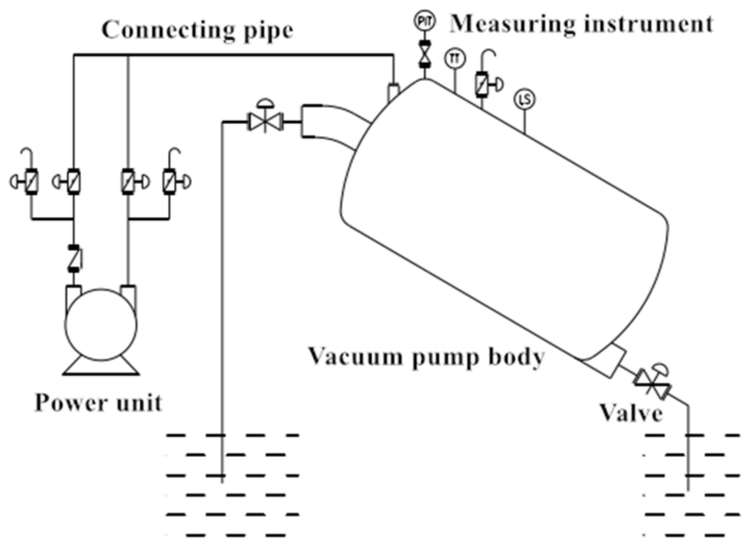
Taking a vacuum fish pump as the research object, Figure 1 depicts the specific structure of this type of vacuum fish pump. The structure of the vacuum fish pump is mainly composed of a power unit, a vacuum pump body, and connecting pipes. The vacuum pump body is the basic unit of the fish-sucking pump structure, and it causes less harm to the fish body when sucking fish [11]. The fluid simulation analysis of the vacuum pump body and the flow channel structure is conducted using the standard turbulent flow model and the Euler multiphase flow method. Additionally, the fish suction working condition is studied, and the flow field, pressure, velocity, and numerical simulation parameters in the flow channel are analyzed. Taking the impact on the hydrodynamic performance of the vacuum fish pump, the inlet flow rate of the fish pump, the negative pressure of the pipeline, and the impact force of the water flow on the inner wall of the tank as the dependent variables, the tank volume, the diameter of the water inlet, and the exhaust speed are selected. The diameter of the mouth, the height, and the angle of the pump body are taken as independent variables, and the multi-objective optimization of the fish pump based on the particle swarm algorithm is used to analyze and obtain the optimal structure of the fish pump.

3. Basis of Theoretical Analysis

In this paper, we use the commercial computational fluid dynamics software ANSYS fluent for finite element (FEM) analysis and calculation. The Eulerian multiphase model in ANSYS Fluent allows for the modeling of multiple separate yet interconnected phases. The phases can be liquids, gases, or solids in nearly any combination. In contrast to the discrete phase model, each phase receives a Eulerian treatment. The number of secondary phases in the Eulerian multiphase model is exclusively limited by memory needs and convergence behavior. As long as sufficient memory is available, any number of secondary phases can be modeled.

3.1. Volume Fraction Equation

The description of multiphase flow as interpenetrating continua incorporates the concept of phasic volume fractions, denoted here by ${\alpha }_q$. Volume fractions represent the space occupied by each phase, and the laws of conservation of mass and momentum are satisfied by each phase individually. The derivation of the conservation equations can be executed by ensemble averaging the local instantaneous balance for each of the phases or by using the mixture theory approach. The volume of phase $q$, $V_q$ is defined by:

$$V_q={\displaystyle {\int }_V{\alpha }_q}dV$$

(1)

where:

$${\displaystyle \sum _{q=1}^n{\alpha }_q}=1$$

(2)

The effective density of the phase $q$ is:

$$\widehat{\rho }={\alpha }_q{\rho }_q$$

(3)

where ${\rho }_q$ is the physical density of phase $q$, ${\alpha }_q$ is the volume fraction of phase $q$.

The volume fraction equation may be solved either through implicit or explicit time discretization.

3.2. Conservation Equations

This section presents the general conservation equations from which the equations are derived, followed by the solved equations.

3.2.1. Conservation of Mass

The continuity equation for phase $q$ is:

$$\frac{\partial }{\partial t}({\alpha }_q{\rho }_q)+\nabla ({\alpha }_q{\rho }_q{\overrightarrow{v}}_q)={\displaystyle \sum _{p=1}^n({\dot{m}}_{pq}-{\dot{m}}_{qp})}+S_q$$

(4)

where ${\overrightarrow{v}}_q$ is the velocity of phase $q$ and ${\dot{m}}_{pq}$ characterizes the mass transfer from the $p^{th}$ to $q^{th}$ phase, and ${\dot{m}}_{pq}$ characterizes the mass transfer from phase $q$ to phase $p$, and you are able to specify these mechanisms separately.

By default, the source term $S_q$ on the right-hand side of Equation (4) is zero, but it can specify a constant or user-defined mass source for each phase. A similar term appears in the momentum and enthalpy equations.

3.2.2. Conservation of Momentum

The momentum balance for phase $q$ yields:

$$\begin{array}{ll}\frac{\partial }{\partial t}({\alpha }_q{\rho }_q{\overrightarrow{v}}_q)+\nabla ({\alpha }_q{\rho }_q{\overrightarrow{v}}_q{\overrightarrow{v}}_q)=& -{\alpha }_q\nabla p+\nabla •{\stackrel{=}{\tau }}_q+{\alpha }_q{\rho }_q\overrightarrow{g}\\ & +{\displaystyle \sum _{p=1}^n({\overrightarrow{R}}_{pq}+{\dot{m}}_{pq}{\overrightarrow{v}}_{pq}-{\dot{m}}_{qp}{\overrightarrow{v}}_{qp})}\\ & +({\overrightarrow{F}}_q+{\overrightarrow{F}}_{\mathrm{lift},q}+{\overrightarrow{F}}_{\mathrm{wl},q}+{\overrightarrow{F}}_{\mathrm{vm},q}+{\overrightarrow{F}}_{\mathrm{td},q})\end{array}$$

(5)

where ${\stackrel{=}{\tau }}_q$ is the $q^{th}$ phase stress-strain tensor, ${\overrightarrow{v}}_{pq}$ is the interphase velocity, $\overrightarrow{g}$ is the acceleration due to gravity, ${\overrightarrow{F}}_q$ is an external body force, ${\overrightarrow{F}}_{\mathrm{lift},q}$ is a lift force, ${\overrightarrow{F}}_{\mathrm{wl},q}$ is a wall lubrication force, ${\overrightarrow{F}}_{\mathrm{vm},q}$ is a virtual mass force, and ${\overrightarrow{F}}_{\mathrm{td},q}$ is a turbulent dispersion force. ${\overrightarrow{R}}_{pq}$ is an interaction force between phases, and $p$ is the pressure shared by all phases.

3.3. Equations Solved by ANSYS Fluent

The equations for fluid-fluid and granular multiphase flows, as solved by ANSYS fluent, are presented here for the general case of an n-phase flow.

3.3.1. Continuity Equation

The volume fraction of each phase is calculated from a continuity equation:

$$\frac{1}{{\rho }_{\mathrm{rq}}}(\frac{\partial }{\partial t}({\alpha }_q{\rho }_q)+\nabla ({\alpha }_q{\rho }_q{\overrightarrow{v}}_q)={\displaystyle \sum _{p=1}^n({\dot{m}}_{pq}-{\dot{m}}_{qp})})$$

(6)

where ${\rho }_{\mathrm{rq}}$ is the phase reference density, or the volume averaged density of the $q^{th}$ phase in the solution domains. The solution of this equation for each secondary phase, along with the condition that the volume fractions sum to one allows for the calculation of the primary-phase volume fraction.

3.3.2. Fluid-Fluid Momentum Equations

The conservation of momentum for a fluid phase $q$ is:

$$\begin{array}{ll}\frac{\partial }{\partial t}({\alpha }_q{\rho }_q{\overrightarrow{v}}_q)+\nabla ({\alpha }_q{\rho }_q{\overrightarrow{v}}_q{\overrightarrow{v}}_q)=& -{\alpha }_q\nabla p+\nabla •{\stackrel{=}{\tau }}_q+{\alpha }_q{\rho }_q\overrightarrow{g}\\ & +{\displaystyle \sum _{p=1}^n(K_{pq}({\overrightarrow{v}}_p-{\overrightarrow{v}}_q)+{\dot{m}}_{pq}{\overrightarrow{v}}_{pq}-{\dot{m}}_{qp}{\overrightarrow{v}}_{qp})}\\ & +({\overrightarrow{F}}_q+{\overrightarrow{F}}_{\mathrm{lift},q}+{\overrightarrow{F}}_{\mathrm{wl},q}+{\overrightarrow{F}}_{\mathrm{vm},q}+{\overrightarrow{F}}_{\mathrm{td},q})\end{array}$$

(7)

Here $\overrightarrow{g}$ is the acceleration due to gravity and ${\stackrel{=}{\tau }}_q$ is the $q^{th}$ phase stress-strain tensor, ${\overrightarrow{F}}_q$ is an external body force, ${\overrightarrow{F}}_{\mathrm{lift},q}$ is a lift force, ${\overrightarrow{F}}_{\mathrm{wl},q}$ is a wall lubrication force, ${\overrightarrow{F}}_{\mathrm{vm},q}$ is a virtual mass force, and ${\overrightarrow{F}}_{\mathrm{td},q}$ is a turbulent dispersion force. ${\overrightarrow{R}}_{pq}$ is an interaction force between phases, and $p$ is the pressure shared by all phases, $K_{pq}$ is the momentum exchange coefficient between phase $p$ and phase $q$.

3.4. Approximate Model Optimization Design Method

The Kriging model, second-order response surface methodology (RSM) model, and radial basis Function (RBF) model are used to develop the surrogate model of the structural parameters of the vacuum fish pump and the impact force on the bottom and two sides of the tank body. The RBF model requires plenty of sample points since the prediction accuracy and robustness of the second order RSM model are very poor for highly nonlinear problems [12]. Furthermore, the optimization problem of a vacuum fish pump is often highly nonlinear, and the number of sample points is very limited; thus, it is necessary or even required to use a surrogate model that satisfies all these requirements [13]. Although the Kriging model lacks transparency, its prediction accuracy and robustness are not affected by changes in sample scale; hence, it was chosen to develop the surrogate model.

3.4.1. Kriging Model

The Kriging model is an unbiased estimation model with the smallest estimated variance. It can be based on the dynamic structure of known data samples, fully consider the relevant characteristics of variables within the value range and analyze the trends and dynamics of known data samples. A good fit for nonlinear problems between the response variable and the design variable [14,15]. The Kriging model includes both regression and a nonparametric part.

$$y \left(X\right)=F(\widehat{\beta }, X)+Z\left(X\right)$$

(8)

Among them: $X$ is the training sample given by the approximate model; $F(\widehat{\beta }, X)$ is the regression model determined by the known function group about $X$, which can be expressed as:

$$\begin{gathered} F\left(\widehat{\beta }, X\right)={\widehat{\beta }}_1{f}_1 \left(x_1\right)+{\widehat{\beta }}_1{f}_1 \left(x_1\right) \\ +{\widehat{\beta }}_n{f}_n \left(x_n\right)=\widehat{\beta }{f}^T \left(X\right) \end{gathered}$$

(9)

$\widehat{\beta }$ is the regression coefficient; $f_i \left(x_i\right)$ is the basis function determined in advance; n is the number of sample points of the training sample. $Z\left(X\right)$ is a random process with a mean of 0 and a variance of ${\sigma }^2$, and the covariance between two interpolation points is:

$$\mathrm{C}\mathrm{o}\mathrm{v}\left[Z\left(x_i\right),Z\left(x_j\right)\right]={\sigma }^{2}R\left[R\left(x_i, x_j\right)\right]$$

(10)

where: ${\sigma }^2$ is the variance of the random process; $R$ is a symmetric positive definite diagonal matrix of order n x n; $R\left(x_i, x_j\right)$ is the spatial correlation function of any two sampling points $x_i$ and, $x_j$ among the k sample points.

3.4.2. Second-Order RSM Model

The response surface method is based on the design of experiments, and it uses a specific display function to establish the relationship between the response parameter and the variable. The polynomial model can be used to simulate the real functional relationship in a relatively small area, thus simplifying the complex model [16]. In the actual application process, because there are one or more inflection points in the polynomial response surface approximation model of degree 3 or above that will interfere with the prediction results, the second-order polynomial response surface model is often used in engineering applications, and its function expression is [17]:

$$\widehat{y} \left(x\right)={\beta }_0+\sum _{i=1}^{10}{\beta }_i{x}_i+\sum _{i=11}^{10}{\beta }_i{x}_{i-10 }^2$$

(11)

Among them, the coefficients are calculated by the least square method:

$$\beta ={(x^T,x)}^{-1}{x}^{T}y=\left[{\beta }_1,{\beta }_2,\dots {\beta }_{20}\right]$$

(12)

3.4.3. RBF Model

The radial basis function surrogate model is formed from a series of functions developed by the same method through linear weighted superposition [18], which is characterized by good flexibility, simple structure, and less calculation. The mathematical expression of the radial basis function model is:

$$y=\sum _i^n{w}_i\phi \left(r^i\right)=w^T\phi$$

(13)

Among them, $\phi =\phi \left(r^i\right)={\phi \left(‖x-x_n‖\right)}^T$ is the basis function, and the prediction accuracy obtained by different basis functions is different; $w_i={(w_i,w_2,\dots w_n)}^T$ is the weight coefficient.

3.5. NSGA-II Model

The vacuum fish pump optimization is a multi-objective optimization and multi-attribute decision-making problem. In terms of vacuum fish pump design, the requirements for change in total pressure inside the tank body and change in flow rate at the inlet conflict with each other. The inherent parallel mechanism and global optimization characteristics of genetic algorithms have attracted the interest of researchers in the field of multi-objective optimization. In 1993, Srinivas and Deb proposed a non-dominated sorting genetic algorithm, which has since been widely used in solving numerous problems. However, NSGA has many shortcomings, which make it difficult to obtain satisfactory results when dealing with high-dimensional, multimodal, and other problems. In 2000, Deb made improvements to NSGA and obtained the NSGA-II Algorithm, which further improved the computational speed and robustness of the algorithm. Therefore, the NSGA-II algorithm is used to optimize the structure of a vacuum fish pump.

The basic flow of the NSGA-II algorithm is as follows [19]:

(1) Set the current evolutionary generation $t=0$, randomly initialize the t-th generation population$Pt$, sort all individuals according to the non-domination relationship, and calculate the individual crowding distance.

(2) Select 0.5 N from $Pt$ using the two-way league method to perform crossover and mutation operations on individuals to generate a preserved population.

(3) Merge populations $Pt$ and $Qt$ to obtain merged population $Rt$, and perform non-dominated sorting on all individuals in population $Rt$, and calculate the individual crowding distance.

(4) Select N individuals from $Rt$ according to the sorting results to generate a new population $R(t+1), t=t+1$.

(5) Judge the relationship between t and ${Gen}_{max}$. If ${t>Gen}_{max}$_max, then output $R_{t+1}$, if ${t\le Gen}_{max}$, the algorithm returns to step (2) for cyclic execution.

4. Prototype Experiment

In order to validate the actual working performance of the design model of the vacuum fish pump, a solid prototype of the fish pump was made at a ratio of 1:1, and several field tests of the prototype were conducted in an aquaculture fish tank. The test plan and the test instruments used are shown in Figure 2 below. An electromagnetic flow meter and a pressure gauge are installed near the upper part of the water inlet of the vacuum fish pump to measure the actual flow and pressure of the water inlet. The lifting platform installed at the bottom and the crane changed the suction height and angle of the fish pump for multiple tests.

The main design parameters of the vacuum fish pump are shown in

Table 1. Fish pump prototype test model parameters.

Structural Parameters	Value	Structural Parameters	Value
Fish outlet diameter/mm	95	Tank exhaust speed (m3/min)	0.4–1.8
Air suction port diameter/mm	88	Pump body material	316L Stainless steel
Vacuum pump inlet diameter/mm	75	gross weight/kg	80

.

The data obtained from the test are shown in

Table 2. Test data of fish pump prototype.

Test Number	Tank Placement Height (mm)	Angle (°)	Negative Pressure Change Value (Kpa)	Time Interval
1	780	0	−0.8–(−23.9)	12:56:45–12:59:05
2	870	5	−0.8–(−22.9)	13:00:34–13:02:29
3	970	10	−1.1–(−24.1)	13:08:23–13:10:24
4	1760	10	−0.9–(−29.6)	13:39:23–13:41:16
5	1700	5	−0.8–(−29.9)	13:43:03–13:45:13

below. According to the test results, the water suction height and angle of the vacuum fish pump will directly affect the negative pressure and water absorption performance of the fish pump, and according to experience, the main body of the fish pump. The structure will also have a great impact on its working performance [20]. Therefore, a number of parameters that have a greater impact on the fish pump (water absorption height, angle, volume of the pump body, diameter of the water inlet, and diameter of the exhaust port) were selected as self-contained parameters below. As independent variables, consider the flow velocity at the water inlet, the negative pressure value, the impact force of the inner wall of the tank, etc. Additionally, the Latin hypercube sampling method is used to select 167 sets of calculation models, wherein 117 sets of calculation models are selected to develop a Surrogate model, and 50 sets of calculation models are selected to verify the effectiveness of the Kriging model. Finally, multi-objective parameter optimization based on the particle swarm optimization algorithm is used to obtain the optimal structure of the vacuum fish pump.

5. Hydrodynamic Characteristics Analysis and Performance Optimization of Vacuum Fish Pump

5.1. Calculation Instance

5.1.1. The Finite Element Model of the Device

In this paper, we use the commercial computational fluid dynamics software ANSYS FEM analysis and calculation and compute 12 core parallel calculations on a single server. The geometric modeling of the vacuum fish pump is executed using 3D modeling software. Structures such as brackets and flanges are simplified in order to facilitate calculation and simulation. When performing CFD simulation analysis, the SST implicit turbulence model and Euler multiphase flow model are used to set the water inlet of the pump as a pressure inlet and the initial gauge pressure. Set the exhaust port as the mass flow outlet, and set the inner mesh surface of the pump body as the wall boundary.

Table 3. Fluid domain’s boundary conditions.

Physical Boundaries of the Domain	Boundary Conditions
Fluid domain	The fluid domain is a mixed region of air and water, and the volume fraction of the water domain is defined as “0” during initialization
Inlet	Pressure inlet(Set the volume fraction of the water inlet to 0)
Outlet	Mass flow outlet (air-0.021 kg/s (20 °C, 101.3 Kpa))
Wall boundary	Tank wall surface–Main wall
	Tank bottom wall surface–Bottom wall
	Other wall surfaces–Wall

summarizes the fluid domain’s boundary conditions, and Figure 3 shows the finite element model derived after processing.

The grid division of the computational domain is shown in Figure 4. The grid is divided into the form of a structured grid. The grid independence test is performed to determine the specific grid size. Three grid sizes of 0.05 m, 0.03 m, and 0.01 m were selected for numerical simulation. By comparing the calculation results of the three grid sizes, it can be seen that the average calculation error of the 0.03 m grid size relative to the 0.01 m grid size is 4.18%. The average calculation error of the 0.05 m grid size relative to the 0.01 mm grid size is 2.64%. Considering the calculation accuracy and calculation time cost, the main grid size is proposed to be 0.01 m, with a 0.002 m grid size selected for local grid refinement at the stress-concentrated parts. The number of grid cells is 85,285.

5.1.2. Calculation Model Reliability Analysis

The negative pressure value of the water inlet of the vacuum pump in the experimental results above is compared with the value obtained by the calculation simulation, as shown in Figure 5, in order to verify the accuracy and reliability of the CFD calculation model. It can be seen from the figure that the error between the CFD simulation results and the experimental results is 8–12%. The error might be caused by a difference in the layout of the water inlet pipe between the actual experiment and the installation of the measuring instrument. The error is within the acceptable range [21]. The study findings reveal that the accuracy and reliability of the numerical calculation model have been verified.

5.2. Analysis of Hydrodynamic Characteristics of Fish Pump

The internal flow field characteristics have varied performances at different time points due to the mutual influence between the change of the vacuum degree in the tank of the vacuum fish pump and the negative pressure in the tank, the flow velocity, and the impact force of the tank wall. Therefore, it is necessary to analyze the dynamic change process of the flow state and flow field of the vacuum fish pump under different duration conditions through calculation and simulation [22]. The simulation model with the same structural parameters, operating height, and angle as the test prototype model is selected for calculation and analysis. Figure 6, Figure 7 and Figure 8 below show the internal flow state, flow field velocity, and pressure distribution cloud diagrams of the vacuum fish pump simulation model in three time periods (1 s, 3 s, and 5 s).

Figure 6, Figure 7 and Figure 8 shows that when the vacuum fish pump operates for 1 second, a huge negative pressure is generated at the moment when the tank is exhausted. At this time, the negative pressure value of the suction port is about −24 Kpa in the vacuum tank, while the pressure in the body is about −45 Kpa higher than that of the water inlet. As a result, the water flow at the water inlet enters the tank quickly. The direction of the flow velocity entering the tank is approximately parallel to the wall of the tank body, and the incident water flow has a velocity of about 5.2 m/s. When the vacuum fish pump is set to 4 s, the negative pressure value of the tank body tends to be stable, the water flow velocity at the water inlet gradually decreases to about 3.6 m/s, and the direction of the flow velocity entering the tank body gradually approaches the tank wall surface. When the vacuum fish pump is set to 5 s, the negative pressure value of the tank gradually decreases, as does the uniformity of the pressure value distribution in the water intake pipe, resulting in a drop in water flow velocity at the water inlet to about 2.9 m/s. At this time, the flow state of the water entering the tank is relatively dispersed, and the tail flow of the inlet water produces a secondary backflow during the contact and process with the bottom of the tank.

5.3. Performance Optimization of Fish Pump Based on NSGA-II

From the previous discussion, it can be seen that, there is a mutual influence between the negative pressure value inside the vacuum fish pump, the water inlet flow rate, and the impact force of the tank wall under different time durations. The water inlet flow rate and negative pressure value will be beneficial to the enhancement of the fish lifting ability of the fish pump. However, a high-water inlet flow rate and negative pressure value will cause the direction of the jet flow in the tank to be close to the bottom surface of the tank, which will increase the fish pump’s lifting ability. The impact force of the fish-water mixed flow, when it enters the vacuum fish pump, will cause greater damage to the fish body, and the excessively high-water inlet flow rate will also increase the collision probability of the fish body when it enters the pipeline, also causing damage to the fish body. This results in an increased damage rate. Therefore, it is necessary to optimize the structural parameters of the vacuum fish pump under the premise of ensuring a low fish body damage rate.

An NSGA-II multi-objective parameter optimization was performed using the impact force value of fish body collision, negative pressure value, water inlet flow rate, the impact force of pool bottom and side wall as dependent variables, and exhaust velocity, pump placement angle, the height of exhaust port diameter, and water inlet diameter as independent variables.

First, the Latin hypercube sampling method is used to sample the independent variables.

Table 4. Latin hypercube sampling value.

	Design Argument	Range Value
1	Inlet radius	25–100 mm
2	Outlet radius	15–80 mm
3	Inlet height	300–2000 mm
4	Tank volume	0.12–1.26 m3
5	Initial negative pressure	Standard atmosphere (101.3 Kpa)
6	Tank exhaust velocity	0.4–1.8 m3/min (20 °C, 101.3 Kpa)
7	Tank placement Angle	(−15°–15°)

below shows the range of values. Figure 9 shows part of the data obtained by sampling, and a total of 167 sets of calculation parameters were extracted (Chen Xiaolong, 2020).

Table 5. A subset of the data from the Latin hypercube sampling.

P1–Inlet Diameter (mm)	P2–Outlet Diameter (mm)	P3–Tank Height (mm)	P4–Tank Degree (°)	P5–Mass Flow of Inlet (kg s−1)
54	44	0	0	0.039
59.6	69.16666667	−218.5185185	11.11111111	0.03612963
51.4	78.7962963	1103.703704	1.111111111	0.021203704
70.83333333	59.53703704	−155.5555556	0	0.038425926
37.5	71.57407407	474.0740741	5.555555556	0.032685185
98.61111111	76.38888889	1040.740741	14.44444444	0.012018519
56.94444444	33.05555556	788.8888889	13.33333333	0.026944444
84.72222222	47.5	348.1481481	7.777777778	0.015462963
76.38888889	54.72222222	1292.592593	−1.111111111	0.013166667
90.27777778	21.01851852	222.2222222	−2.222222222	0.029240741
95.83333333	61.94444444	662.962963	−3.333333333	0.030388889
79.16666667	28.24074074	537.037037	4.444444444	0.017759259
48.61111111	42.68518519	1355.555556	−7.777777778	0.018907407
29.16666667	18.61111111	600	−4.444444444	0.028092593
93.05555556	35.46296296	1166.666667	−5.555555556	0.034981481
68.05555556	40.27777778	977.7777778	3.333333333	0.0235
62.5	23.42592593	−29.62962963	10	0.008574074
87.5	25.83333333	1229.62963	−8.888888889	0.037277778
34.72222222	57.12962963	96.2962963	−6.666666667	0.022351852
65.27777778	49.90740741	914.8148148	−14.44444444	0.024648148
81.94444444	64.35185185	−92.59259259	−10	0.014314815
54.16666667	16.2037037	285.1851852	12.22222222	0.033833333
45.83333333	30.64814815	725.9259259	−13.33333333	0.01087037
73.61111111	52.31481481	159.2592593	−12.22222222	0.016611111
43.05555556	45.09259259	411.1111111	2.222222222	0.025796296
26.38888889	66.75925926	1418.518519	6.666666667	0.031537037
31.94444444	37.87037037	851.8518519	8.888888889	0.009722222

below shows a subset of the data obtained after sampling the independent variables using the Latin hypercube sampling method. A total of 167 sets of calculation parameters were extracted. The data was then entered into Ansys-Fluent for parameter batch modeling and ultimately into the vacuum fish pump calculation model for solution iterations to obtain the dependent variable’s solution results.

This paper uses RSM, Kriging, and RBF to construct the surrogate model by entering the dependent variable solution results from 167 data sets into the surrogate model. The Kriging algorithm with the highest convergence accuracy is selected by comparing the iterative results of various surrogate models.

Table 6. The comparisons of root mean square of different surrogate models.

Model	Item
	Impact Force on the Bottom and Two Sides of the Tank Body f [N]	Pressure on the Bottom Surface of the Tank Body pb [Kpa]	Pressure on the Walls on Both Sides of the Tank Body ps [Kpa]	Change in Total Pressure inside the Tank Body tp [Kpa/s]	Change in Flow Rate at the Inlet v [m/s2]
Kriging	0.180	0.178	0.178	0.178	0.177
RSM	0.218	0.733	0.697	0.786	0.220
RBF	0.076	8.787	8.772	8.807	0.230

below shows the comparisons of the root mean square for different surrogate models.

The multi-objective parameter optimization based on NSGA-II is then performed after developing the surrogate model.

Table 7. Parameter optimization results of particle circle algorithm.

Structure Parameters of Vacuum Fish Pump	Optimal Solution of the Argument
Inlet radius/mm	68.347
Outlet radius/mm	40.025
Inlet height/mm	966.05
Tank placement Angle/°	3.474
Tank exhaust velocity m3/min	1.093 (20 °C, 101.3 KPa)

below shows the final parameter optimization results.

Bring the optimal structural parameters of the vacuum fish pump obtained above into the fluent solver once again, then use post-processing to obtain the internal flow field and flow state distribution diagram of the fish pump with a time duration of 3 s, as shown in Figure 9 below. The volume fraction distribution, internal velocity distribution, and pressure distribution of the vacuum fish pump optimization model under the condition of 3 s duration are shown in the figure from left to right. It can be clearly seen from the figure that the direction of the incident water flow in the vacuum fish pump tank is close to the upper end of the tank body, which will reduce the speed of the fish-water mixed flow when entering the tank, thereby reducing the collision damage to the fish body. At this time, the water flow velocity at the water inlet is about 2.5 m/s, and the negative pressure value distribution gradient between the tank body and the water inlet pipeline is relatively uniform, which can achieve good fish suction and fish lifting effects.

6. Conclusions

Taking a vacuum fish pump as the research object, the fluid simulation analysis of the tank and channel construction of the vacuum fish pump was carried out using the combination of CFD and NSGA-II, and the effect of vacuum suction was analyzed. The hydrodynamic performance of the fish pump and multiple structural parameter variables of fish damage were optimized, and the following main conclusions were obtained:

(1) Several prototype experiments were carried out to assess the actual working performance of the design model of the vacuum fish pump. The experimental values were compared with the CFD calculation model, which proved the accuracy and reliability of the calculation model.

(2) The dynamic change process of the flow state and flow field of the vacuum fish pump was analyzed under different chronological conditions through calculation and simulation. There is a mutual influence relationship between the impact forces on the tank wall and the internal flow field characteristics, which have different performances at different time points.

(3) The structural parameters of the vacuum fish pump, including exhaust velocity, tank placement angle, height, exhaust port diameter, and water inlet diameter, were selected. The impact force is the dependent variable. Latin hypercube sampling is utilized to sample the independent variable in conjunction with the impact force value of the fish body collision damage, and a multi-objective parameter optimization based on the NSGA-II algorithm is performed. The structural parameters of the vacuum fish pump are optimized under the premise of ensuring the fish body damage rate and the structural parameters of the vacuum fish pump with the optimal hydrodynamic performance under 167 sets of parameter values are obtained, and the optimized parameters are substituted into the solver again. The results show that, under the condition of optimal structural parameters, the direction of the incident water flow in the vacuum fish pump tank is close to the upper end of the tank body, which reduces the speed of the fish-water mixed flow when entering the tank, thereby reducing the fish body collision damage. When the water flow velocity at the water inlet is about 2.5 m/s, the negative pressure value distribution gradient between the tank body and the water inlet pipeline is relatively uniform, allowing for good fish suction and a fish lifting effect.

References

- Chen, X.; Tian, C.; Liu, X.; Huang, Y.; Che, X.; Yang, J.; Hong, Y. Research progress and development suggestions of fish pump. Fish. Mod. 2020, 47, 7–11. [Google Scholar]
- Guo, X.; Tan, X. Analysis of main structure type and application prospect of fish pump. Fish. Inf. Strategy 2013, 28, 214–218. [Google Scholar]
- Barrut, B.; Blancheton, J.P.; Champagne, J.Y.; Grasmick, A. Water delivery capacity of a vacuum airlift-Application to water recycling in aquaculture systems. Aquac. Eng. 2012, 48, 31–39. [Google Scholar] [CrossRef]
- Tian, C.; Chen, X.; Che, X.; Liu, X. Design and experiment of single tank vacuum suction pump in aquaculture pond. Fish. Mod. 2020, 47, 39–44. [Google Scholar]
- Summerfelt, S.T.; Davidson, J.; Wilson, G.; Waldrop, T. Advances in fish harvest technologies for circular tanks. Aquac. Eng. 2018, 40, 62–71. [Google Scholar] [CrossRef]
- Chu, S.; Xu, Z.; Tang, T.; Wang, Z.; Zhan, Z. Vacuum suction pump for far-reaching Marine culture platform. Ship Eng. 2020, 42, 68–71. [Google Scholar]
- Ding, Z.; Xu, L.; Gao, M.; Wang, G. Design and simulation analysis of vacuum fish pump. J. Phys. Conf. Ser. 2021, 2113, 012009. [Google Scholar] [CrossRef]
- Zhang, L.; Wang, Q.; Li, X. Waveform Prediction of Blade Tip-Timing Sensor Based on Kriging Model and Static Calibration Data. Math. Probl. Eng. 2023, 2023, 9632212. [Google Scholar] [CrossRef]
- Dutta, D.; Afzal, M.S.; Alhaddad, S. 3D CFD Study of Scour in Combined Wave–Current Flows around Rectangular Piles with Varying Aspect Ratios. Water 2023, 15, 1541. [Google Scholar] [CrossRef]
- Dutta, D.; Bihs, H.; Afzal, M.S. Computational Fluid Dynamics modelling of hydrodynamic characteristics of oscillatory flow past a square cylinder using the level set method. Ocean Eng. 2022, 253, 111211. [Google Scholar] [CrossRef]
- Zhang, Y.; Zhou, F.; Li, J.; Kang, J.; Liu, C.; Li, N.; Pan, S. Novel efficient energy saving approach for liquid ring vacuum pump in coal mine gas drainage. Process Saf. Environ. Prot. 2023, 171, 926–937. [Google Scholar] [CrossRef]
- Peng, X.; Xu, L.; Gao, J.; Liu, C.; Zhou, J. Reliability analysis of city gas pipelines subjected to surface loads based on the Kriging model. Proceedings of the Institution of Mechanical Engineers, Part O. J. Risk Reliab. 2023, 237, 69–79. [Google Scholar]
- Liu, A.; Li, Z.; Wang, N.; Zhang, Y.; Krankowski, A.; Yuan, H. SHAKING: Adjusted spherical harmonics adding KrigING method for near real-time ionospheric modeling with multi-GNSS observations. Adv. Space Res. 2023, 71, 67–79. [Google Scholar] [CrossRef]
- Oyewola, O.M.; Petinrin, M.O.; Labiran, M.J.; Bello-Ochende, T. Thermodynamic optimisation of solar thermal Brayton cycle models and heat exchangers using particle swarm algorithm. Ain Shams Eng. J. 2023, 14, 101951. [Google Scholar] [CrossRef]
- Safarik, J.; Snasel, V. Acceleration of Particle Swarm Optimization with AVX Instructions. Appl. Sci. 2023, 13, 734. [Google Scholar] [CrossRef]
- Mohammadi, S.; Hejazi, S.R. Using particle swarm optimization and genetic algorithms for optimal control of non-linear fractional-order chaotic system of cancer cells. Math. Comput. Simul. 2023, 206, 538–560. [Google Scholar] [CrossRef]
- Laskin, A.A.; Raykov, A.A.; Burmistrov, A.V.; Salikeev, S.I. Conductance of Channels of a Dry Screw Vacuum Pump in the Molecular Gas Flow Mode. J. Mach. Manuf. Reliab. 2022, 51, 520–524. [Google Scholar] [CrossRef]
- Kumar, P.; Rao, B.; Burman, A.; Kumar, S.; Samui, P. Spatial variation of permeability and consolidation behaviors of soil using ordinary kriging method. Groundw. Sustain. Dev. 2023, 20, 100856. [Google Scholar] [CrossRef]
- Zhang, D.; Liu, Y.; Kang, J.; Zhang, Y.; Meng, F. The effect of discharge areas on the operational performance of a liquid-ring vacuum pump: Numerical simulation and experimental verification. Vacuum 2022, 206, 111425. [Google Scholar] [CrossRef]
- Wang, J.; Zhao, L.; Zhao, X.; Pan, S.; Wang, Z.; Cui, D.; Geng, M. Optimal design and development of two-segment variable-pitch screw rotors for twin-screw vacuum pumps. Vacuum 2022, 203, 111254. [Google Scholar] [CrossRef]
- Burmistrov, A.; Raykov, A.; Isaev, A.; Salikeev, S.; Kapustin, E.; Fomina, M. Efficiency improvement of Roots vacuum pump working process:Computational fluid dynamics methods modeling. Vak. Forsch. Prax. 2022, 34, 32–37. [Google Scholar] [CrossRef]
- Guo, G.; Zhang, R. Experimental study on pressure fluctuation characteristics of gas–liquid flow in liquid ring vacuum pump. J. Braz. Soc. Mech. Sci. Eng. 2022, 44, 261. [Google Scholar] [CrossRef]