Research on Scale Effect of Resistance Components for Full-Formed Ship Based on Large-Scale Model Towing Test

Abstract

In recent years, the International Maritime Organization (IMO) has gradually introduced more stringent new Ship Energy Efficiency Design Index (EEDI) bills, and transport ships are more inclined to reduce the speed and increase the length and square coefficient to meet the design requirements. However, the size of the ship model that can be accommodated in the towing tank is seriously limited. Under the action of the scale effect, the accuracy of the prediction results of the resistance performance of large ships is particularly prominent. To break through the limitations of the test site, a large-scale ship model resistance towing test system and data analysis method in the port were established. By comparing with the results of small-scale model tests in the towing tank, the applicability of the 1957 ITTC friction line and Grigson friction line in the resistance prediction of the full-formed ship was analyzed, and the scale effects of resistance components were also examined. The results show that the scale effect of the form factor of full-formed ships is weak. The three-dimension method based on the empirical formula of mixed-form friction resistance of ITTC-Grigson is more suitable for predicting the resistance performance of full-formed ships.

1. Introduction

The green and eco-friendly concept of shipbuilding has been deeply rooted in the maritime industry. The International Maritime Organization (IMO) and classification societies of various countries proposed a series of maritime regulations and constraints for ship design, construction, and operation and enforced their implementation [1,2,3,4]. The accurate prediction of ship resistance performance is the fundamental aspect in the research of ship propulsion, and it plays a crucial role in avoiding excessive engine power and accurately calculating the Energy Efficiency Design Index (EEDI) for new ship designs [5].

In recent years, through practical ship applications and extensive research, it has been found that different types of ships exhibit significant scale effects in terms of resistance components. Particularly, the resistance values of bulky ships are often underestimated, resulting in insufficient engine power and failure to achieve the design speed [6]. During ship speed trials, it was observed that large low-speed vessels with a length exceeding 300 m often exhibit a difference of 0.5 knots or even more from their designed speed. Conducting small-scale ship model resistance tests in towing tanks and using either the two-dimensional method (the Froude method) or the three-dimensional method (the Hughes method) for resistance extrapolation are the primary approaches for predicting the resistance performance of full-scale ships [7,8]. Due to the limitations of towing tank experimental conditions, the scale ratio between the tank model and the full-scale ship is typically 1/50 or even larger, which results in smaller measured values for model speed and mechanical parameters (such as hull resistance, propeller thrust, and propeller torque). Moreover, it also means that minor measurement errors can lead to significant deviations in the prediction of full-scale ship performance [9,10].

With the advancement of computer technology, the virtual testing method for ship resistance based on Computational Fluid Dynamics (CFD) has been extensively researched [11,12,13,14,15,16,17]. However, due to the lack of widespread validation using real-scale ship test data, the accuracy of the calculated results for full-scale ship resistance has always been questioned [18,19]. The 29th International Towing Tank Conference (ITTC) recognized the limitations of various research approaches and recommended that member towing tanks actively conduct large-scale model tests in natural water areas to further validate and improve the scale-effect studies on key hydrodynamic issues, such as ship resistance, propulsion, and appendage energy-saving [20]. Some searches had been conducted on ship propulsion performance, maneuverability, wave loads, and motion characteristics by using a large-scale model in the natural environment [21,22,23,24,25].

Over the past five years, our research team has conducted a series of large-scale model tests on the bulk carrier’s hydrodynamic performance in the real sea environment [26,27,28,29,30]. The topics covered include the resistance performance, propulsion performance in calm water and waves, and the effectiveness of combined energy-saving devices. After conducting an uncertainty analysis and continuous experimentation, we refined our testing methods.

In order to improve the accuracy of resistance prediction for bulky ships, this study focuses on a 230,000-ton bulk carrier and introduces an improved test method for conducting large-scale model experimental research in harbor basin and addresses key sources of error. By comparing the results with small-scale model tests conducted in towing tanks, the applicability of the two-dimensional method, three-dimensional method, ITTC-1957, and Grigson empirical formula for resistance prediction in full-scale ships is explored. Additionally, recommendations for extrapolation methods for resistance prediction in bulky ships are provided.

2. Measurements and Methods

2.1. Geometric Model

A bulk carrier with a displacement of 230,000 tons is a typical bulky vessel, with a water-line length of approximately 320 m and a block coefficient of 0.847. The midship section coefficient and prismatic coefficient for frame 10 are 0.998 and 0.848, respectively. The study utilized two different-scale models (Figure 1) for towing tank resistance tests and harbor towing tests, respectively. The main dimensions of the different-scale models are shown in

Table 1. Principal parameters of model ships.

Parameter	Small-Scale	Large-Scale	Full-Scale
λ	53.215	13	1
Lpp (m)	5.912	24.58	319.56
B (m)	0.987	4.04	52.50
T (m)	0.340	1.39	18.10
S (m2)	8.638	144.75	24,462.37
▽ (m3)	1.679	115.17	253,038.42
CB	0.847	0.847	0.847
CM	0.998	0.998	0.998
CP	0.848	0.848	0.848

. Both ship models were constructed using fiberglass material, and their surfaces were polished to achieve smoothness. The resistance tests of the large-scale model were conducted immediately after the models were launched, preventing any biological fouling on the hulls. Therefore, the influence of roughness was disregarded in the subsequent sections of the study.

2.2. Small-Scale Model Tests in the Towing Tank

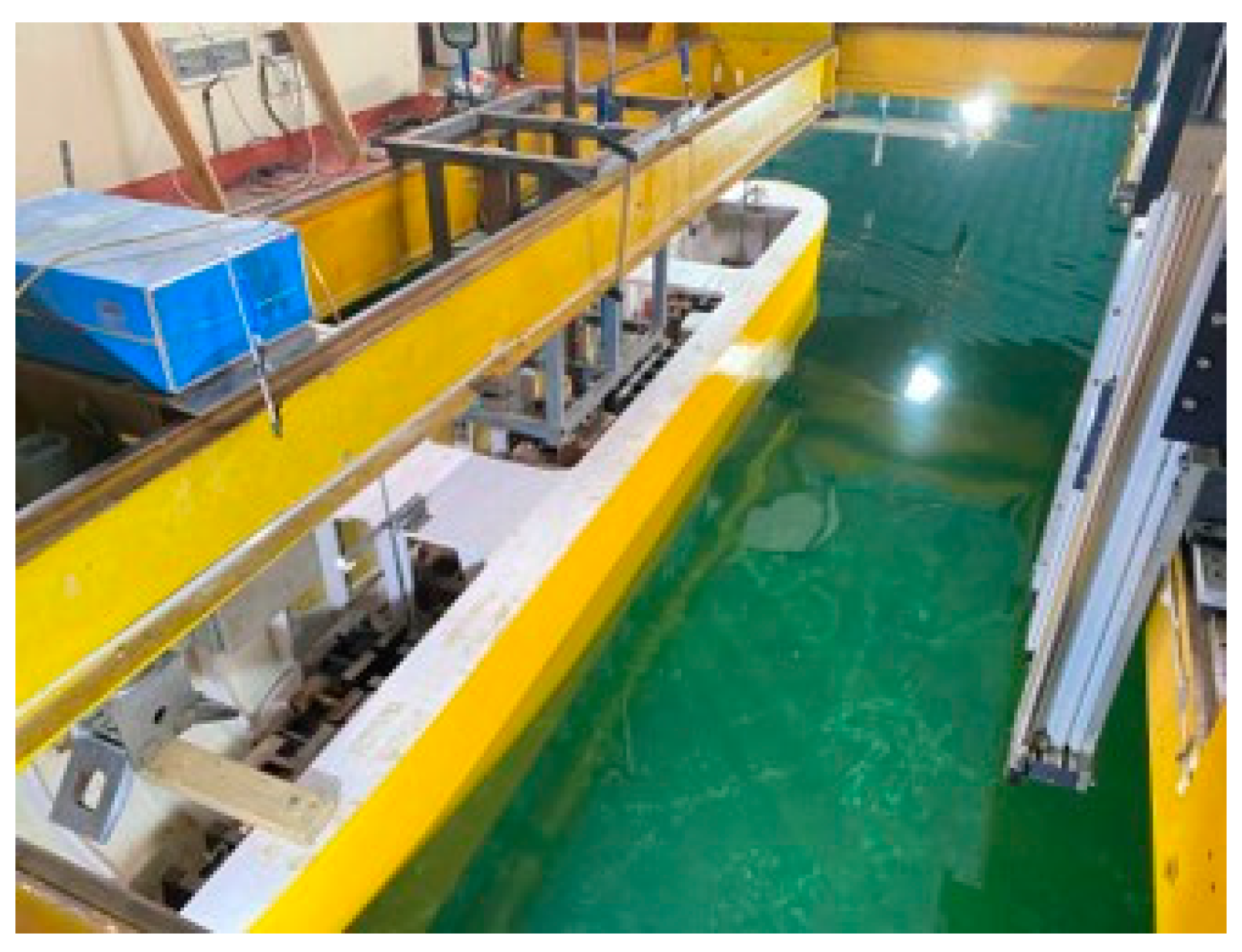
The resistance test was conducted using a small-scale model in accordance with the ITTC regulations at the Ship Model Towing Tank Laboratory of Harbin Engineering University (Figure 2). The test conditions are shown in

Table 2. Conditions of large-scale model test.

Fr	Ship Speed
	Full-Scale (kn)	Small-Scale (m/s)
0.101	11	0.776
0.110	12	0.846
0.119	13	0.917
0.129	14	0.987
0.139	15	1.058
0.147	16	1.128
0.156	17	1.199

.

2.3. Experimental Plan and Procedure of Large-Scale Model Tests in the Port

Traditional resistance tests are typically conducted in towing tanks, where a towing carriage provides the moving speed, and a dynamometer measures the resistance of the model in the forward direction. Drawing inspiration from towing tank tests, this study proposes an effective solution for conducting resistance tests within a port.

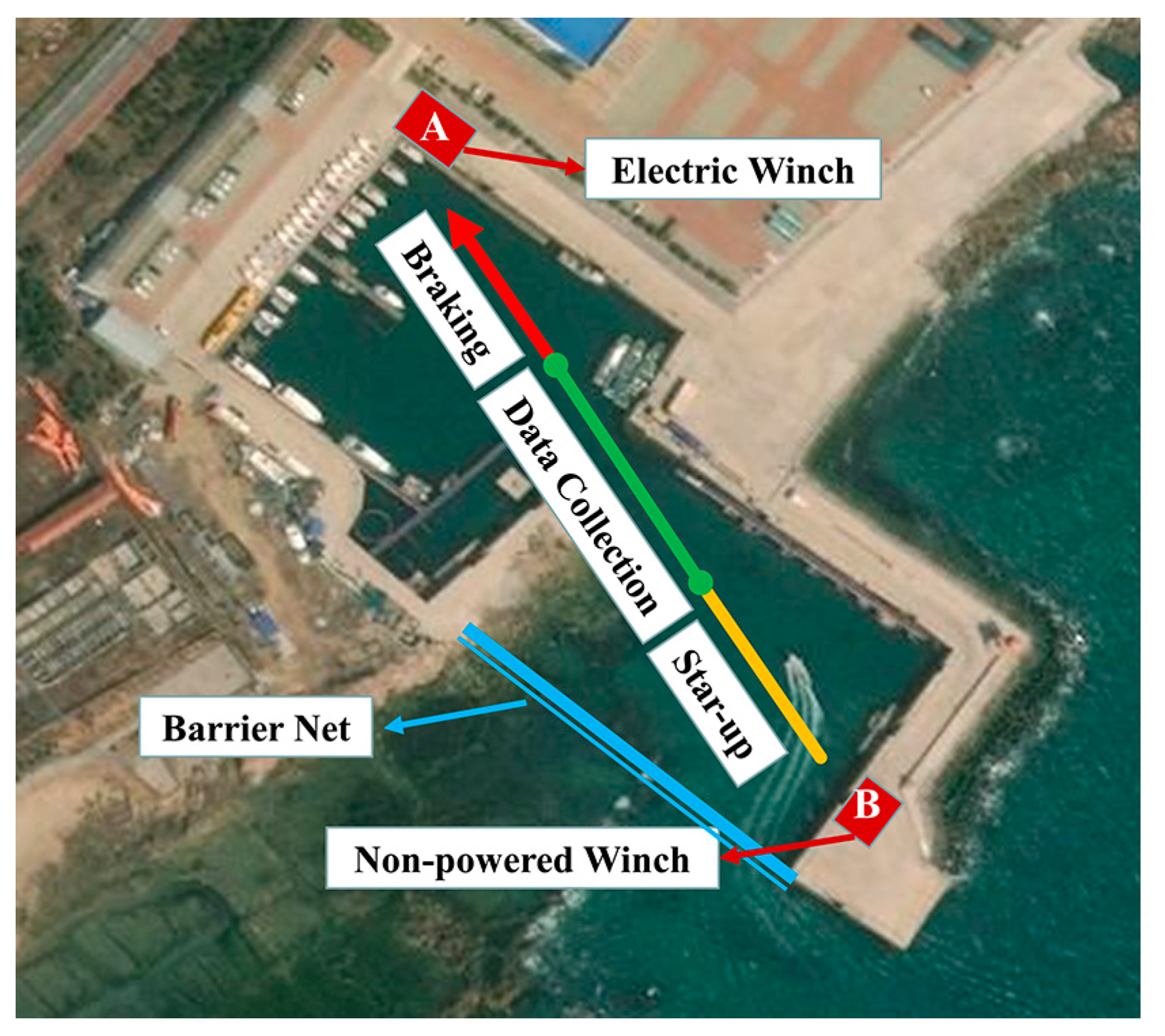
A relatively enclosed harbor basin with high containment (Figure 3) was chosen as the test location. The use of barrier nets helps to block the transmission of small waves from the outside, thus maximizing the simulation of calm water conditions within the harbor. An electric winch is installed at Position A to provide forward towing speed to the model through cable dragging. At Position B, a non-powered winch is used to provide backward tension to the model, limiting any yawing effect. A combination system of Global Positioning System (GPS), Acoustic Doppler Current Profiler (ADCP), and Inertial Navigation System (INS) is utilized to measure the model’s velocity, heading, and other degrees of freedom. Towing points are arranged at the bow and stern columns, and force sensors are connected to the model and cable at these points, using hinge connections. The forces at the two towing points during the model’s forward motion are measured, and the total resistance of the model is calculated through geometric mechanical relationships. The experiment employs a “three-step measurement” method, dividing the entire process into the startup zone, data-collection zone, and braking zone, corresponding to the model’s acceleration, steady motion, and deceleration/stop processes. Data collection for the resistance test is carried out within the data-collection zone.

The low water level, $d$, in the test harbor complies with the requirements for shallow water effects outlined in the ITTC Guidelines 7.5-04-01-01.1:

$$d>2.5T,\mathrm{and}d>2.4V^2/g.$$

(1)

In the equation, T, and V represent the model’s draft, and velocity, respectively; and $g$ represents the acceleration due to gravity (taken as 9.81 m/s²). During the experiment, the wind conditions should ideally not exceed Beaufort Scale 2. Additionally, the experiment is preferably conducted during a period of a relatively calm water surface after the rising tide. During this time, the water flow is slow, and the water level changes minimally within the harbor; this condition is advantageous for the collection and analysis of velocity data.

The complete process of data collection during the experiment generally follows the following steps:

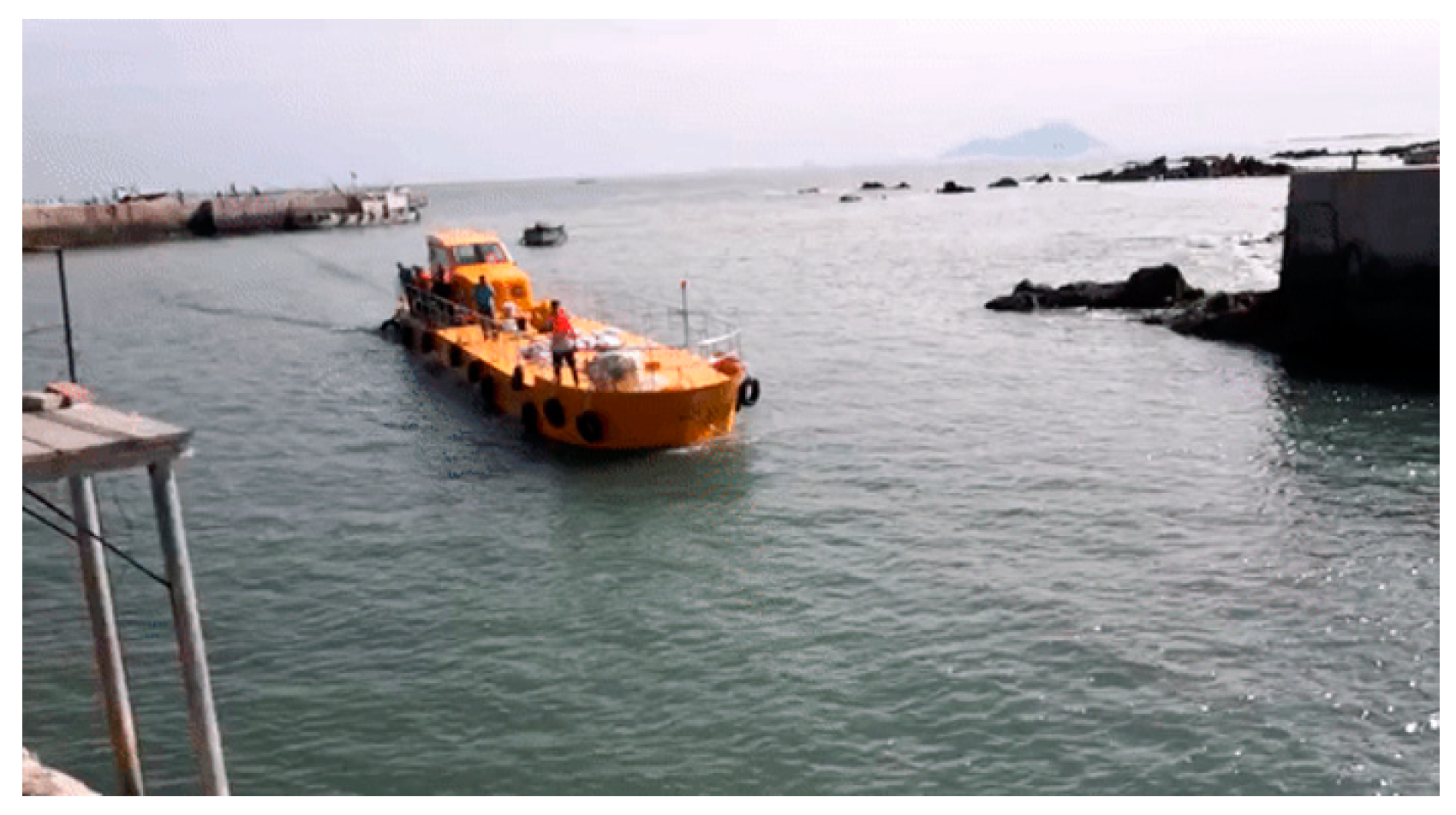
An auxiliary vessel brings the large-scale model to the starting point of the startup zone, in front of the non-powered winch. The bow of the model is aligned as much as possible to face the powered winch, reducing the occurrence of yawing. The powered winch starts rotating at a constant speed, initiating the model’s startup and acceleration. At the same time, the braking system of the non-powered winch is tightened to keep the stern cable taut, assisting in maintaining the heading. This process ensures heading correction. The model then enters the data-collection zone. Inside the deckhouse, the test personnel perform data-collection tasks within this zone (See Figure 4). The collected data include the vessel’s trajectory, speed, bow sensor tension, stern sensor tension, heading angle, average wind speed, average relative wind direction, and the start and end times of data collection (the moment when the bow cable is straightened serves as the initial time). After the data collection is completed, the powered winch is stopped, and the non-powered winch gradually brakes until the model comes to a halt. The auxiliary vessel brings the model back to the starting point of the startup zone to begin the next test.

2.4. Data-Processing Methods for Large-Scale Model Test

2.4.1. Sensor Force Correction

The analysis of resistance characteristics of large-scale models focuses on the water resistance generated in the forward direction of the ship during navigation. However, in experimental testing, the line of action of the measured force by the sensors is not necessarily perpendicular or parallel to the transverse section of the model.

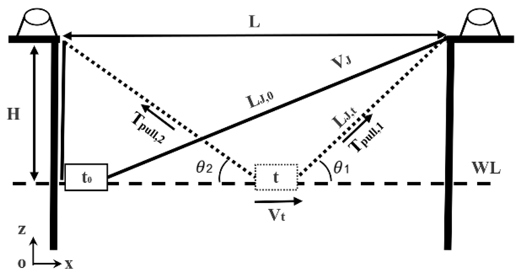
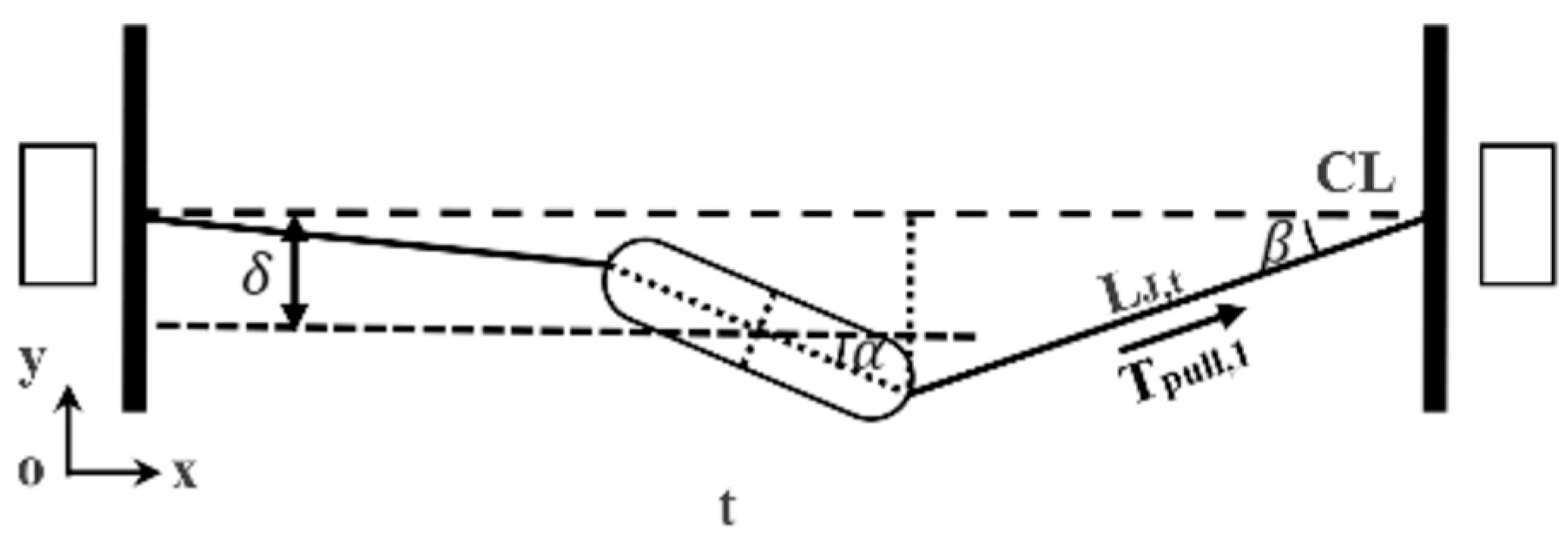
As shown in Figure 5 and Figure 6, there is a difference in elevation (H) between the water surface and the wharf, and the cable has an angle ($\theta$) in the xoz plane; the model is prone to a certain degree of drift ($\delta$) and yaw angle ($\alpha$) during the testing process, and there is another angle ($\beta$) between the cable and the xoy plane. Based on extensive experimental experience, it has been found that the angle ($\theta$) between the cable and the horizontal plane has a significant impact on the analysis of the experimental results. The drift distance ($\delta$) is generally not more than 2 m, and the yaw angle ($\alpha$) does not exceed 2 degrees. When the test interval is sufficiently long, the angle ($\beta$) between the cable and the line connecting to the winch is actually very small, and its influence on the force in the forward direction of the ship can be neglected.

In order to eliminate the influence of the spatial distribution characteristics of the sensor tension on the measurement results, this study mathematically models the magnitude and spatial position of the sensor tension in the xoy plane at any moment during the ship model towing process. The average velocity and average resistance during the data-acquisition period are calculated using an integration averaging method. Prior to the experiment, the distance between the winches ($L$), the water level height difference ($H$), and the total length of the rope at the starting point of the ship model (i.e., at time $t_0$) are measured. At any moment, the relationship satisfied by the tension acting on the ship model is given by the following equation:

$$\begin{array}{l}{L}_{J,t}=L_{J,0}-V_J\times t\\ {\theta }_1=\arcsin \frac{H-H_0}{L_{J,t}}\\ {\theta }_2=\arctan \frac{H-H_0}{L-L_{J,t}\cos {\theta }_1-L_{tw}}\\ V_t=V_J\cos {\theta }_1\\ R_t=T_{pull,1}\cos {\theta }_1-T_{pull,2}\cos {\theta }_2\end{array}\},$$

(2)

where $V_J$ represents the rate of rope retrieval when the winch rotates at a constant speed; $H_0$ denotes the vertical distance between the towing point and the waterline; $L_{J,t}$ represents the length of the rope between the towing point at the bow of the ship model and the winch at time $t$; $L_{tw}$ signifies the distance between the vertical lines through the towing points; ${\theta }_1$ and ${\theta }_2$ represent the angles between the connecting ropes of the towing points at the bow and stern and the horizontal plane, respectively; $T_{pull,1}$ and $T_{pull,2}$ correspond to the magnitudes of the tension at the sensors located at the bow and stern, respectively; $V_t$ denotes the velocity of the ship model; and $R_t$ signifies the magnitude of the resistance acting on the ship model. The average velocity ($\overline{V}$) of the ship model with respect to the ground and the average resistance ($\overline{R}$) during the time interval corresponding to the start and end of data collection at times t₁ and t₂, respectively, can be calculated using the following equation:

$$\begin{array}{l}\overline{V}=\frac{{\displaystyle {\int }_{t_1}^{t_2}{V}_{t}dt}}{t_2-t_1}\\ \overline{R}=\frac{{\displaystyle {\int }_{t_1}^{t_2}{R}_{t}dt}}{t_2-t_1}\end{array}\}.$$

(3)

2.4.2. Wind-Resistance Correction

The large-scale ship model features a deckhouse cabin, and when analyzing the resistance performance of the model, the influence of wind loads on resistance measurement needs to be considered. ITTC 7.5-04-01-01.1 provides specific corrections for the impact of wind loads on ships and proposes CFD numerical simulation methods. Considering the accuracy and cost-effectiveness of the prediction results, this study adopts a CFD numerical method that has been validated with wind-tunnel test data to solve the unsteady Reynolds-averaged Navier–Stokes equations for gas flow and obtain the wind-resistance coefficient.

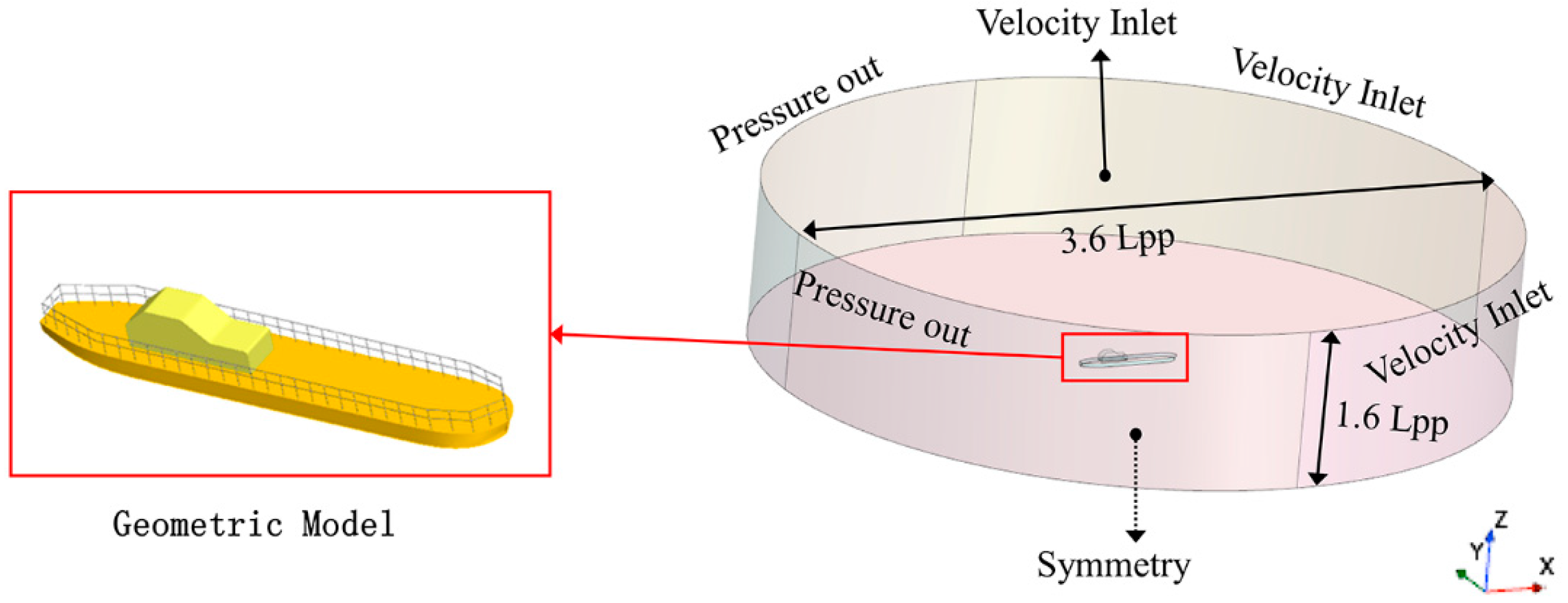
The specific approach is as follows: The governing equations are solved based on pressure. The convective term is discretized using a second-order upwind scheme in spatial discretization. The dissipation term is discretized using a second-order central difference scheme. The SST k-omega turbulence model is employed to close the equations, as it improves the accuracy of simulating adverse pressure gradients by being sensitive to strong flows. The computational model and domain are shown in Figure 7. The lateral sides are set as velocity inlets or pressure outlets based on the incoming flow direction. The top is set as a velocity inlet, the bottom is set as a symmetry plane, and the object surface is set as a no-slip wall. The y+ value on the wall surface is kept below 5. The computational domain is discretized using unstructured polyhedral meshes. The time step is set to 0.01 times the characteristic length divided by the inlet velocity (Δt = 0.01L_PP/V_wind, where V_wind is the inlet velocity, 5 m/s). The geometric model, domain size, and boundary conditions are illustrated in Figure 7. The computational domain takes the form of a cylinder, with the cylindrical surface divided into four equal parts for velocity inlets or pressure outlets (the positions of velocity inlets and pressure outlets are adjusted based on wind direction to avoid additional computational cost due to the rotation angle of the ship model). The top surface is set as a velocity inlet, the bottom surface is set as a symmetry plane, and the ship’s surface is set as a no-slip wall.

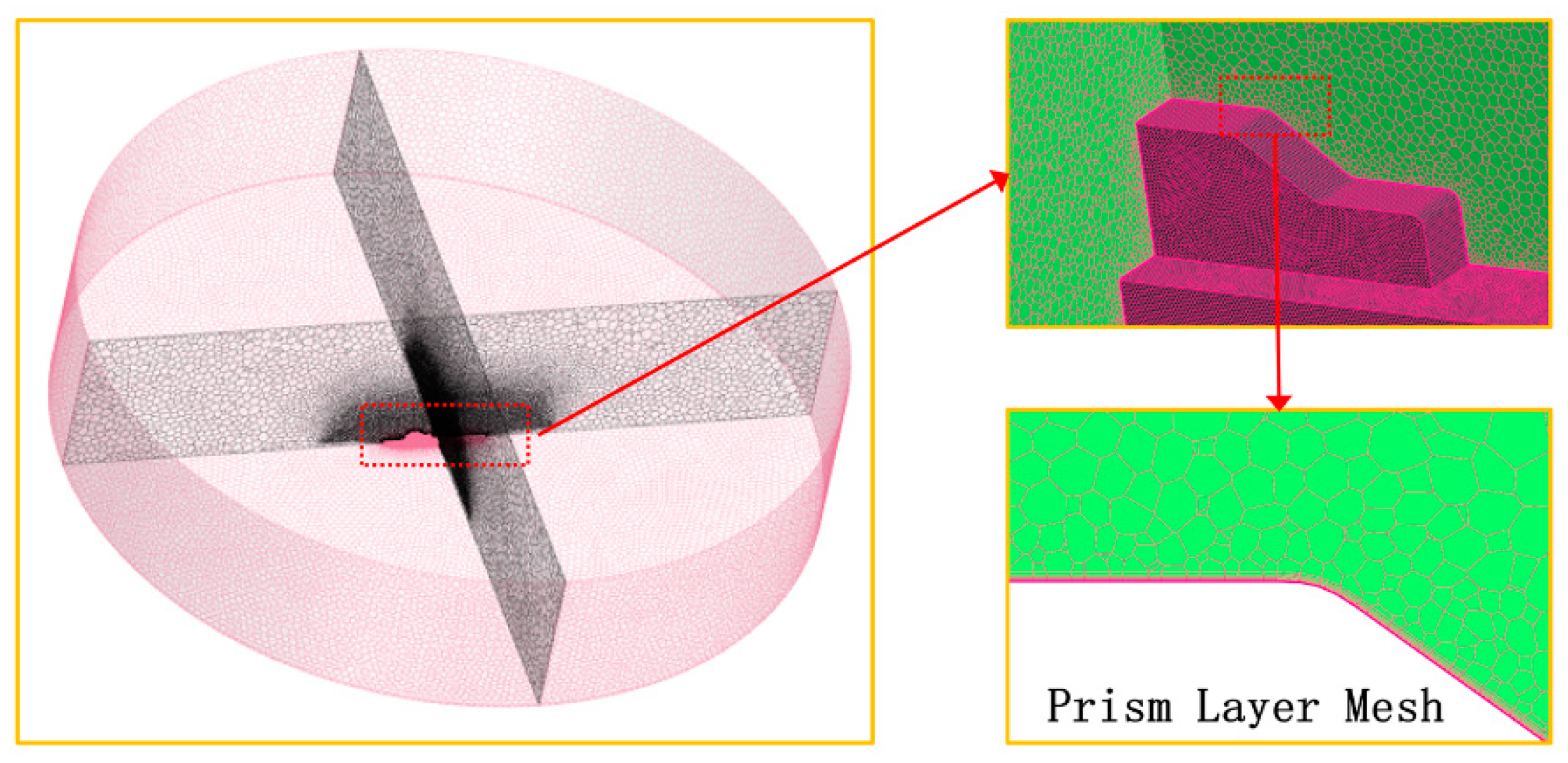
Figure 8 shows the grid topology and details. The grid size on the ship’s surface is 0.05 m, while the grid size near the domain boundaries is 0.8 m. A transition refinement zone (with a basic scale of 0.2 m) is placed near the ship’s body. The total number of grids is approximately 3.7 million.

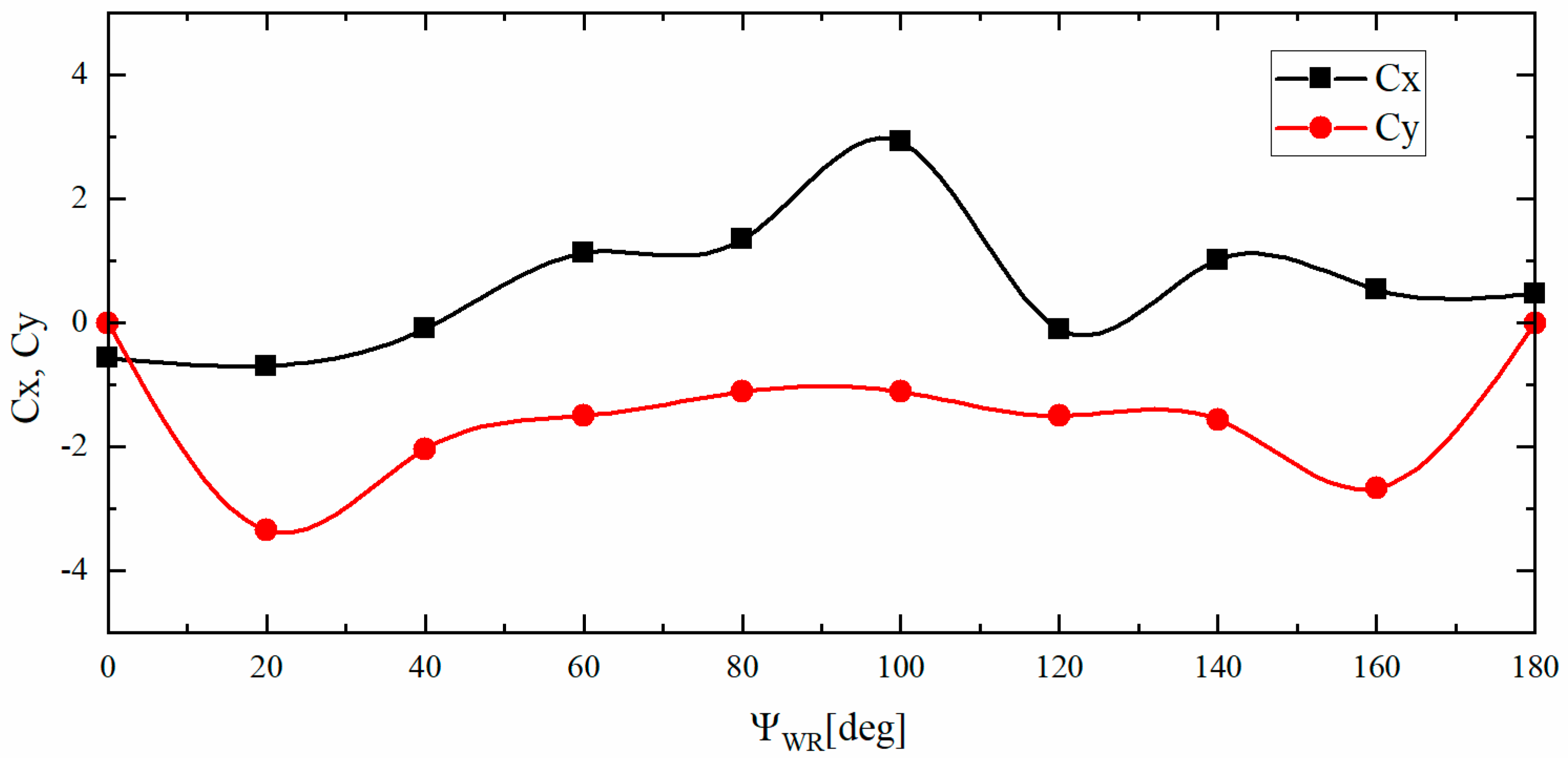
The results of the wind-resistance coefficient calculation are shown in Figure 9. The horizontal axis represents the relative wind direction relative to the bow (0° means head winds) and angles increasing counterclockwise. Cx and Cy represent the dimensionless force coefficients of wind resistance along the ship’s length and width directions, respectively, calculated using Equations (4) and (5):

$$Cx=\frac{F_{wind,x}}{0.5{\rho }_{air}{A}_F{V}_{wind}{}^2},$$

(4)

$$Cy=\frac{F_{wind,y}}{0.5{\rho }_{air}{A}_L{V}_{wind}{}^2}.$$

(5)

In the equation, $F_{wind,x}$ and $F_{wind,y}$ represent the wind resistance along the longitudinal and transverse directions of the ship, respectively; $A_F$ and $A_L$ represent the projected areas of the calculation model on the transverse and longitudinal cross-sections, respectively; ${\rho }_{air}$ denotes the air density; and $V_{wind}$ represents the incoming wind velocity.

The anemometer installed above the driver’s cabin is used to monitor the wind speed and relative wind direction. Based on the average wind direction, interpolation is used to obtain the value of Cy. Then, the wind-resistance correction value is calculated using Equation (4), with the average relative wind speed.

2.4.3. Blockage-Effect Correction

In general, the test basin should be sufficiently large to avoid the influence of blockage and limited water depth. However, due to constraints such as the test site, test environment, and budget limitations, it is difficult to find a perfect test basin. Therefore, when satisfying the requirements for the length and water depth of the test section, it is acceptable to apply blockage correction to sites with certain width limitations. ITTC (2021) provides recommendations for three correction formulas for the blockage effect in resistance tests: Schuster formula, Scott formula, and Tamura formula. Among them, the Scott correction formula is considered to be the best method, as it is suitable for most data. In this study, the width-to-depth ratio at the narrowest point of the test area in the resistance-test basin is approximately 2:1, ranging between 0.08 and 0.16, which meets the conditions for applying the Scott formula. Scott proposed a method to correct the ship model speed for the influence of blockage, as shown in Equation (6):

$$\frac{\Delta V}{V}=K_1\nabla A^{\frac{-3}{2}}+B{L}^2{K}_2{A}^{\frac{-3}{2}},$$

(6)

where $\Delta V$ represents the correction term for the ship speed, $V$ is the ship model speed, $\nabla$ denotes the displacement volume of the ship model, and A represents the cross-sectional area below the water surface at the narrow section. The coefficients $K_1$ and $K_2$ are empirical coefficients, which are calculated using Equations (7) and (8):

$$K_1=\frac{C_B{\nabla }^{\frac{1}{3}}}{Lpp},$$

(7)

$$K_2=\{\begin{array}{l}2.4{(Fr-0.22)}^2,0.22<Fr<0.38\\ 0,else\end{array}.$$

(8)

2.5. Uncertainty Analysis for Large-Scale Model Test

Calculating the uncertainty of error sources in large-scale model tests is a meaningful task. The evaluation process adheres to the GUM (Guide to the Expression of Uncertainty in Measurement) method in the ITTC (2021) 7.5-02-02-02.2 procedure. It analyzes the standard uncertainty, combined uncertainty, and expanded uncertainty of Class B sources. The main sources of uncertainty include the following aspects.

(i) The manufacturing process of the hull cannot guarantee perfect form, which can result in deviations in various principal dimensions. On the other hand, the total ballast quantity remains constant, but variations in actual water temperature can cause changes in the waterline position. These effects are ultimately reflected in the total resistance in terms of the wetted surface area. The estimated deviation in displacement mass is roughly 1 ton, and its uncertainty value can be calculated using Equation (9):

$$u{\prime }_1(R_T)=\frac{2u\prime (\Delta )}{3},$$

(9)

(ii) The measurement errors caused by instrument calibration, such as the force sensor and velocity measurement module, can be replaced with the accuracy values provided by the manufacturer at a 95% confidence interval. The accuracy of each force sensor is 0.02% of the maximum range (with a maximum range of 10 kN), and its uncertainty is calculated according to Equation (10):

$$u{\prime }_2(R_T)=SEE.$$

(10)

The accuracy of the velocity measurement module is 0.02 m/s (at a 95% confidence interval), and the uncertainty is calculated according to Equation (11):

$$u{\prime }_3(R_T)=2u\prime (V).$$

(11)

(iii) The viscosity of seawater affects the Reynolds number and frictional resistance, and its deviation can be obtained from the reading deviation of the thermometer (assuming it follows a uniform distribution). The uncertainty in viscosity is calculated according to Equation (12):

$$u{\prime }_4(R_T)=\left(\frac{C_F}{C_T}\right)\left(\frac{0.87}{Lg\mathrm{Re}-2}\right)u\prime (\upsilon ).$$

(12)

(iv) In Section 2.4, corrections were made for several important influencing factors in the experiments. Many correction formulas involve complex calculations of basic measurement data, such as the distance between winches and the vertical distance between the water level and the winch. The uncertainty of these basic data gradually decreases during the transfer process and can be considered negligible. In Section 2.4.1, the influence of the yaw angle was ignored. In practical testing, the root mean square value of this angle is generally not more than 2 degrees, and we consider that extreme values of drift angle within 5 degrees are acceptable. Assuming that the magnitude of yaw angle remains constant at 5 degrees throughout the entire testing process and that the resulting deviation follows a normal distribution (with a coverage factor equal to 2), the uncertainty of the yaw angle can be calculated using Equation (13).

$$u{\prime }_5(R_T)=\frac{1-\cos \alpha }{2}.$$

(13)

The combined uncertainty of a single measurement is calculated according to Equation (14):

$$u{\prime }_c(R_T)=\sqrt{{(u{\prime }_1)}^2+2{(u{\prime }_2)}^2+{(u{\prime }_3)}^2+{(u{\prime }_4)}^2+2{(u{\prime }_5)}^2}.$$

(14)

Then, the expanded uncertainty (usually with k = 2 for a 95% confidence level) is calculated according to Equation (15):

$$u{\prime }_p(R_T)=k\cdot u{\prime }_c(R_T).$$

(15)

Taking the large-scale resistance test data at a close-to-design speed as an example, the relative uncertainties for various components were calculated, as shown in

Table 3. The results of the uncertainty calculation.

Single Measurement at 15.6 °C: V = 2.089 m/s, RT = 1033.78 N
Components	Symbol	Value (Relative)	Remark
Wetted area	$u{\prime }_1$	0.282%	negligible
Dynamometer	$u{\prime }_2$	0.097%	negligible
Speed	$u{\prime }_3$	0.957%	dominant
Viscosity	$u{\prime }_4$	0.060%	negligible
Yaw angle	$u{\prime }_5$	0.190%	negligible
Combined uncertainty	$u{\prime }_c$	1.044%	Single
Expanded uncertainty	$u{\prime }_p$	2.088%	$k=2$

. The uncertainty of speed is the dominant component, approaching one percent, which is comparable in magnitude to the combined uncertainty. This indicates that the contributions from other sources are negligible and can be disregarded. On the other hand, the value of the expanded uncertainty is approximately 2%, which is well within an acceptable range.

3. Results

3.1. Analysis of Total Resistance

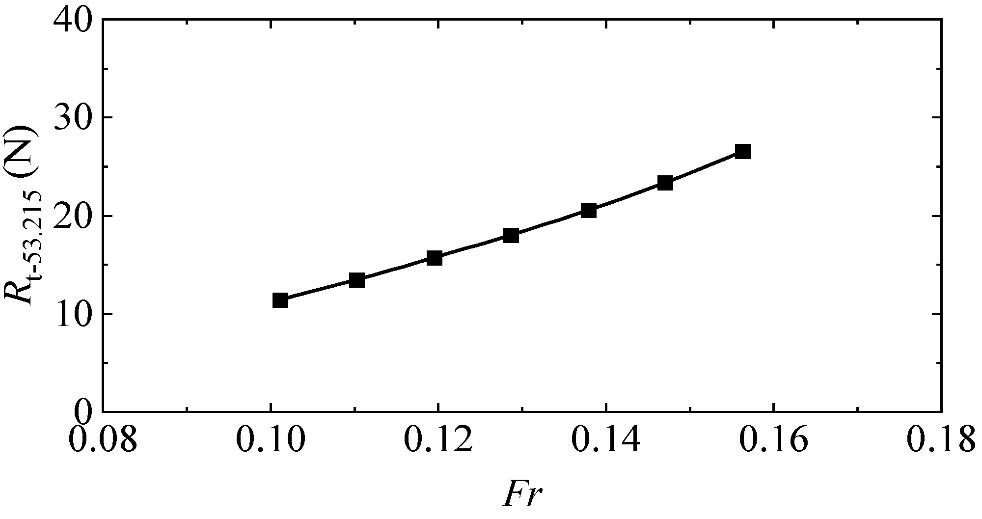
Figure 10 presents the curve showing the variation of total resistance in the towing-tank model resistance test with Froude number. The curve is smooth, and the trend is clear.

The results of the towing tank tests were extrapolated to estimate the resistance values of the large-scale model using both two-dimensional and three-dimensional methods and compared with the actual measured total resistance values of the large-scale model. The two-dimensional method, proposed by Froude, assumes that the ship resistance consists of frictional resistance and residual resistance. It further assumes that the coefficient of residual resistance is only related to the Froude number. In this study, the large-scale model was constructed using fiberglass material with a smooth surface, and the frictional augmentation factor was not considered. Therefore, the extrapolation formula for the two-dimensional method is as follows:

$$C_{ts}=C_{fs}+(C_{tm}-C_{fm}),$$

(16)

where $C_{ts}$ and $C_{tm}$ represent the total resistance coefficients of the ship and model, respectively, while $C_{fs}$ and $C_{fm}$ represent the frictional resistance coefficients of the ship and model, respectively.

The three-dimensional method is also known as the 1 + k method. It assumes that the wave-making resistance coefficient ($C_w$) of the ship is independent of scale effects, and the ratio of viscous pressure resistance coefficient to frictional resistance coefficient is a constant factor (k), known as the form factor. The extrapolation formula for the three-dimensional method is as follows:

$$C_{ts}=C_{tm}+(1+k)(C_{fs}-C_{fm}).$$

(17)

The calculation of the frictional resistance coefficient ($C_f$) is typically performed using the ITTC-1957 empirical formula:

$$C_f=\frac{0.075}{{(\lg Re-2)}^2}.$$

(18)

where Re represents the Reynolds number for both the model ship and the full-scale ship. Grigson made slight adjustments to the ITTC-1957 frictional empirical formula based on actual ship trial data, specifically in the low-Reynolds-number and high-Reynolds-number ranges:

When $Re~(1.5e+6,2e+7)$,

$$C_f=\left[\begin{array}{l}0.93+0.1377{(\lg Re-6.3)}^2\\ -0.06334{(\lg Re-6.3)}^4\end{array}\right]\frac{0.075}{{(LgRe-2)}^2};$$

(19)

When $Re~(1e+8,4e+9)$,

$$C_f=\left[\begin{array}{l}1.032+0.02816{(\lg Re-8)}^2\\ -0.06273{(\lg Re-8)}^4\end{array}\right]\frac{0.075}{{(LgRe-2)}^2};$$

(20)

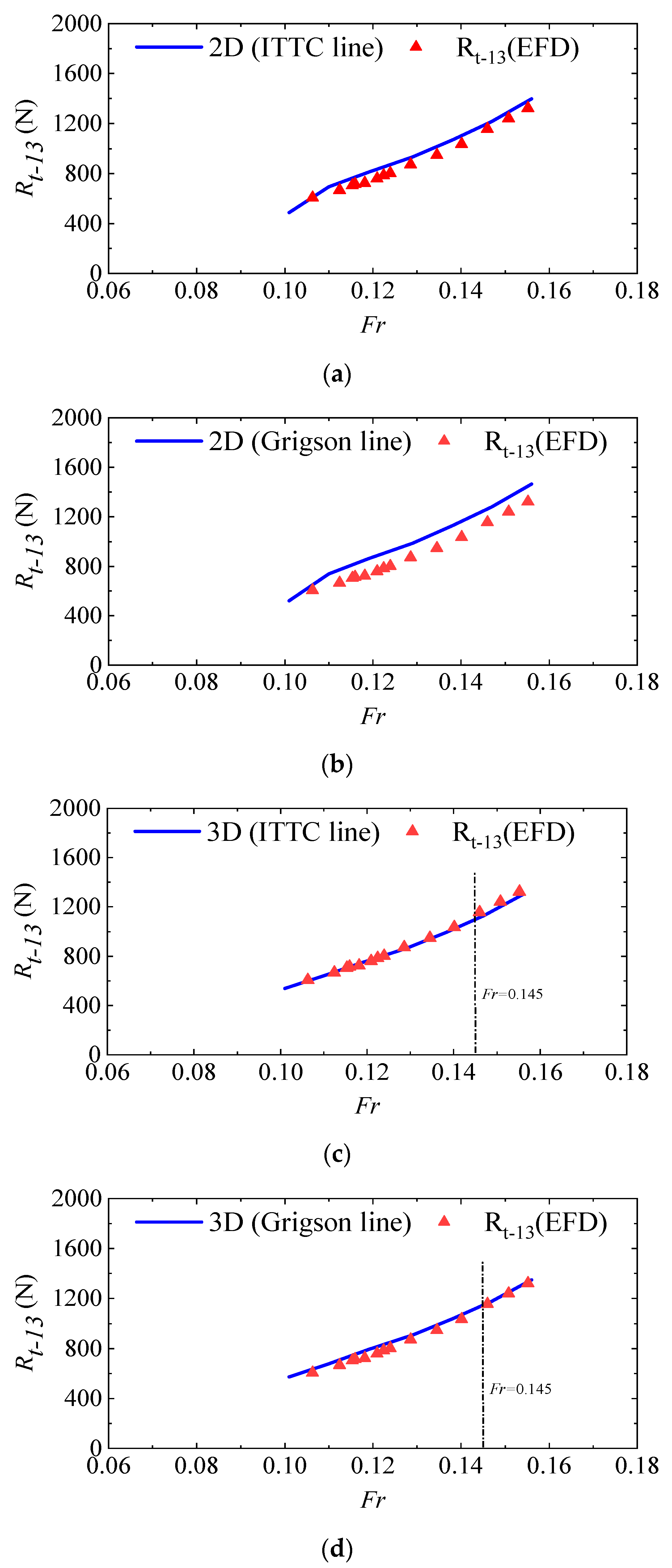
In Figure 11, $R_{t-13}$ represents the total resistance of the large-scale model. Based on the comparative analysis of the extrapolated resistance values from the towing tank model in Figure 11a,b and the measured resistance values of the large-scale model, it can be observed that the 2D method significantly overpredicts the resistance of large-sized vessels. In Figure 11c,d, the predicted resistance values of the large-scale model using the 3D method closely match the experimental results. A further analysis revealed that when the Froude number is less than 0.145, the ITTC empirical formula is more suitable for predicting the frictional resistance. Conversely, when the Froude number is greater than 0.145, the Grigson empirical formula is more applicable. It is recommended to use a mixed format of the ITTC-1957 formula and the Grigson formula, employing the corresponding empirical formula for frictional resistance prediction in different Froude number ranges when analyzing the resistance performance of full-formed vessels.

Based on the ITTC frictional-resistance empirical formula, the form factor of the experimental ship model was determined using Equation (21):

$$C_{tm}/C_{fm}=(1+k)+y\frac{F{r}^4}{C_{fm}}.$$

(21)

The intercept of the fitted line is equal to the value of 1 + k.

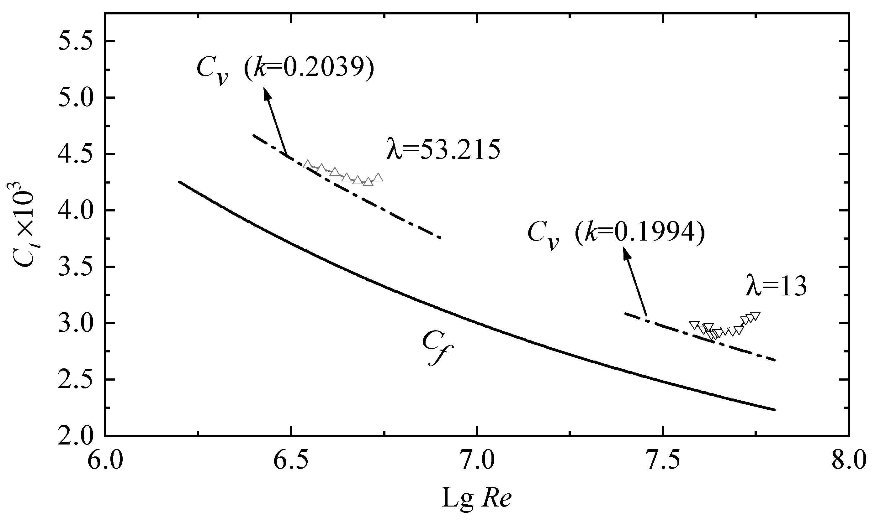
Figure 12 compares the total resistance coefficients and the proportion of viscous pressure components between the two scale models. It can be observed that the form factor (k) for the small-scale model is 0.2039, which is very close to that of the large-scale model. The scale effect is minimal, with a difference of only 2.2%. This also demonstrates the suitability of the three-dimensional method for reasonable extrapolation and conversion of resistance for large-sized vessels.

3.2. Scale Effect of Residual Resistance

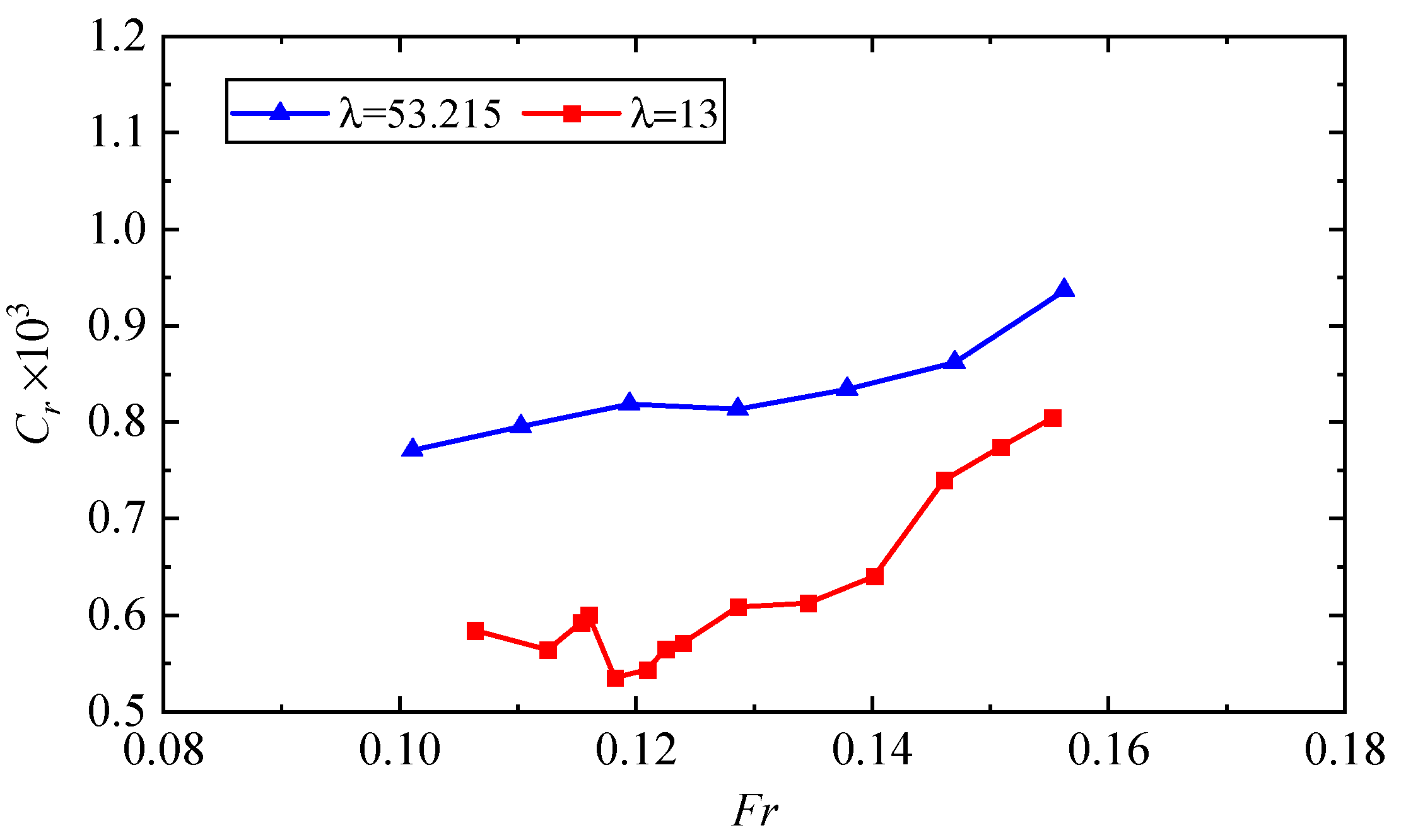
Based on the mixed-format empirical formula for frictional resistance, the residual resistance components of two scale models were compared using the two-dimensional method. Figure 13 provides a clear explanation for the transitional overprediction caused by the two-dimensional method. There is a significant scale effect in the residual resistance components between the two scale models, with the residual resistance coefficient of the small-scale model being much larger than that of the large-scale model.

3.3. Scale Effect of Wave-Making Resistance

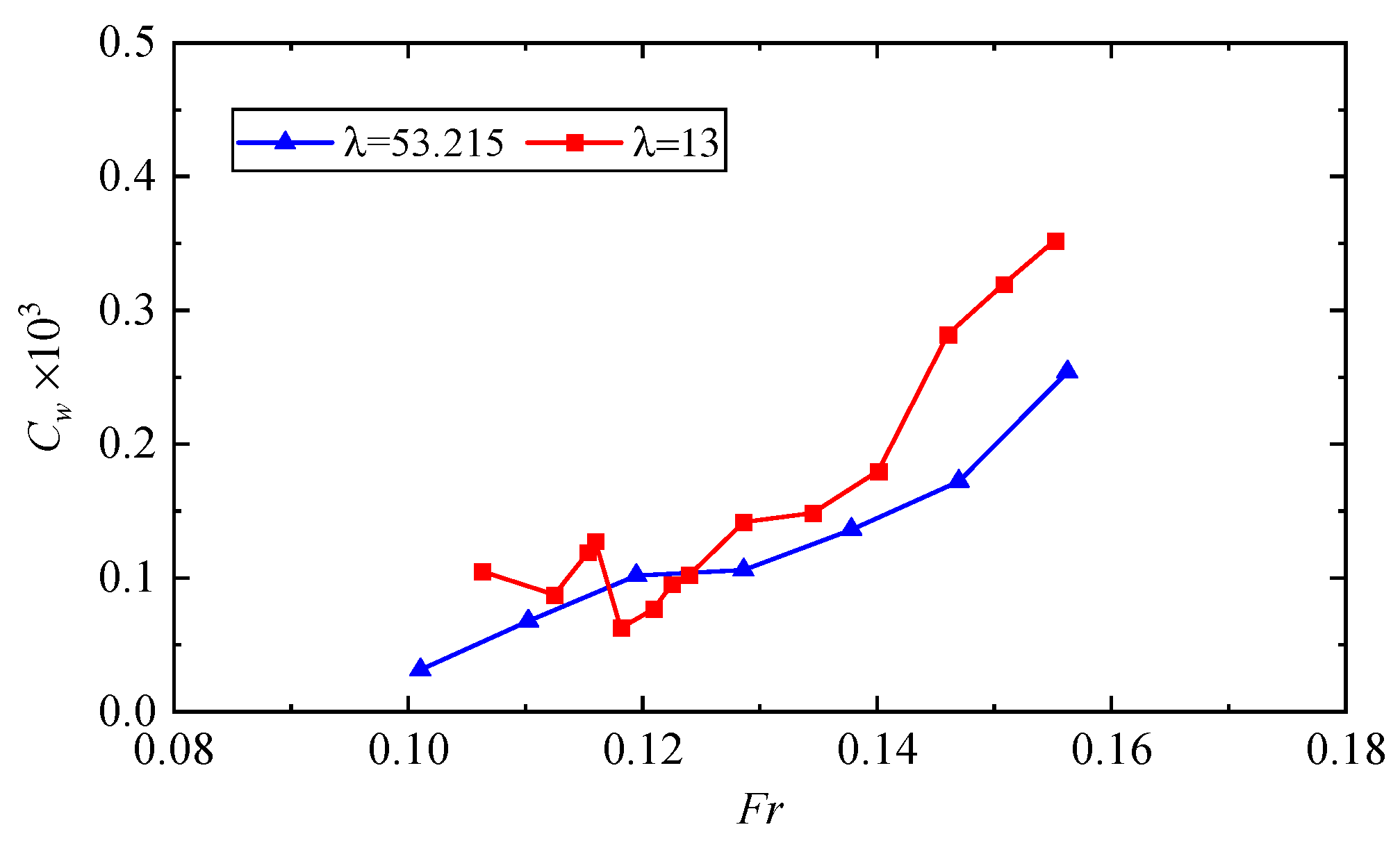
Figure 14 compares the wave-making resistance coefficients of the two scale models when calculating ship frictional resistance based on the ITTC-1957 empirical formula. It can be observed that when the Froude number exceeds 0.125, the wave-making resistance coefficient of the large-scale model is significantly higher than that of the small-scale model, and the difference increases with the increase in the Froude number. Another interesting phenomenon is that when the Froude number is approximately 0.145, the difference suddenly increases, and thereafter, the curves of the wave-making resistance coefficient remain nearly parallel. When the Froude number is greater than 0.145, if the Grigson formula is used to calculate the frictional resistance coefficient, it will increase the proportion of the frictional resistance component, thereby reducing the scale effect of wave-making resistance. Therefore, for Froude numbers greater than 0.145, the Grigson formula is more suitable for predicting the total resistance of large-sized vessels.

4. Conclusions and Discussions

The towing tank imposes limitations on the ship model size, and under the influence of scale effects, the accuracy issue of resistance-performance prediction for large-sized vessels becomes particularly prominent. To overcome the limitations of the testing facility and improve the accuracy of resistance-performance prediction for large-sized vessels, a study was conducted on the resistance-towing test of a 230,000-ton bulk carrier model in a harbor basin. By comparing the results with small-scale model resistance tests in the towing tank, the following conclusions were drawn:

The two-dimensional method significantly overpredicts the resistance of full-formed vessels, while the three-dimensional method provides resistance predictions that are very close to the experimental results. The scale effect on the form factor between the small-scale model in the towing tank and the large-scale model in the harbor basin is minimal, with a difference of only 2.2%. When the Froude number is less than 0.145, the ITTC empirical formula is more suitable for predicting the frictional resistance of full-formed vessels, while the Grigson empirical formula is more suitable when the Froude number is greater than 0.145. It is recommended to use a mixed format of ITTC-1957 formula and Grigson formula, applying the corresponding empirical formula for frictional-resistance prediction in different Froude number ranges, to improve the accuracy of resistance-performance prediction for large-sized vessels.

References

1. Kim, J.H.; Choi, J.E.; Choi, B.J.; Chung, S.H.; Seo, H. Development of energy-saving devices for a full slow-speed ship through improving propulsion performance. Ocean Eng. 2015, 7, 390–398. [Google Scholar] [CrossRef] [Green Version]
2. Attah, E.E.; Bucknall, R. An analysis of the energy efficiency of LNG ships powering options using the EEDI. Ocean Eng. 2015, 110, 62–74. [Google Scholar] [CrossRef]
3. Zaccone, R.; Ottaviani, E.; Figari, M.; Altosole, M. Ship voyage optimization for safe and energy-efficient navigation: A dynamic programming approach. Ocean Eng. 2018, 153, 215–224. [Google Scholar] [CrossRef]
4. Wang, L.Z.; Guo, C.Y.; Su, Y.M.; Wu, T.C. A numerical study on the correlation between the evolution of propeller trailing vortex wake and skew of propellers. Ocean Eng. 2018, 10, 212–224. [Google Scholar] [CrossRef]
5. Wang, L.; Guo, C.; Su, Y.; Xu, P.; Wu, T. Numerical analysis of a propeller during heave motion in cavitating flow. Appl. Ocean Res. 2017, 66, 131–145. [Google Scholar]
6. Dogrul, A.; Song, S.; Demirel, Y.K. Scale effect on ship resistance components and form factor. Ocean Eng. 2020, 209, 107428. [Google Scholar] [CrossRef]
7. Song, K.W.; Guo, C.Y.; Gong, J.; Li, P.; Wang, L.Z. Influence of interceptors, stern flaps, and their combinations on the hydrodynamic performance of a deep-vee ship. Ocean Eng. 2018, 170, 306–320. [Google Scholar] [CrossRef]
8. Song, K.W.; Guo, C.Y.; Wang, C.; Sun, C.; Li, P.; Wang, W. Numerical analysis of the effects of stern flaps on ship resistance and propulsion performance. Ocean Eng. 2019, 193, 106621. [Google Scholar] [CrossRef]
9. Zeng, Q.; Hekkenberg, R.; Thill, C.; Hopman, H. Scale effects on the wave-making resistance of ships sailing in shallow water. Ocean Eng. 2020, 212, 107654. [Google Scholar] [CrossRef]
10. Shen, H.L.; Obwogi, E.O.; Su, Y.M. Scale effects for rudder bulb and rudder thrust fin on propulsive efficiency based on computational fluid dynamics. Ocean Eng. 2016, 117, 199–209. [Google Scholar]
11. Kim, M.; Hizir, O.; Turan, O.; Incecik, A. Numerical studies on added resistance and motions of KVLCC2 in head seas for various ship speeds. Ocean Eng. 2017, 140, 466–476. [Google Scholar] [CrossRef] [Green Version]
12. Song, S.; Demirel, Y.K.; Atlar, M. An investigation into the effect of biofouling on the ship hydrodynamic characteristics using CFD. Ocean Eng. 2019, 175, 122–137. [Google Scholar] [CrossRef] [Green Version]
13. Farkas, A.; Degiuli, N.; Marti, I. Assessment of hydrodynamic characteristics of a full-scale ship at different draughts. Ocean Eng. 2018, 156, 135–152. [Google Scholar] [CrossRef]
14. Shivachev, E.; Khorasanchi, M.; Day, S.; Turan, O. Impact of trim on added resistance of KRISO container ship (KCS) in head waves: An experimental and numerical study. Ocean Eng. 2020, 211, 107594. [Google Scholar] [CrossRef]
15. Duan, W.Y.; Tang, S.X.; Chen, J.K. Power and speed prediction of KVLCC2 in head waves based on TEBEM. Ocean Eng. 2022, 249, 110811. [Google Scholar] [CrossRef]
16. Yldz, B.; Sener, B.; Duman, S.; Datla, R. A numerical and experimental study on the outrigger positioning of a trimaran hull in terms of resistance. Ocean Eng. 2020, 198, 106938. [Google Scholar] [CrossRef]
17. Sun, S.; Chang, X.; Guo, C.; Zhang, H.; Wang, C. Numerical investigation of scale effect of nominal wake of four-screw ship. Ocean Eng. 2019, 183, 208–223. [Google Scholar] [CrossRef]
18. Niklas, K.; Pruszko, H. Full-scale CFD simulations for the determination of ship resistance as a rational, alternative method to towing tank experiments. Ocean Eng. 2019, 190, 106435. [Google Scholar] [CrossRef]
19. Song, K.; Guo, C.; Sun, C.; Wang, C.; Gong, J.; Li, P.; Wang, L. Simulation strategy of the full-scale ship resistance and propulsion performance. Eng. Appl. Comp. Fluid Mech. 2021, 15, 1321–1342. [Google Scholar] [CrossRef]
20. Jiao, J.; Ren, H.; Sun, S.; Liu, N.; Li, H.; Adenya, C.A. A state-of-the-art large scale model testing technique for ship hydrodynamics at sea. Ocean Eng. 2016, 123, 174–190. [Google Scholar] [CrossRef]
21. Jiao, J.; Sun, S.; Li, J.; Adenya, C.A.; Ren, H.; Chen, C.; Wang, D. A comprehensive study on the seakeeping performance of high speed hybrid ships by 2.5D theoretical calculation and different scaled model experiments. Ocean Eng. 2018, 160, 197–223. [Google Scholar] [CrossRef]
22. Jiao, J.; Ren, H.; Soares, C.G. A review of large-scale model at-sea measurements for ship hydrodynamics and structural loads. Ocean Eng. 2021, 227, 108863. [Google Scholar] [CrossRef]
23. Grogan, G.R.; Borthen, J.L. Performing Detailed Design Reviews of a US Navy Surface Combatant within an Integrated Data Environment. J. Ship. Pro. 2010, 26, 66–75. [Google Scholar] [CrossRef]
24. Grigoropoulos, G.J.; Politis, C.G. A Measuring System of the six Degrees of Motions of a Moving Body. J. Ship. Tech. Res. 1999, 45, 4–7. [Google Scholar]
25. Coraddu, A.; Dubbioso, G.; Mauro, S.; Viviani, M. Analysis of twin screw ships’ asymmetric propeller behaviour by means of free running model tests. Ocean Eng. 2013, 68, 47–64. [Google Scholar] [CrossRef] [Green Version]
26. Guo, C.Y.; Zhong, X.H.; Zhao, D.G.; Wang, C.; Lin, J.F.; Song, K.W. Propulsion performance of large-scale ship model in real sea environment. Ocean Eng. 2020, 210, 107440. [Google Scholar] [CrossRef]
27. Su, Y.; Lin, J.; Zhao, D.; Guo, C.; Wang, C.; Guo, H. Real-time prediction of large-scale ship model vertical acceleration based on recurrent neural network. J. Mar. Sci. Eng. 2020, 8, 777. [Google Scholar] [CrossRef]
28. Su, Y.-m.; Lin, J.-f.; Zhao, D.-g.; Guo, C.-y.; Guo, H. Influence of a pre-swirl stator and rudder bulb system on the propulsion performance of a large-scale ship model. Ocean Eng. 2020, 218, 108189. [Google Scholar] [CrossRef]
29. Lin, J.F.; Zhao, D.G.; Guo, C.Y.; Su, Y.M.; Zhong, X.H. Comprehensive test system for ship-model resistance and propulsion performance in actual seas. Ocean Eng. 2020, 197, 106915. [Google Scholar] [CrossRef]
30. Zhou, G.; Wang, Y.; Zhao, D.; Lin, J. Engineering. Uncertainty analysis of ship model propulsion test on actual seas based on Monte Carlo method. J. Mar. Sci. Eng. 2020, 8, 398. [Google Scholar] [CrossRef]
Figure 1. Geometric models: (a) small-scale model and (b) large-scale model.
Jmse 11 01300 g001
Figure 2. Resistance tests in towing tank.
Jmse 11 01300 g002
Figure 3. Resistance tests in towing tank.
Jmse 11 01300 g003
Figure 4. Test scenario.
Jmse 11 01300 g004
Figure 5. Profile projection.
Jmse 11 01300 g005
Figure 6. Horizontal projection.
Jmse 11 01300 g006
Figure 7. Computing domain and boundary conditions.
Jmse 11 01300 g007
Figure 8. Meshes of the computing domain.
Jmse 11 01300 g008
Figure 9. Wind-resistance coefficient.
Jmse 11 01300 g009
Figure 10. Small-scale model resistance curve.
Jmse 11 01300 g010
Figure 11. Comparison between predicted and experimental values of large-scale model resistance: (a) 2D method and ITTC line, (b) 2D method and Grigson line, (c) 3D method and ITTC line, and (d) 3D method and Grigson line.
Jmse 11 01300 g011
Figure 12. Comparison of total resistance coefficients and form factor.
Jmse 11 01300 g012
Figure 13. Comparison of residual resistance coefficients.
Jmse 11 01300 g013
Figure 14. Comparison of wave-making resistance coefficients.
Jmse 11 01300 g014