
Fatigue Analysis of Inter-Array Power Cables between Two Floating Offshore Wind Turbines Including a Simplified Method to Estimate Stress Factors


Abstract
1. Introduction
2. Methodology and Numerical Setup
2.1. Numerical Tools
2.2. Numerical Models
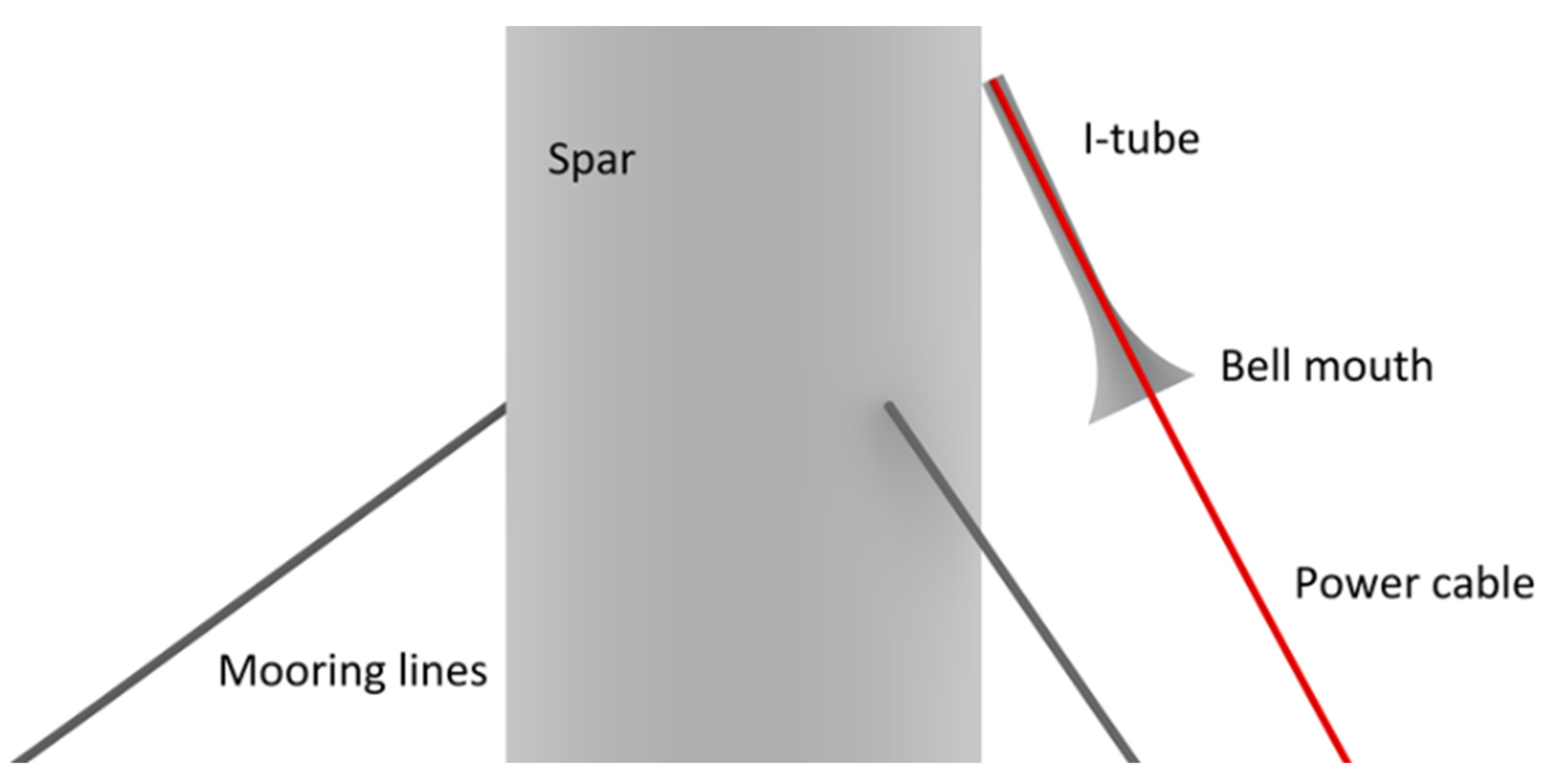
2.2.1. Floating Offshore Wind Turbine System
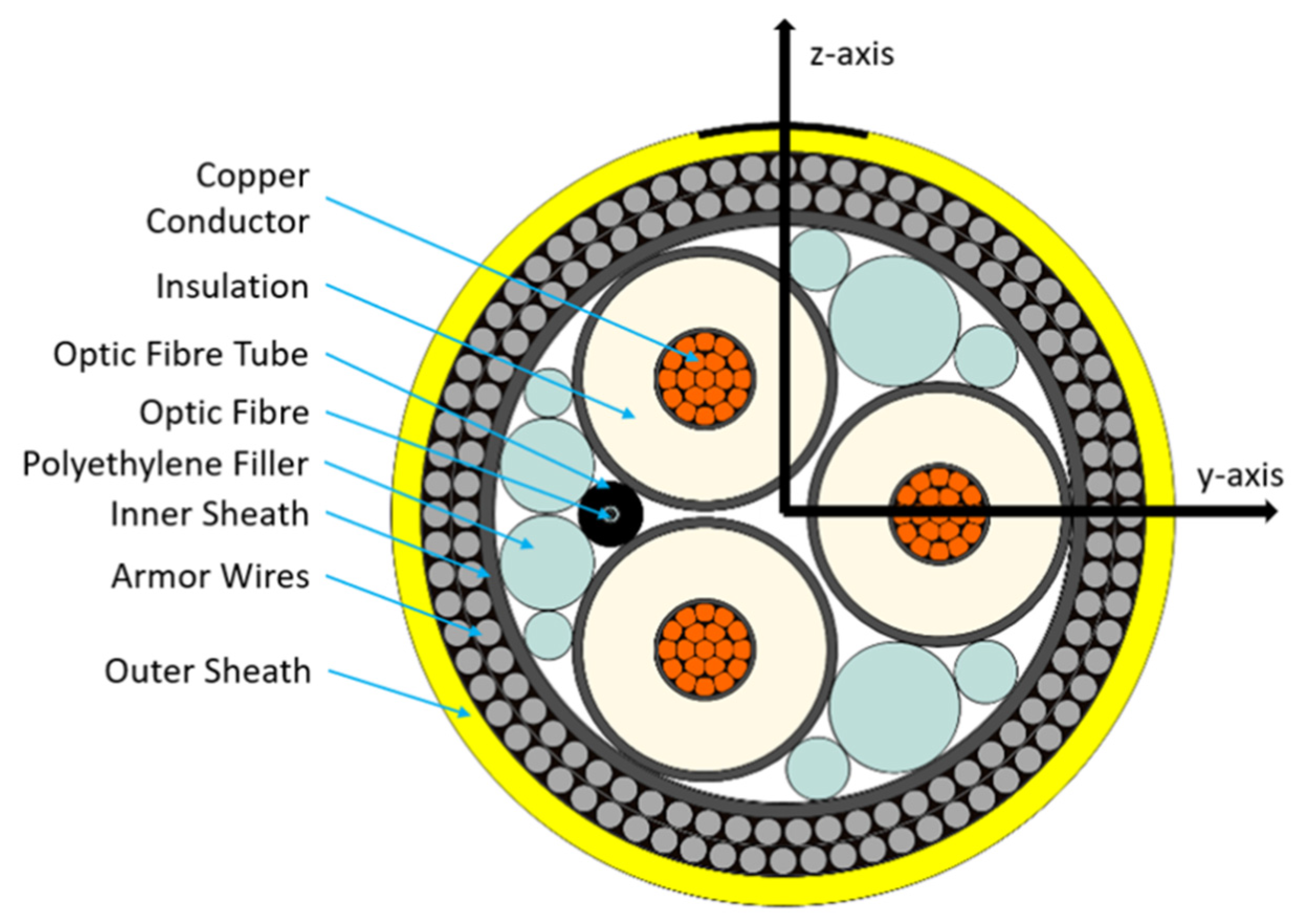
2.2.2. Power Cable Properties
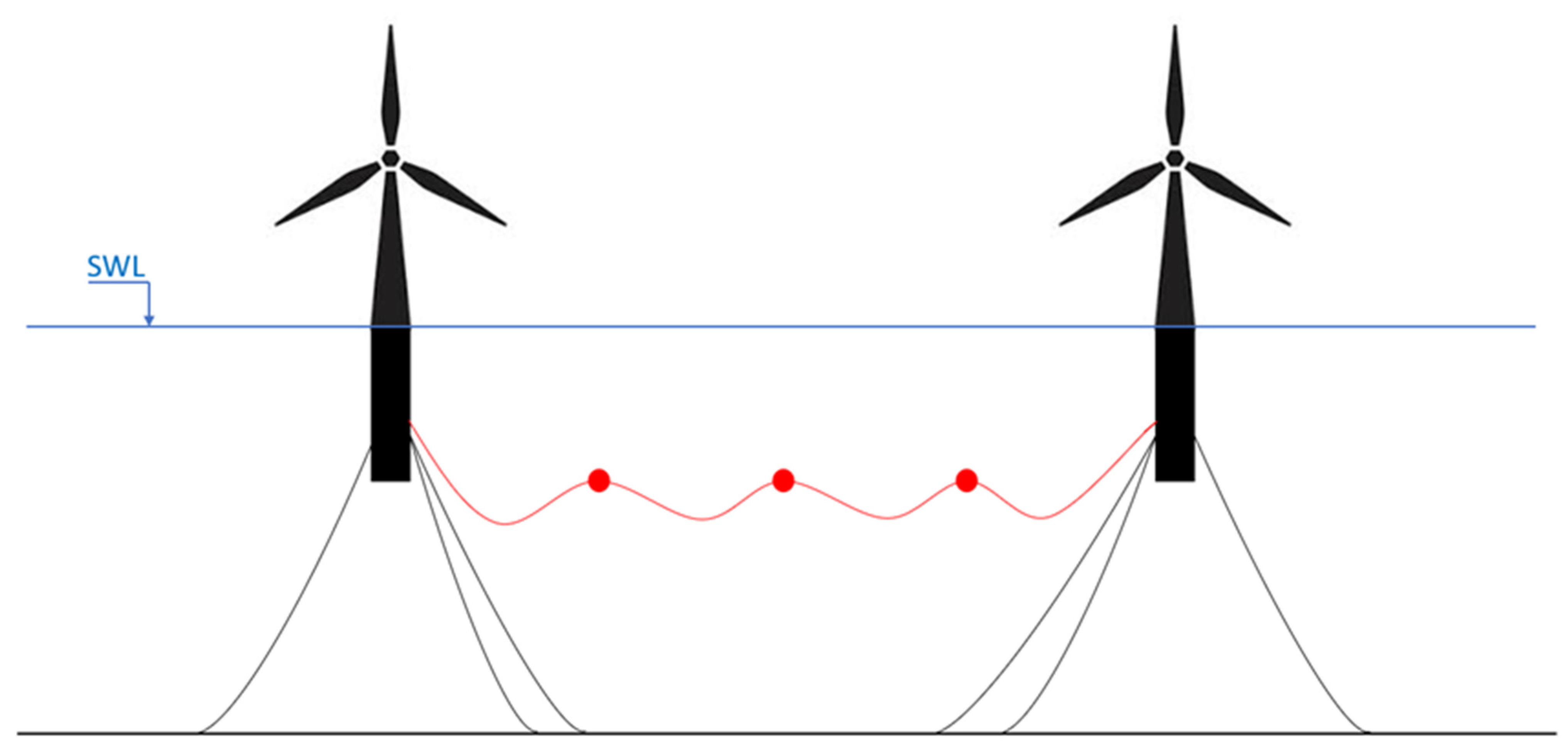
2.2.3. Suspended Power Cable Setup
2.3. Environmental Conditions
2.4. Fatigue Assessment
2.4.1. Nonlinear Bending Behavior Estimation
2.4.2. Calculation of Stresses Using Stress Factors
2.4.3. Dynamic and Fatigue Damage Analysis
3. Results and Discussion
3.1. Nonlinear Bending Behavior
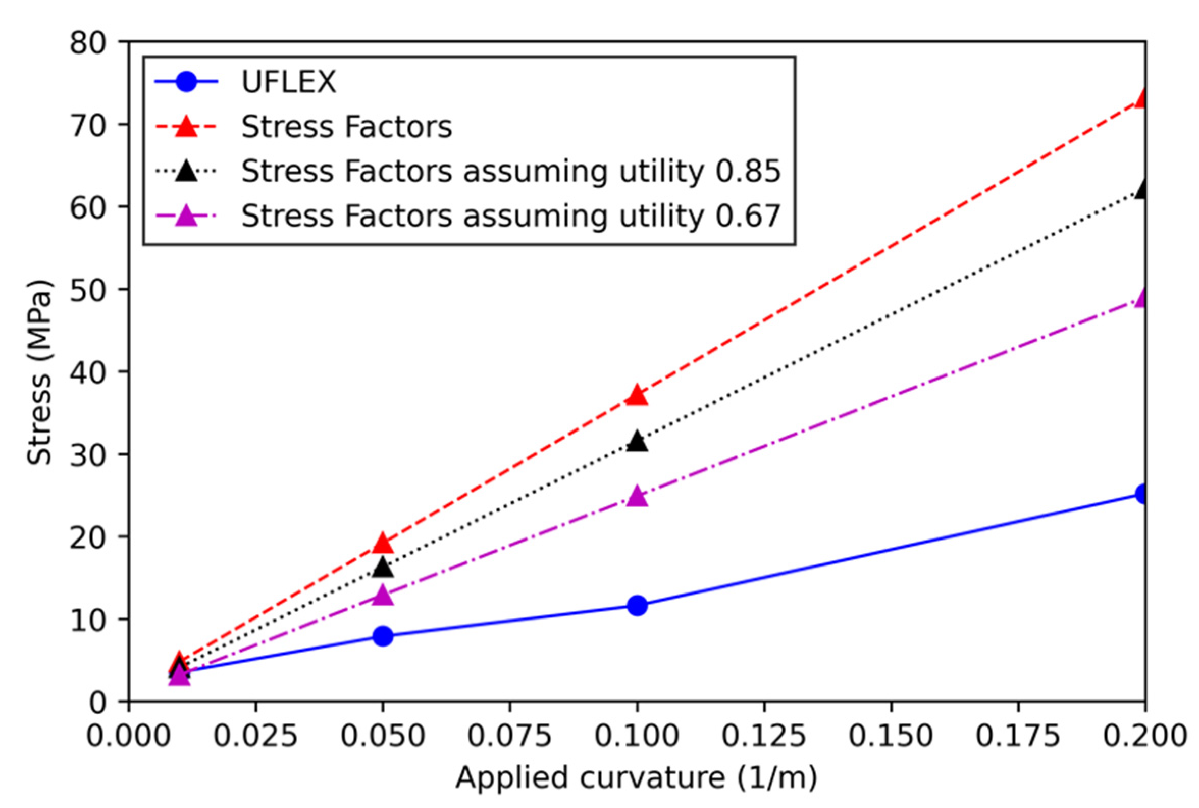
3.2. Results Obtained by the Stress Factor Calculation Methods
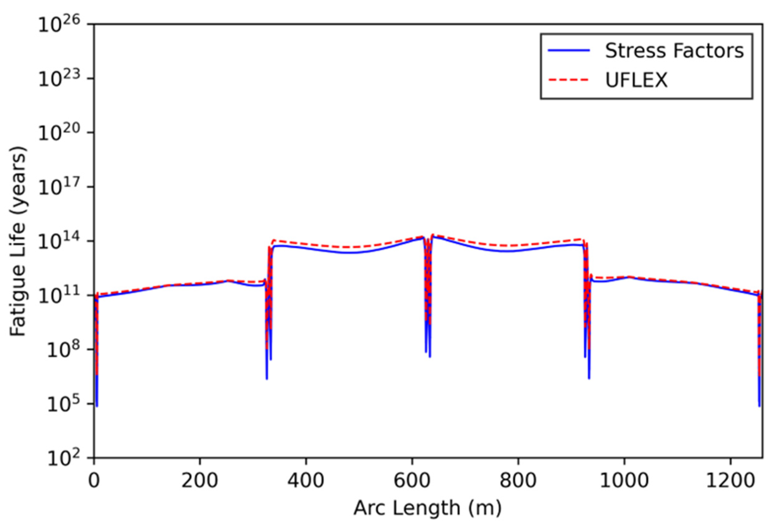
3.3. Fatigue Analysis Results
4. Conclusions
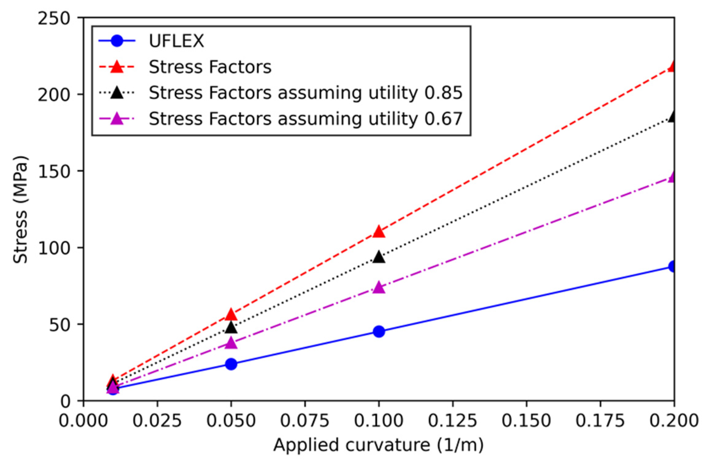
- The proposed stress factor calculation method delivers good results for the selected cable when only tension is applied, based on the comparison with the results from the established finite-element software.
- The proposed stress factor calculation method delivers conservative results when curvature is applied in addition to tension.
- The proposed stress factor estimation method gives conservative results for the preliminary design of the power cable before more reasonable stress factors are known. The fatigue life should be calculated again after the stress factors are obtained through finite element software or experiments.
- The suspended inter-array power cable in the presented configuration has a very long fatigue life resulting from low cyclic loadings.
- The critical areas with respect to fatigue damage are located next to the hang-off points and the buoys. Bending is identified as the main contributor to fatigue damage.
- The estimated fatigue life of the power cable is dependent on the cable and buoy properties. Therefore, the fatigue life should be calculated for each power cable configuration individually.
- The effects of marine growth on the power cable fatigue life are small because large parts of the power cable are located in depths where no marine growth occurs.
Author Contributions
Funding
Institutional Review Board Statement
Informed Consent Statement
Data Availability Statement
Acknowledgments
Conflicts of Interest
References
- Lee, J.; Zhao, F. GWEC-Global-Wind-Report. 2022. Available online: https://gwec.net/wp-content/uploads/2022/03/GWEC-GLOBAL-WIND-REPORT-2022.pdf (accessed on 6 June 2023).
- Cozzi, L.; Wanner, B.; Donovan, C.; Toril, A.; Yu, W. Offshore Wind Outlook 2019: World Energy Outlook Special Report. 2019. Available online: https://iea.blob.core.windows.net/assets/495ab264-4ddf-4b68-b9c0-514295ff40a7/Offshore_Wind_Outlook_2019.pdf (accessed on 6 June 2023).
- Eldøy, S. Hywind Scotland Pilot Park Project Plan for Construction Activities. 2017. Available online: https://marine.gov.scot/sites/default/files/00516548.pdf (accessed on 6 June 2023).
- Principle Power Inc. WindFloat Atlantic. Available online: https://www.principlepower.com/projects/windfloat-atlantic (accessed on 17 November 2022).
- Equinor ASA PUD Hywind Tampen. 2019. Available online: https://www.equinor.com/content/dam/statoil/documents/impact-assessment/hywind-tampen/equinor-hywind-tampen-pud-del-II-konsekvensutredning-mars-2019.pdf (accessed on 6 June 2023).
- Rentschler, M.U.T.; Adam, F.; Chainho, P. Design Optimization of Dynamic Inter-Array Cable Systems for Floating Offshore Wind Turbines. Renew. Sustain. Energy Rev. 2019, 111, 622–635. [Google Scholar] [CrossRef]
- Ikhennicheu, U.; Lynch, M.; Doole, S.; Borisade, F.; Wendt, F.; Schwarzkopf, M.-A.; Matha, D.; Vicente, R.D.; Tim, H.; Ramirez, L.; et al. D3.1 Review of the State of the Art of Dynamic Cable System Design; Corewind: Brussels, Belgium, 2020. [Google Scholar]
- Thies, P.R.; Johanning, L.; Smith, G.H. Assessing Mechanical Loading Regimes and Fatigue Life of Marine Power Cables in Marine Energy Applications. Proc. Inst. Mech. Eng. Part O J. Risk Reliab. 2012, 226, 18–32. [Google Scholar] [CrossRef]
- Thies, P.R.; Harrold, M.; Johanning, L.; Grivas, K.; Georgallis, G. Load and Fatigue Evaluation for 66 KV Floating Offshore Wind Submarine Dynamic Power Cable. 2019. Available online: https://ore.exeter.ac.uk/repository/bitstream/handle/10871/40728/Thies_et%20al_JICABLE2019.pdf?sequence=1&isAllowed=y (accessed on 6 June 2023).
- Bakken, K. Fatigue of Dynamic Power Cables Applied in Offshore Wind Farms. Master’s Thesis, NTNU, Trondheim, Norway, 2019. [Google Scholar]
- Hu, H.; Yan, J.; Sævik, S.; Ye, N.; Lu, Q.; Bu, Y. Nonlinear Bending Behavior of a Multilayer Copper Conductor in a Dynamic Power Cable. Ocean. Eng. 2022, 250, 110831. [Google Scholar] [CrossRef]
- Svensson, G. Fatigue Prediction Models of Dynamic Power Cables by Laboratory Testing and FE Analysis. Master’s Thesis, NTNU, Trondheim, Norway, 2020. [Google Scholar]
- Zhao, S.; Cheng, Y.; Chen, P.; Nie, Y.; Fan, K. A Comparison of Two Dynamic Power Cable Configurations for a Floating Offshore Wind Turbine in Shallow Water. AIP Adv. 2021, 11, 39221. [Google Scholar] [CrossRef]
- Ballard, B.; Yu, Y.-H.; Rij, J.V.; Driscoll, F. Umbilical Fatigue Analysis for a Wave Energy Converter. In Proceedings of the ASME 2020 39th International Conference on Ocean, Offshore and Arctic Engineering, Online, 3–7 August 2020. [Google Scholar]
- Karlsen, S.; Slora, R.; Heide, K.; Lund, S.; Eggertsen, F.; Osborg, P.A. Dynamic Deep Water Power Cables. RAO/CIS OFFSHORE. 2009. Available online: https://books-fmf.clan.su/_ld/1/101_DYNAMICDEEPWATE.pdf (accessed on 6 June 2023).
- Marta, M.; Mueller-Schuetze, S.; Ottersberg, H.; Feu, I.D.; Johanning, L.; Thies, P.R. Development of Dynamic Submarine MV Power Cable Design Solutions for Floating Offshore Renewable Energy Applications. 2015. Available online: https://ore.exeter.ac.uk/repository/bitstream/handle/10871/18314/JICABLE15_0144_final.pdf?sequence=1&isAllowed=y (accessed on 6 June 2023).
- Nasution, F.P.; Sævik, S.; Gjøsteen, J.K.Ø. Fatigue Analysis of Copper Conductor for Offshore Wind Turbines by Experimental and FE Method. Energy Procedia 2012, 24, 271–280. [Google Scholar] [CrossRef]
- Nasution, F.P.; Sævik, S.; Gjøsteen, J.K.Ø. Finite Element Analysis of the Fatigue Strength of Copper Power Conductors Exposed to Tension and Bending Loads. Int. J. Fatigue 2014, 59, 114–128. [Google Scholar] [CrossRef]
- Yang, S.-H.; Ringsberg, J.W.; Johnson, E. Parametric Study of the Dynamic Motions and Mechanical Characteristics of Power Cables for Wave Energy Converters. J. Mar. Sci. Technol. 2018, 23, 10–29. [Google Scholar] [CrossRef]
- Rapha, J.I.; Domínguez, J.L. Suspended Cable Model for Layout Optimisation Purposes in Floating Offshore Wind Farms. J. Phys. Conf. Ser. 2021, 2018, 012033. [Google Scholar] [CrossRef]
- Schnepf, A.; Lopez-Pavon, C.; Ong, M.C.; Yin, G.; Johnsen, Ø. Feasibility Study on Suspended Inter-Array Power Cables between Two Spar-Type Offshore Wind Turbines. Ocean. Eng. 2023, 277, 114215. [Google Scholar] [CrossRef]
- Schnepf, A.; Devulder, A.; Johnsen, Ø.; Ong, M.C.; Lopez-Pavon, C. Numerical Investigations on Suspended Power Cable Configurations for Floating Offshore Wind Turbines in Deep Water Powering an FPSO. J. Offshore Mech. Arct. Eng. 2023, 145, 030904. [Google Scholar] [CrossRef]
- Ahmad, I.B.; Schnepf, A.; Ong, M.C. An Optimization Methodology for Suspended Inter-Array Power Cable Configurations between Two Floating Offshore Wind Turbines. Ocean. Eng. 2023, 277, 114406. [Google Scholar] [CrossRef]
- Orcina Ltd. OrcaFlex. Available online: https://www.orcina.com/webhelp/OrcaFlex/ (accessed on 4 April 2023).
- Python Software Foundation. Python v3.10. Available online: https://w.ww.python.org/ (accessed on 17 November 2022).
- SINTEF. Uflex2D Version 2.8 Theory Manual; SINTEF Ocean: Trondheim, Norway, 2018. [Google Scholar]
- Sævik, S.; Bruaseth, S. Theoretical and Experimental Studies of the Axisymmetric Behaviour of Complex Umbilical Cross-Sections. Appl. Ocean. Res. 2005, 27, 97–106. [Google Scholar] [CrossRef]
- Dai, T.; Saevick, S.; Ye, N. Comparison Study of Umbilicals’ Curvature Based on Full Scale Tests and Numerical Models. In Proceedings of the 26th International Ocean and Polar Engineering Conference, Rhodes, Greece, 26 June 2016; p. 6. [Google Scholar]
- Sævik, S.; Gjøsteen, J.K.Ø. Strength Analysis Modelling of Flexible Umbilical Members for Marine Structures. J. Appl. Math. 2012, 2012, 985349. [Google Scholar] [CrossRef]
- SINTEF. UFLEX Software—Fact Sheet. 2017. Available online: https://www.sintef.no/globalassets/sintef-ocean/pdf/uflexfactsheet_2017_des.pdf (accessed on 6 June 2023).
- Jonkman, J.; Butterfield, S.; Musial, W.; Scott, G. Definition of a 5-MW Reference Wind Turbine for Offshore System Development. National Renewable Energy Laboratory; 2009. Available online: https://www.nrel.gov/docs/fy09osti/38060.pdf (accessed on 6 June 2023).
- Jonkman, J. Definition of the Floating System for Phase IV of OC3. National Renewable Energy Laboratory; 2010. Available online: https://www.nrel.gov/docs/fy10osti/47535.pdf (accessed on 6 June 2023).
- Nexans Norway AS Subsea Composite Cable OM1052 2022.
- DNV. GL AS DNVGL-RP-0005 RP-C203: Fatigue Design of Offshore Steel Structures; DNV: Høvik, Norway, 2014. [Google Scholar]
- Standards Norway. NORSOK N-003—Actions and Action Effects; NORSOK Standards: Oslo, Norway, 2007. [Google Scholar]
- DNV. DNV-RP-C205: Environmental Conditions and Environmental Loads; DNV: Høvik, Norway, 2010. [Google Scholar]
- Spyrou, C.; Mitsakou, C.; Kallos, G.; Louka, P.; Vlastou, G. An Improved Limited Area Model for Describing the Dust Cycle in the Atmosphere. J. Geophys. Res. 2010, 115, D17211. [Google Scholar] [CrossRef]
- Komen, G.J.; Cavaleri, L.; Donelan, M.; Hasselmann, K.; Hasselmann, S.; Janssen, P.A.E.M. Dynamics and Modelling of Ocean Waves; Cambridge University Press: Cambridge, MA, USA, 1994. [Google Scholar]
- WAMDI Group. The WAM Model—A Third Generation Ocean Wave Prediction Model. J. Phys. Oceanogr. 1988, 12, 1775–1810. [Google Scholar]
- Papadopoulos, A.; Nickovic, S.; Missirlis, N. The ETA Model Operational Forecasting System and Its Parallel Implementation. Notes Numer. Fluid Mech. 1997, 62, 176–188. [Google Scholar]
- Asplin, L.; Albretsen, J.; Johnsen, I.A.; Sandvik, A.D. The Hydrodynamic Foundation for Salmon Lice Dispersion Modeling along the Norwegian Coast. Ocean. Dyn. 2020, 70, 1151–1167. [Google Scholar] [CrossRef]
- Gramoll, K. Mechanics—Theory. Available online: https://www.ecourses.ou.edu/cgi-bin/ebook.cgi?topic=me&chap_sec=06.1&page=theory (accessed on 18 November 2022).
- ASTM. International Practices for Cycle Counting in Fatigue Analysis; American Petroleum Institute: Washington, DC, USA, 2011. [Google Scholar]
- Kauzlarich, J.J. The Palmgren-Miner Rule Derived. In Tribology Series; Elsevier: Amsterdam, The Netherlands, 1989; Volume 14, pp. 175–179. ISBN 978-0-444-87435-1. [Google Scholar]
- API. API 17J: Specification for Unbonded Flexible Pipe; American Petroleum Institute: Washington, DC, USA, 2008. [Google Scholar]


| Rotor orientation, configuration | - | Upwind, 3 blades |
| Diameter rotor, hub | m | 126, 3 |
| Hub height | m | 90 |
| Platform total draft | m | 120 |
| Number of mooring lines | - | 3 |
| Angle between mooring lines | ° | 120 |
| Water depth | m | 320 |
| Cut-in, rated, cut-out wind speed | m/s | 3, 11.4, 25 |
| Core main material | − | Copper |
| Voltage rating | kV | 66 |
| Outer diameter | m | 0.116 |
| Mass per unit length | kg/m | 25.0 |
| Length | m | 1260 |
| Torsional stiffness | kNm2 | 38.0 |
| Axial stiffness | MN | 362 |
| Tension at conductor yield | kN | 885 |
| Minimum bending radius | m | 1.8 |
| Drag coefficient | − | 1.2 |
| Added mass coefficient | − | 1.0 |
| Material | Density | Young’s Modulus | Poisson’s Ratio |
|---|---|---|---|
| (kg/m3) | (MPa) | (-) | |
| Copper | 8900 | 95,000 | 0.30 |
| Steel | 7800 | 200,000 | 0.30 |
| XLPE | 950 | 800 | 0.45 |
| Marine Growth State | Water Depth | Outer Diameter | Mass per Unit Length |
|---|---|---|---|
| (m) | (m) | (kg/m) | |
| SOL | Below −100 | 0.116 | 25.0 |
| EOL1 | −100 to −60 | 0.156 | 34.4 |
| EOL2 | −60 to −50 | 0.176 | 40.1 |
| Length | m | 2.170 |
| Volume | m3 | 8.615 |
| Mass | kg | 2700 |
| Equivalent buoy outer diameter (cylinder shape) | m | 2.248 |
| Drag coefficient (normal) | − | 0.209 |
| Drag coefficient (axial) | − | 1.000 |
| Added mass coefficient (normal) | − | 0.459 |
| Added mass coefficient (axial) | − | 0.600 |
| Load | Wave Hs | Wave Tp | Current at SWL | Windspeed at Hub Height | Probabilities |
|---|---|---|---|---|---|
| case | (m) | (s) | (m/s) | (m/s) | |
| 1 | 1.2 | 8.3 | 0.06 | 3.7 | 21.0% |
| 2 | 0.9 | 9.9 | 0.12 | 7.5 | 5.09% |
| 3 | 0.9 | 4.0 | 0.12 | 7.5 | 3.33% |
| 4 | 1.9 | 13.5 | 0.12 | 7.5 | 7.56% |
| 5 | 1.9 | 11.7 | 0.12 | 7.5 | 10.56% |
| 6 | 3.0 | 11.8 | 0.15 | 9.4 | 5.80% |
| 7 | 3.0 | 13.6 | 0.15 | 9.4 | 7.08% |
| 8 | 1.0 | 15.0 | 0.15 | 10.4 | 2.39% |
| 9 | 3.8 | 8.0 | 0.17 | 10.4 | 2.50% |
| 10 | 4.5 | 13.4 | 0.18 | 11.4 | 3.84% |
| 11 | 1.9 | 6.4 | 0.18 | 11.4 | 4.12% |
| 12 | 3.7 | 10.0 | 0.18 | 11.4 | 4.10% |
| 13 | 4.0 | 6.3 | 0.2 | 12.9 | 0.90% |
| 14 | 1.8 | 8.2 | 0.2 | 12.9 | 1.60% |
| 15 | 4.0 | 10.1 | 0.2 | 12.9 | 4.09% |
| 16 | 4.0 | 11.6 | 0.2 | 12.9 | 1.66% |
| 17 | 4.0 | 13.2 | 0.2 | 12.9 | 1.07% |
| 18 | 1.3 | 17.1 | 0.2 | 12.9 | 0.43% |
| 19 | 3.3 | 8.1 | 0.24 | 14.9 | 1.97% |
| 20 | 3.9 | 15.3 | 0.24 | 14.9 | 2.99% |
| 21 | 3.9 | 17.0 | 0.24 | 14.9 | 0.16% |
| 22 | 5.9 | 9.1 | 0.28 | 17.7 | 0.84% |
| 23 | 5.9 | 11.4 | 0.28 | 17.7 | 1.43% |
| 24 | 5.9 | 12.0 | 0.28 | 17.7 | 1.37% |
| 25 | 5.9 | 14.9 | 0.28 | 17.7 | 1.33% |
| 26 | 7.4 | 9.8 | 0.35 | 21.5 | 0.22% |
| 27 | 8.5 | 11.5 | 0.35 | 21.5 | 0.81% |
| 28 | 9.0 | 13.7 | 0.35 | 21.5 | 1.53% |
| 29 | 9.0 | 16.0 | 0.35 | 21.5 | 0.10% |
| 30 | 11.9 | 13.8 | 0.47 | 30 | 0.13% |
| Components | Tension Stress Factor, Kt | Curvature Stress Factor, Kc |
|---|---|---|
| (kPa/kN) | (kPa/(1/m)) | |
| Copper wires | 232.3 | 360,000 |
| Armor steel wires | 489.0 | 1,080,000 |
| Components | Tension Stress Factor, Kt | Curvature Stress Factor, Kc |
|---|---|---|
| (kPa/kN) | (kPa/(1/m)) | |
| Copper wires | 232.3 | 150,000 |
| Armor steel wires | 489.0 | 500,000 |
| Specified Loads | Model Including Friction (MPa) | Zero-Friction Model (MPa) | Deviation (Zero-Friction to Friction) | |||
|---|---|---|---|---|---|---|
| Armor | Copper | Armor | Copper | Armor | Copper | |
| 20 kN axial, 0.05 1/m curvature | 31.9 | 12.4 | 31.1 | 10.7 | −2.5% | −13.7% |
| 50 kN axial, 0.1 1/m curvature | 68.2 | 26.7 | 67.1 | 23.9 | −1.6% | −10.5% |
| 50 kN axial, 0.2 1/m curvature | 110.0 | 37.9 | 109.7 | 36.2 | −0.3% | −4.5% |
| Marine Growth State | Minimum Fatigue Life (Years) | Component | Location (m) | Location (Angle) |
|---|---|---|---|---|
| SOL | 71.06 · 103 | Copper Wires | 5.85 | 90° |
| EOL | 65.90 · 103 | Copper Wires | 5.85 | 90° |
Disclaimer/Publisher’s Note: The statements, opinions and data contained in all publications are solely those of the individual author(s) and contributor(s) and not of MDPI and/or the editor(s). MDPI and/or the editor(s) disclaim responsibility for any injury to people or property resulting from any ideas, methods, instructions or products referred to in the content. |
© 2023 by the authors. Licensee MDPI, Basel, Switzerland. This article is an open access article distributed under the terms and conditions of the Creative Commons Attribution (CC BY) license (https://creativecommons.org/licenses/by/4.0/).
Share and Cite
Beier, D.; Schnepf, A.; Van Steel, S.; Ye, N.; Ong, M.C. Fatigue Analysis of Inter-Array Power Cables between Two Floating Offshore Wind Turbines Including a Simplified Method to Estimate Stress Factors. J. Mar. Sci. Eng. 2023, 11, 1254. https://doi.org/10.3390/jmse11061254
Beier D, Schnepf A, Van Steel S, Ye N, Ong MC. Fatigue Analysis of Inter-Array Power Cables between Two Floating Offshore Wind Turbines Including a Simplified Method to Estimate Stress Factors. Journal of Marine Science and Engineering. 2023; 11(6):1254. https://doi.org/10.3390/jmse11061254
Chicago/Turabian StyleBeier, Dennis, Anja Schnepf, Sean Van Steel, Naiquan Ye, and Muk Chen Ong. 2023. "Fatigue Analysis of Inter-Array Power Cables between Two Floating Offshore Wind Turbines Including a Simplified Method to Estimate Stress Factors" Journal of Marine Science and Engineering 11, no. 6: 1254. https://doi.org/10.3390/jmse11061254
APA StyleBeier, D., Schnepf, A., Van Steel, S., Ye, N., & Ong, M. C. (2023). Fatigue Analysis of Inter-Array Power Cables between Two Floating Offshore Wind Turbines Including a Simplified Method to Estimate Stress Factors. Journal of Marine Science and Engineering, 11(6), 1254. https://doi.org/10.3390/jmse11061254