A Ship Route Planning Method under the Sailing Time Constraint
Abstract
1. Introduction
2. Dynamic Sea Environment Model
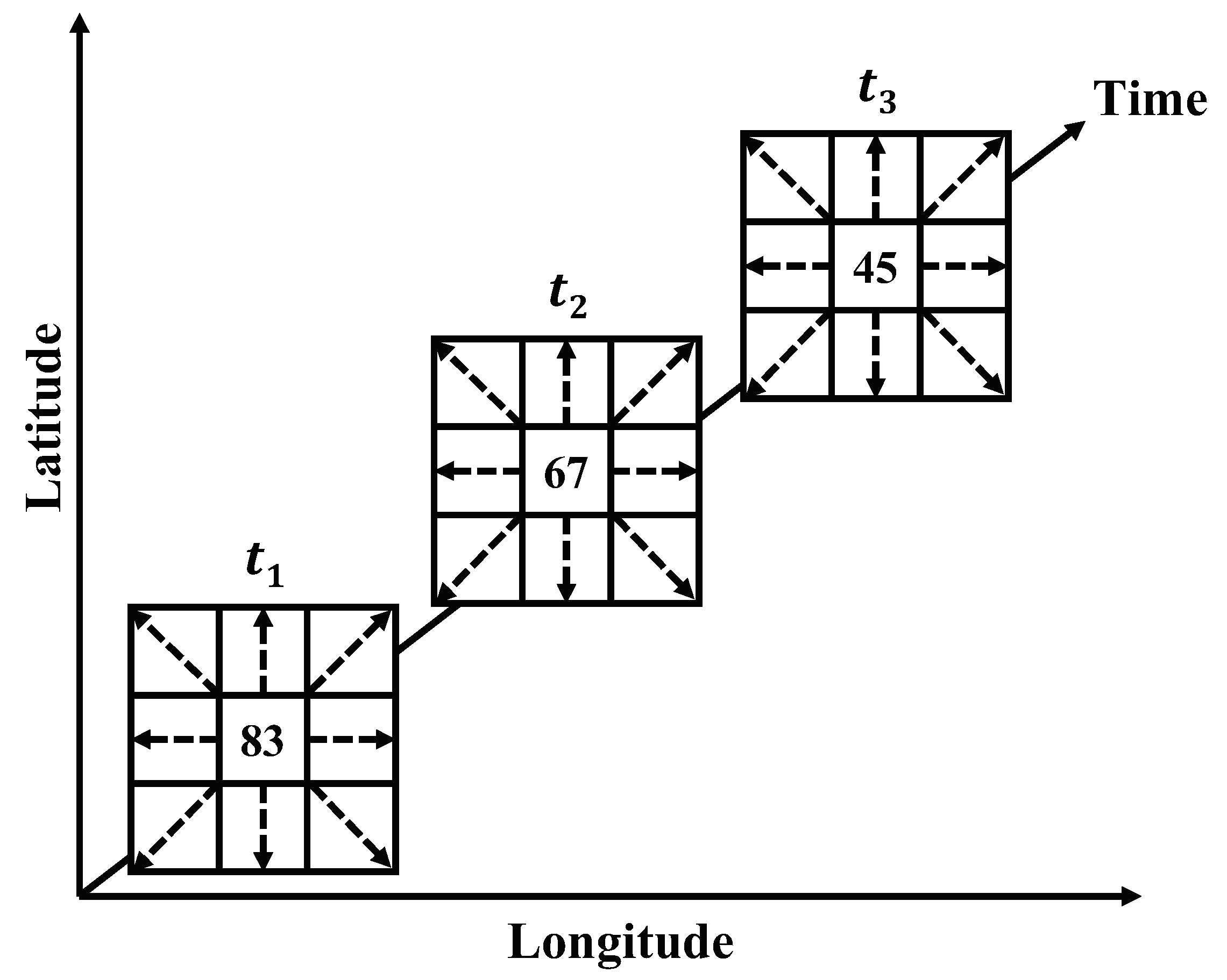
2.1. Three-Dimensional Sea Environment Model
- The ship should navigate in an area with sufficient water depth.
- The ship should not sail in dangerous wind and wave conditions.
- The route plan should consider dynamic meteorological and sea conditions for long-distance and long-term navigation.
2.2. Binarization of Navigation Area
3. Predictive Model for Ship Parameters
3.1. Pre-Processing of Data
- Remove anomalous records in which data are incomplete, such as missing latitude and longitude data.
- To reduce the complexity of the artificial neural network mentioned later, the absolute directions of weather are converted to the directions to the ship reference frame:where represents directions of weather components (wind and wave) to the ship’s reference frame, is the ship’s course, and is the absolute directions of weather components.
- According to this method [40], extract sequential records of approximately 10 min and combine them into one segment.
- Calculate the mean value of each type of data in a segment.For data that are not measured as angles, the mean for the N data points in a segment with values is computed byFor data that are measured as angles, the mean is computed by
- Calculate the standard error of the mean of each type of data in a segment. The standard error of the mean is computed byFor data not measured as angles, the difference is computed byFor data measured as angles, the difference is computed by
- Two thresholds are used to delete segments in which the standard error of the mean of certain data is too large. In particular, if the of RPM is greater than 3 min or the of SOG is greater than 0.5 kt, then all records in that segment are deleted. After this operation, several uniform sailing segments are obtained.
- We use Chauvenet’s criterion to determine if data are anomalous in each uniform sailing segment. Once a data point is identified as an outlier based on the criterion, it is removed. A new mean and standard error of the mean can be calculated based on the remaining values and the new sample size.The probability for the occurrence of any is computed bywhere is the probability of occurrence of and is the complementary error function.A datum is considered an outlier if Formula (10) is fulfilled.This method cleans the original voyages’ records to obtain several navigation segments with a duration of about 10 min and a uniform speed. The mean values of these segments’ data can be used for subsequent training and prediction of the model.
- The different types of input data have different units. It would reduce the performance and convergence of the predictive model if the filtered data of the segments were input into the neural network directly. Therefore, the z-score standardization method is adopted to standardize the data:where is one type of data in a segment after the standardization, is this type of data unprocessed in the segment, and and are the mean and standard error value of this type of data in all segments.
3.2. Predictive Model for Ship Parameters
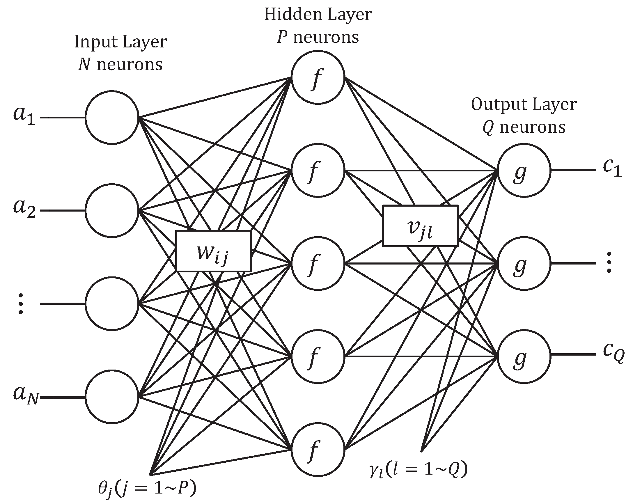
3.2.1. Structure of the Predictive Model
3.2.2. Error Back-Propagation Algorithm
3.3. Selection of Model Variables
- They can represent the current navigation state or navigation environment of the ship.
- They can be obtained or predicted in some way in the route planning process.
- How the data are obtained or predicted cannot be too complex or take up too much running time.
4. Co-Optimization of Ship Course and Speed
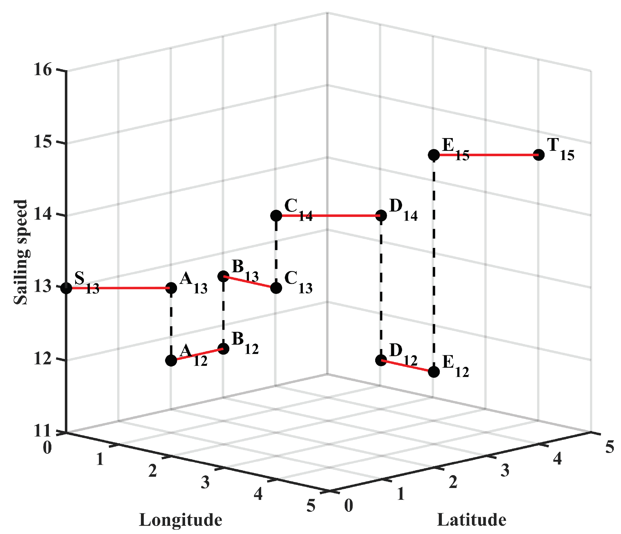
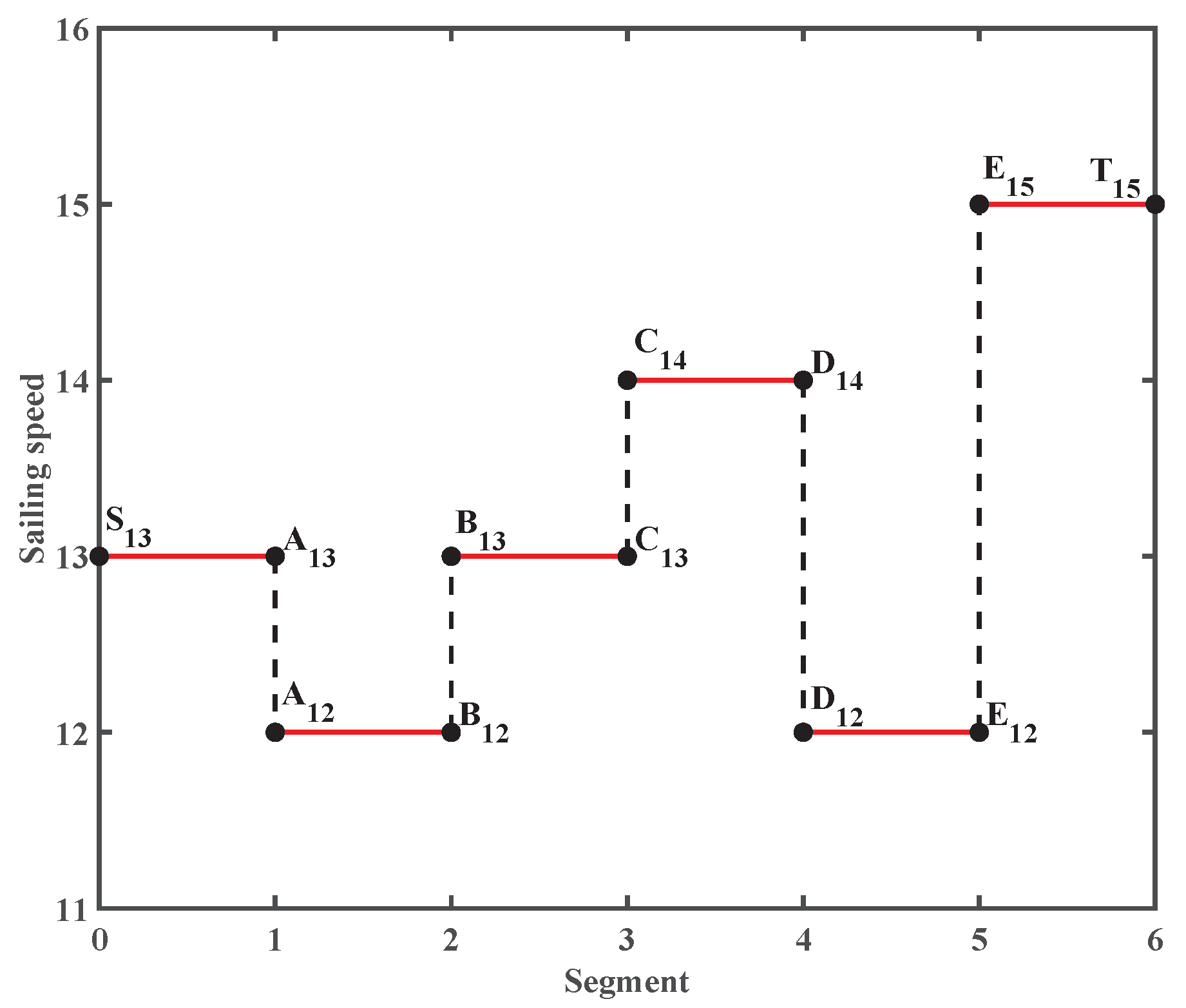
4.1. Speed Configuration
5. Weather Route Optimization for Ships with Sailing Time Constraints
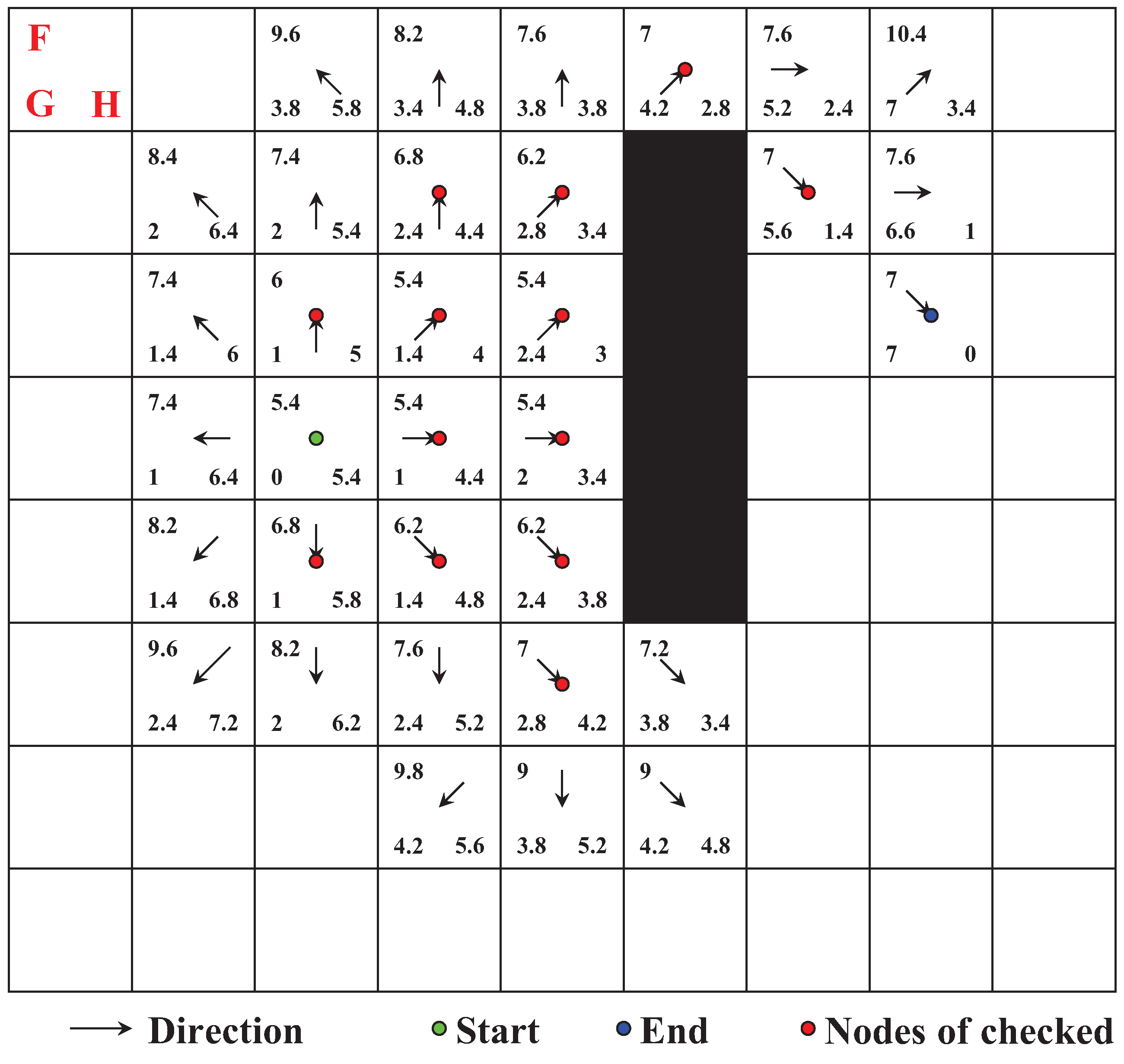
5.1. A* Algorithm
- The two-dimensional A* algorithm takes distance as the evaluation criterion. At the same time, ship fuel consumption and navigation time are the main factors to evaluate the navigation cost of a route, and taking distance as the evaluation criterion cannot accurately quantify the navigation cost.
- The two-dimensional A* algorithm does not consider speed. In contrast, the ship does not sail at a fixed speed over the whole voyage; dynamically adjusting speed according to the sea state is desirable.
- The two-dimensional A* algorithm does not consider dynamic unnavigable areas with heavy winds and waves, which will affect the safety and efficiency of the voyage.
5.2. Evaluation Functions Concerning Time and Fuel Consumption
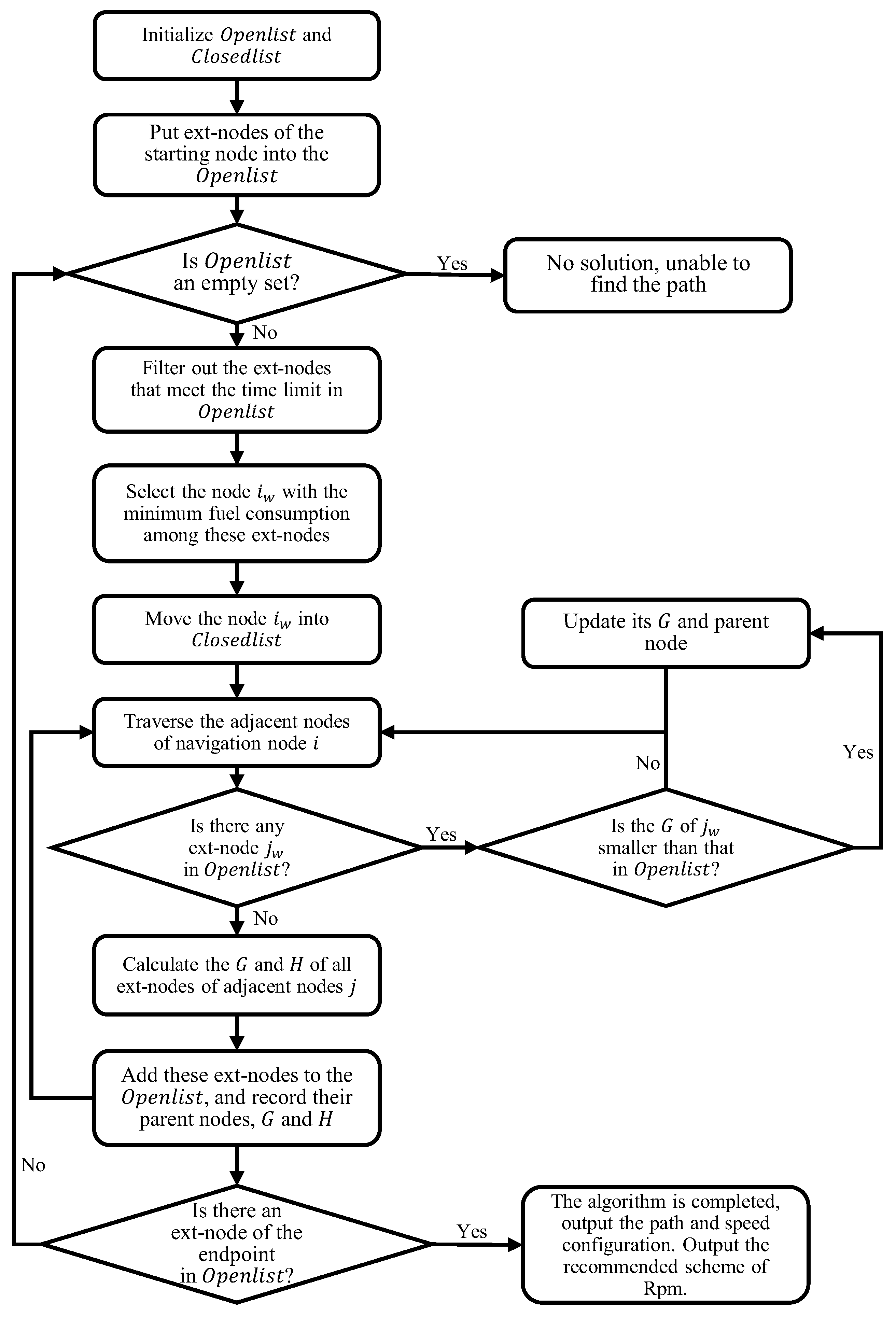
5.3. Customized A* Algorithm with Time Constraint
- Initialize (the set of ext-nodes to be checked) and (the set of ext-nodes checked).
- All ext-nodes belonging to the start node S are added to the , and their and are set to 0, while the and are calculated and recorded.
- If it is judged that the is not empty, the operation goes to Step 4; otherwise, there is no solution to this problem, which means no available path exists between S and T, and the procedure is terminated.
- The total navigation time of each ext-node in the is calculated. If the total navigation time of one ext-node is greater than the pre-set ETA, the node is retained in the but will not be executed in the rest of this step. Then, the ext-node with the minimum fuel consumption of the whole voyage is found in these nodes which meet the time limit. And the ext-node will be removed from the and added into the , setting the SOG record to .
- Traverse all the adjacent nodes of the navigation node i. There are two situations for the ext-nodes of these adjacent nodes:
- If there is no ext-node of the adjacent node j in and , all ext-nodes of node j are added to , the G and H value of these ext-nodes are calculated and recorded, and the parent node of these ext-nodes is set as node .
- If there is an ext-node of the adjacent node j in the , and the and values of calculated in this step are both smaller than those stored in the , the G and H values of in the will be updated correspondingly in this step. Also, the ext-node ’s parent node is set as node . Conversely, all information of the ext-node stored in will remain unchanged.
- Check whether there is any ext-node in that is subordinate to the end node T. If not, repeat Step 3; if it already exists, a path composed of ext-nodes is found by querying the parent node of the current ext-node step by step until the starting node. The sailing route and speed configuration are obtained after mapping like in Section 4.1.
- The weather forecast data and navigation data at each ext-node on the route are extracted based on the waypoint sequence and speed configuration. Then, the RPM prediction model is called, and the above data are modified as the input of the prediction model to calculate the recommended RPM of each ext-node on the route. Then, the RPM recommendation scheme is output for the whole voyage.
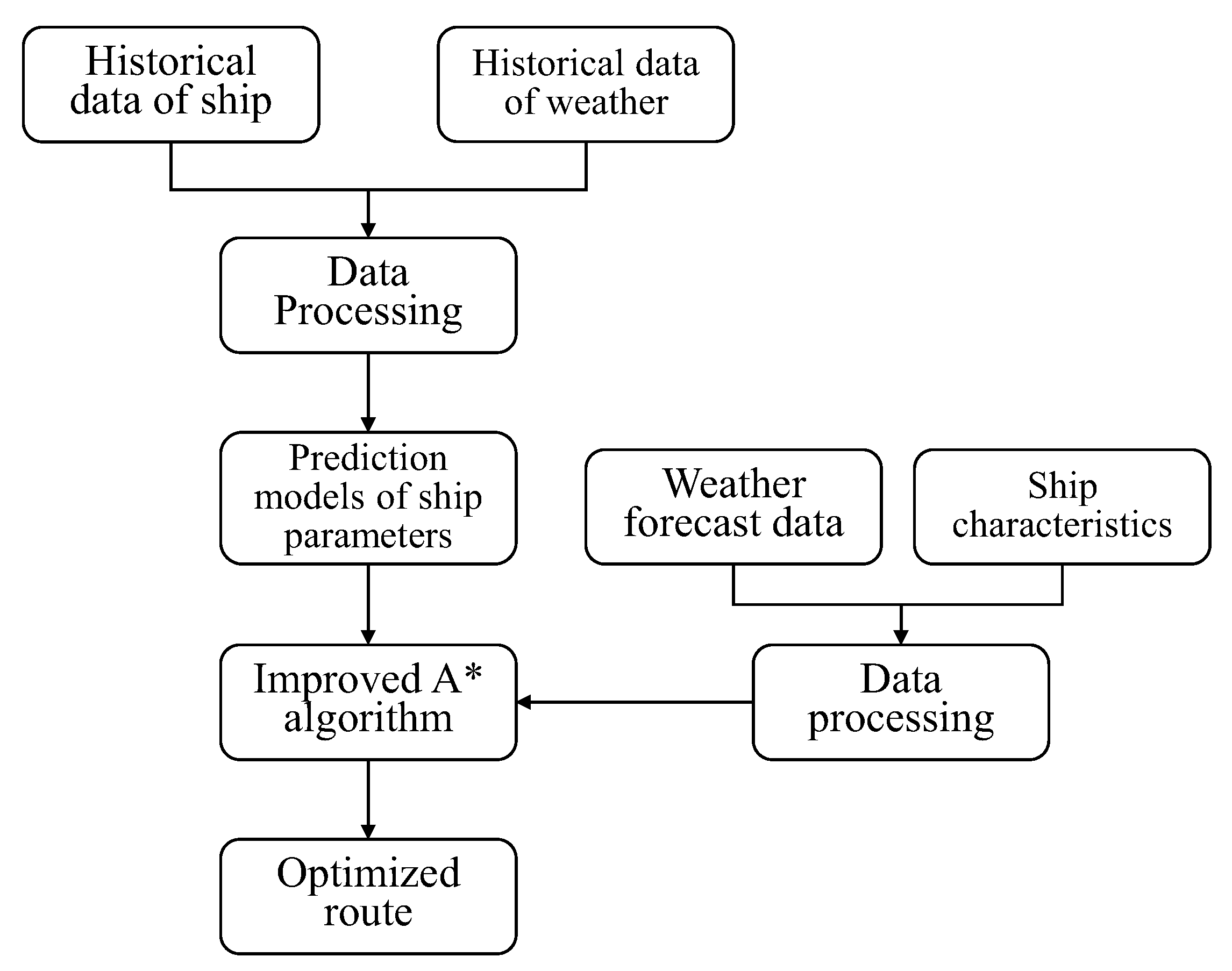
5.4. Overall Optimization Flow
- The historical data processing part uses historical ship voyage records and corresponding meteorological historical data, etc. These data are standardized by pre-processing data methods, and the pre-processed data are used as input for the ship parameter prediction models.
- The ship parameter prediction model part is used to build two artificial neural network models with the same frame. The input contains eight variables: SOG, fore draft, aft draft, course, wind speed, wind direction, wave height, and wave direction; the output is fuel consumption rate or RPM. The trained models are used for calculating fuel consumption rate and RPM in the voyage afterward.
- The ship navigation data processing part obtains and divides the ship’s characteristics and the weather forecast data into eight input variables which meet the requirements of the ship parameter prediction model and are used in the route planning process afterward.
- The ship route optimization part is based on the customized A* algorithm, using the ship fuel consumption rate prediction model and the current sailing data to calculate the fuel consumption for all nodes to be checked in order to find the node with the minimum fuel consumption that satisfies the ETA constraint and thus obtain the optimal ship route. Finally, the RPM recommendation scheme for the whole range is obtained based on the sailing data and the generated route.
6. Simulation Experiment and Results Analysis
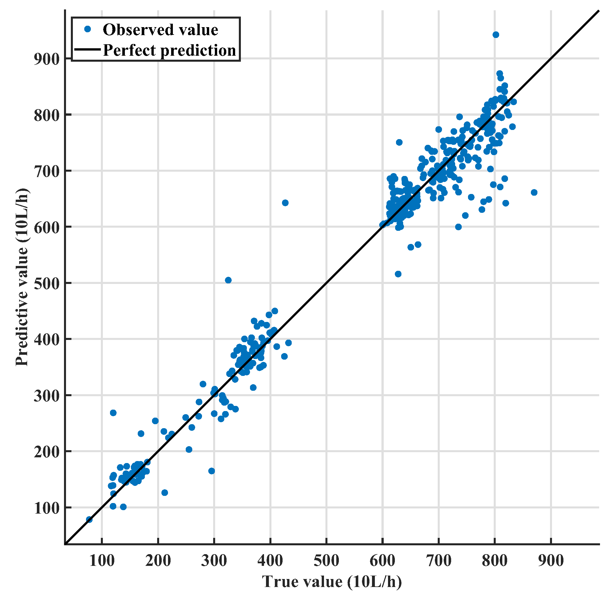
6.1. Performance Analysis of Ship Parameter Prediction Models
6.2. Simulation Experiment of Ship Weather Route Optimization System
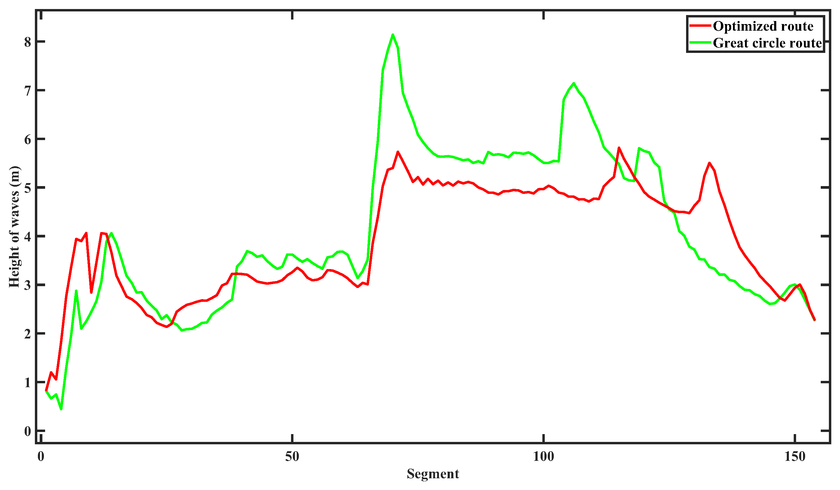
6.2.1. Scenario 1: Voyage from Osaka to Los Angeles on 3 February 2021
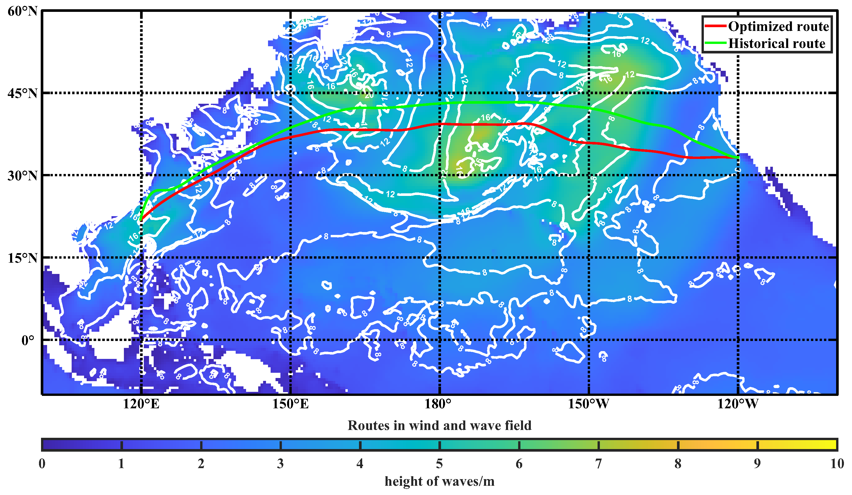
6.2.2. Scenario 2: Voyage from Tainan to Los Angeles on 17 January 2021
6.2.3. Computational Complexity of This Method
7. Conclusions
Author Contributions
Funding
Institutional Review Board Statement
Informed Consent Statement
Data Availability Statement
Conflicts of Interest
References
- Chircop, A. The IMO Initial Strategy for the Reduction of GHGs from International Shipping: A Commentary. Int. J. Mar. Coast. Law 2019, 34, 482–512. [Google Scholar] [CrossRef]
- Wang, H.; Mao, W.; Eriksson, L. Benchmark Study of Five Optimization Algorithms for Weather Routing. In International Conference on Offshore Mechanics and Arctic Engineering; American Society of Mechanical Engineers: New York, NY, USA, 2017; Volume 57748, p. V07BT06A023. [Google Scholar] [CrossRef]
- Simonsen, M.H.; Larsson, E.; Mao, W.; Ringsberg, J.W. State-of-the-Art within Ship Weather Routing. In Proceedings of the International Conference on Offshore Mechanics and Arctic Engineering. American Society of Mechanical Engineers Digital Collection, St John’s, NL, Canada, 31 May–5 June 2015. [Google Scholar] [CrossRef]
- Iphar, C.; Jousselme, A.L. A geometry-based fuzzy approach for long-term association of vessels to maritime routes. Ocean Eng. 2023, 281, 114755. [Google Scholar] [CrossRef]
- Pallotta, G.; Vespe, M.; Bryan, K. Vessel Pattern Knowledge Discovery from AIS Data: A Framework for Anomaly Detection and Route Prediction. Entropy 2013, 15, 2218–2245. [Google Scholar] [CrossRef]
- Wang, H.; Mao, W.; Eriksson, L. A Three-Dimensional Dijkstra’s Algorithm for Multi-Objective Ship Voyage Optimization. Ocean Eng. 2019, 186, 106131. [Google Scholar] [CrossRef]
- Hagiwara, H. Weather Routing of (Sail-Assisted) Motor Vessels. Ph.D. Thesis, Technical University of Delft, Delft, The Netherlands, 1989. [Google Scholar]
- Bijlsma, S.J. On Minimal-Time Ship Routing. Ph.D. Thesis, Delft University of Technology, Staatsdrukkerij Den Haag, The Netherlands, 1975. [Google Scholar]
- Bijlsma, S. On the Applications of Optimal Control Theory and Dynamic Programming in Ship Routing. Navigation 2002, 49, 71–80. [Google Scholar] [CrossRef]
- De Wit, C. Proposal for Low Cost Ocean Weather Routeing. J. Navig. 1990, 43, 428–439. [Google Scholar] [CrossRef]
- Padhy, C.P.; Sen, D.; Bhaskaran, P.K. Application of Wave Model for Weather Routing of Ships in the North Indian Ocean. Nat. Hazards 2008, 44, 373–385. [Google Scholar] [CrossRef]
- Liu, Y.; Wang, T.; Xu, H. PE-A* Algorithm for Ship Route Planning Based on Field Theory. IEEE Access 2022, 10, 36490–36504. [Google Scholar] [CrossRef]
- Wang, L.; Zhang, Z.; Zhu, Q.; Ma, S. Ship Route Planning Based on Double-Cycling Genetic Algorithm Considering Ship Maneuverability Constraint. IEEE Access 2020, 8, 190746–190759. [Google Scholar] [CrossRef]
- Pan, C.; Zhang, Z.; Sun, W.; Shi, J.; Wang, H. Development of Ship Weather Routing System with Higher Accuracy Using SPSS and an Improved Genetic Algorithm. J. Mar. Sci. Technol. 2021, 26, 1324–1339. [Google Scholar] [CrossRef]
- Zhao, W.; Wang, H.; Geng, J.; Hu, W.; Zhang, Z.; Zhang, G. Multi-Objective Weather Routing Algorithm for Ships Based on Hybrid Particle Swarm Optimization. J. Ocean Univ. China 2022, 21, 28–38. [Google Scholar] [CrossRef]
- Marie, S.; Courteille, E. Multi-Objective Optimization of Motor Vessel Route. TransNav Int. J. Mar. Navig. Saf. Sea Transp. 2009, 3, 133–141. [Google Scholar]
- Hinnenthal, J.; Clauss, G. Robust Pareto-optimum Routing of Ships Utilising Deterministic and Ensemble Weather Forecasts. Ships Offshore Struct. 2010, 5, 105–114. [Google Scholar] [CrossRef]
- Maki, A.; Akimoto, Y.; Nagata, Y.; Kobayashi, S.; Kobayashi, E.; Shiotani, S.; Ohsawa, T.; Umeda, N. A New Weather-Routing System That Accounts for Ship Stability Based on a Real-Coded Genetic Algorithm. J. Mar. Sci. Technol. 2011, 16, 311–322. [Google Scholar] [CrossRef]
- Lin, Y.H.; Fang, M.C.; Yeung, R.W. The Optimization of Ship Weather-Routing Algorithm Based on the Composite Influence of Multi-Dynamic Elements. Appl. Ocean Res. 2013, 43, 184–194. [Google Scholar] [CrossRef]
- Shao, W. Development of an Intelligent Tool for Energy Efficient and Low Environment Impact Shipping. Ph.D. Thesis, University of Strathclyde, Glasgow, Scotland, 2013. [Google Scholar]
- Skoglund, L.; Kuttenkeuler, J.; Rosén, A.; Ovegård, E. A Comparative Study of Deterministic and Ensemble Weather Forecasts for Weather Routing. J. Mar. Sci. Technol. 2015, 20, 429–441. [Google Scholar] [CrossRef]
- Zaccone, R.; Figari, M. Energy Efficient Ship Voyage Planning by 3d Dynamic Programming. J. Ocean Technol. 2017, 12, 49–71. [Google Scholar]
- Zaccone, R.; Ottaviani, E.; Figari, M.; Altosole, M. Ship Voyage Optimization for Safe and Energy-Efficient Navigation: A Dynamic Programming Approach. Ocean Eng. 2018, 153, 215–224. [Google Scholar] [CrossRef]
- Du, W.; Li, Y.; Zhang, G.; Wang, C.; Zhu, B.; Qiao, J. Energy Saving Method for Ship Weather Routing Optimization. Ocean Eng. 2022, 258, 111771. [Google Scholar] [CrossRef]
- Wen, Y.; Sui, Z.; Zhou, C.; Xiao, C.; Chen, Q.; Han, D.; Zhang, Y. Automatic Ship Route Design between Two Ports: A Data-Driven Method. Appl. Ocean Res. 2020, 96, 102049. [Google Scholar] [CrossRef]
- Vouros, G.A.; Vlachou, A.; Santipantakis, G.; Doulkeridis, C.; Pelekis, N.; Georgiou, H.; Theodoridis, Y.; Patroumpas, K.; Alevizos, E.; Artikis, A.; et al. Increasing Maritime Situation Awareness via Trajectory Detection, Enrichment and Recognition of Events. In Proceedings of the Web and Wireless Geographical Information Systems, A Coruna, Spain, 21–22 May 2018; R. Luaces, M., Karimipour, F., Eds.; Springer International Publishing: Cham, Switzerland, 2018. Lecture Notes in Computer Science. pp. 130–140. [Google Scholar] [CrossRef]
- Zis, T.P.; Psaraftis, H.N.; Ding, L. Ship Weather Routing: A Taxonomy and Survey. Ocean Eng. 2020, 213, 107697. [Google Scholar] [CrossRef]
- Du, Y.; Meng, Q.; Wang, S.; Kuang, H. Two-Phase Optimal Solutions for Ship Speed and Trim Optimization over a Voyage Using Voyage Report Data. Transp. Res. Part B Methodol. 2019, 122, 88–114. [Google Scholar] [CrossRef]
- Beşikçi, E.B.; Arslan, O.; Turan, O.; Ölçer, A.I. An Artificial Neural Network Based Decision Support System for Energy Efficient Ship Operations. Comput. Oper. Res. 2016, 66, 393–401. [Google Scholar] [CrossRef]
- Mao, W.; Rychlik, I.; Wallin, J.; Storhaug, G. Statistical Models for the Speed Prediction of a Container Ship. Ocean Eng. 2016, 126, 152–162. [Google Scholar] [CrossRef]
- Psaraftis, H.; Morales Llamas, J.; Ding, L.; Nehammer, J. BlueSIROS Project WP3, Proof of Concept; Technical Report, BlueSIROS Project Technical Report; Technical University of Denmark: Lyngby, Denmark, 2017. [Google Scholar]
- Newman, J.N. Marine Hydrodynamics; The MIT Press: Cambridge, MA, USA, 2018. [Google Scholar]
- Grifoll, M.; Martorell, L.; Castells, M.; de Osés, F.X.M. Ship weather routing using pathfinding algorithms: The case of Barcelona – Palma de Mallorca. Transp. Res. Procedia 2018, 33, 299–306. [Google Scholar] [CrossRef]
- Windeck, V. Environmental Routing. In A Liner Shipping Network Design: Routing and Scheduling Considering Environmental Influences; Windeck, V., Ed.; Produktion und Logistik, Springer Fachmedien: Wiesbaden, Germany, 2013; pp. 39–78. [Google Scholar] [CrossRef]
- Du, W.; Li, Y.; Zhang, G.; Wang, C.; Zhu, B.; Qiao, J. Ship weather routing optimization based on improved fractional order particle swarm optimization. Ocean Eng. 2022, 248, 110680. [Google Scholar] [CrossRef]
- Wang, H.; Lang, X.; Mao, W.; Zhang, D.; Storhaug, G. Effectiveness of 2D optimization algorithms considering voluntary speed reduction under uncertain metocean conditions. Ocean Eng. 2020, 200, 107063. [Google Scholar] [CrossRef]
- Hersbach, H.; Bell, B.; Berrisford, P.; Biavati, G.; Horányi, A.; Muñoz Sabater, J.; Nicolas, J.; Peubey, C.; Radu, R.; Rozum, I.; et al. ERA5 Hourly Data on Single Levels from 1940 to Present. Available online: https://cds.climate.copernicus.eu/cdsapp#!/dataset/reanalysis-era5-single-levels?tab=overview (accessed on 21 January 2022).
- GEBCO Compilation Group. GEBCO Gridded Bathymetry Data. Available online: https://www.gebco.net/data_and_products/gridded_bathymetry_data (accessed on 21 January 2022).
- Gkerekos, C.; Lazakis, I.; Theotokatos, G. Machine learning models for predicting ship main engine Fuel Oil Consumption: A comparative study. Ocean Eng. 2019, 188, 106282. [Google Scholar] [CrossRef]
- ISO 19030-2:2016; Ships and Marine Technology—Measurement of Changes in Hull and Propeller Performance — Part 2: Default Method. International Organization for Standardization: Geneva, Switzerland, 2016.
- Hu, Z.; Zhou, T.; Zhen, R.; Jin, Y.; Li, X.; Osman, M.T. A two-step strategy for fuel consumption prediction and optimization of ocean-going ships. Ocean Eng. 2022, 249, 110904. [Google Scholar] [CrossRef]
- Rumelhart, D.E.; Hinton, G.E.; Williams, R.J. Learning representations by back-propagating errors. Nature 1986, 323, 533–536. [Google Scholar] [CrossRef]
- Hagan, M.T.; Menhaj, M.B. Training Feedforward Networks with the Marquardt Algorithm. IEEE Trans. Neural Netw. 1994, 5, 989–993. [Google Scholar] [CrossRef] [PubMed]
- Hagan, M.T.; Demuth, H.B.; Beale, M.H. Neural Network ToolboxTM 6 User’s Guide; MathWorks: Natick, MA, USA, 2015. [Google Scholar]
- Shin, Y.W.; Abebe, M.; Noh, Y.; Lee, S.; Lee, I.; Kim, D.; Bae, J.; Kim, K.C. Near-Optimal Weather Routing by Using Improved A* Algorithm. Appl. Sci. 2020, 10, 6010. [Google Scholar] [CrossRef]









| Parameter | Value |
|---|---|
| Ship type | Container ship |
| Displacement (t) | 169,700 |
| Length (m) | 348 |
| Beam (m) | 51.2 |
| Draft (m) | 13.5 |
| Pitch (mm) | 8668 |
| Parameters | Value |
|---|---|
| Number of neurons in hidden layer of fuel consumption rate model | 45 |
| Number of neurons in hidden layer of RPM model | 140 |
| Activation function of the hidden layer | Relu |
| Optimizer | Levenberg–Marquardt |
| Parameters | Value |
|---|---|
| Start | 35.5 N, 141 E |
| End | 34 N, 120 W |
| SOG range (knot) | [8, 19] |
| Maximum allowable wind speed (m/s) | 20 |
| Maximum allowable wave height (m) | 6 |
| Minimum draught (m) | 14 |
| Time (h) | Danger Time (h) | |
|---|---|---|
| Optimized route | 367.15 | 0 |
| Great circle route | 361.38 | 26.26 |
| Time (h) | FOC (t) | |
|---|---|---|
| Optimized route | 408.69 | 1674.27 |
| Historical route | 404.34 | 1805.20 |
| Computational Time (s) | Data Size (MB) | |
|---|---|---|
| Scenario 1 | 991.917 | 1.10 |
| Scenario 2 | 731.639 | 1.04 |
Disclaimer/Publisher’s Note: The statements, opinions and data contained in all publications are solely those of the individual author(s) and contributor(s) and not of MDPI and/or the editor(s). MDPI and/or the editor(s) disclaim responsibility for any injury to people or property resulting from any ideas, methods, instructions or products referred to in the content. |
© 2023 by the authors. Licensee MDPI, Basel, Switzerland. This article is an open access article distributed under the terms and conditions of the Creative Commons Attribution (CC BY) license (https://creativecommons.org/licenses/by/4.0/).
Share and Cite
Li, Y.; Cui, J.; Zhang, X.; Yang, X. A Ship Route Planning Method under the Sailing Time Constraint. J. Mar. Sci. Eng. 2023, 11, 1242. https://doi.org/10.3390/jmse11061242
Li Y, Cui J, Zhang X, Yang X. A Ship Route Planning Method under the Sailing Time Constraint. Journal of Marine Science and Engineering. 2023; 11(6):1242. https://doi.org/10.3390/jmse11061242
Chicago/Turabian StyleLi, Yuankui, Jinlong Cui, Xinyu Zhang, and Xuefeng Yang. 2023. "A Ship Route Planning Method under the Sailing Time Constraint" Journal of Marine Science and Engineering 11, no. 6: 1242. https://doi.org/10.3390/jmse11061242
APA StyleLi, Y., Cui, J., Zhang, X., & Yang, X. (2023). A Ship Route Planning Method under the Sailing Time Constraint. Journal of Marine Science and Engineering, 11(6), 1242. https://doi.org/10.3390/jmse11061242


